An aerodynamic optimization design study on the bio-inspired airfoil with leading-edge tubercles

Abstract

The aim of the paper is to propose a groundbreaking method for the aerodynamic optimization design of the bioinspired wing with leading-edge tubercles. An emphasis on the optimization design of the spanwise waviness in the leading edge for delaying stall and increasing lift from the aerodynamic performance perspective has been laid in this study. For the conversion of the wavy configuration, the form parameterized approach using F-spline curves has been used to produce more variants of the leading-edge tubercles. Numerical investigations of flow characteristics which are performed using CFD computations have been used to validate the numerical scheme with experimental data. The combination of Non-dominated Sorting Genetic Algorithm II and Response Surface Method based Kriging Model has been adopted as the aerodynamic optimization strategy. As consequence, the three main components of the optimization process are incorporated into the establishment of the aerodynamic optimization design system for the bio-inspired airfoil with leading-edge tubercles. The four optimal airfoils respectively which increases the stall angle as well as the lift have been obtained in contrast to the smooth wing. The optimized bio-inspired design of this kind can be applied to flow-controlled devices for improving the efficiency of a particular operating mechanism.

KEYWORDS:

• Aerodynamic optimization
• bio-inspired design
• leading-edge tubercle
• lift
• angle of attack

1. Introduction

The successful bionic applications into mechanical systems have drawn numerous attention and inspiration from the researchers and engineers. Currently scientific and technological progress in various fields has made the dream of mimicking nature from a challenge to a reality (Choi, 2009; Fish, 2006; Fish et al., 2008). Because of its significant potential, explorations in the field of biomimetics have being obtained great popularity.

As a bionic representative, the humpback whale that belongs to the giant marine mammal possesses strong maneuverability which is propitious to predation in contrast to other marine mammals in analogous sizes. It can profit from several bulges on the leading edge of the humpback whale fins, which are made up of rounded protrusions (Favier et al., 2012; Fish et al., 2011; Shormann & Panhuis, 2019), varying from the smooth configuration. This special fin structure makes humpback whales perform tight turns such that they can catch prey limberly. Some experimental results show that the leading edge tubercles has some effect on improving the lift and stall characteristics, thus improving the aerodynamic performance of wing (Miklosovic et al., 2007; Stanway, 2008; Tunio et al., 2020; Weber et al., 2010). As is known, there are active and passive methods as the applications of flow control. Multiple technologies, including zero net mass flux (ZNMF) jets (Cater & Soria, 2002; Tuck & Soria, 2004), fluid injection (Seifert et al., 1993, 1996), trailing edge flaps (Borglund & Kuttenkeuler, 2002; Vipperman et al., 1998), and plasma generation (Post & Corke, 2004) at the wing surface are considered as the representatives of active methods. On the other hand, vortex generator (Mccormick, 1993), wing fences (Buchholz & Tso, 2000), leading edge extension (LEX) (Rao & Campbell, 1987), Gurney flaps (Wang et al., 2008), and leading edge modification (Fish & Battle, 1995) have been in used as the techniques applications of passive methods. The humpback flipper limbs can significantly improve underwater maneuverability of the whale, so the use of the leading edge tubercles projection to approximate the design has been suggested in some studies as a more passive approach to flow control.

In order to understand the concept of nodule, a lot of numerical calculations and experimental studies have been carried out (Corsini et al., 2013; Isaac & Swanson, 2011; Mehraban et al., 2020; Shi et al., 2016).

Previous studies on 3D wing leading edge nodules have reported different performance characteristics. These foils usually have tapered features such as rudders, stabilizers, wings, fins, etc. The influence of the hydrodynamic characteristics and the potential performance improvement brought about by the design of rudder wave-shaped leading edge has been examined and explored (Tae et al., 2017; Yoon et al., 2011). Moreover, studies have been conducted to define leading edge tubercles and serrated shapes on the airfoils and wings, showing improvements in their aerodynamic characteristics (Hansen et al., 2011; Johari et al., 2007).

The above researches clarified the influence of the geometry of humpback whale fin and waviness of the leading edge on flow. In addition, previous studies have focused on the standardization of the configuration of flipper, such as the regular trigonometric function curve configurations on the leading edge or rectangular wing, and the mechanical characteristics of the bionic-like wing. Meantime, it is difficult to discover some open-studies that handled with the real construction of the bio-airfoil and the arrangement of the tubercles on the humpback whale fins, and even the design of the wavy configurations from the perspective of practical bionic optimization. Therefore, the purpose of this study is to present a groundbreaking and effective method for the aerodynamic optimization of the bio-inspired airfoil with leading-edge tubercles. An optimal and real bionic airfoil which is of the property of high lift coefficient and large wing stall shall be obtained. To accomplish the optimization procedure, the transformation of airfoil, numerical computation and optimization strategy as the three main modules are established and integrated into the optimization design framework.

In terms of the airfoil model variation, it is the principal task throughout the aerodynamic wing optimization because this module determines the practicability and efficiency of the optimization process (Harries, 2007; Lee, 2003; Maisonneuve et al., 2003; Pérez & Clemente, 2011; Saha et al., 2004). To successfully obtain the deformation in control, there are four aspects which deserve consideration and contain design variables programmed, geometry alteration flexibility, fairing transition between the modified part and unchanged original part, as well as geometrical constraints. Though several popular modeling software which involves Catia and GMS/Facet as well as the NAPA have achieved certain progress in modeling, FRIENDSHIP-Framework which is believed to be the leading geometric modeling software package is provided with superiorities in the field of high degree of flexibility and convenience of variation. Under FRIENDSHIP-Framework software, the airfoil generation and transformation should be accomplished by controlling the F-spline curve, which can originate from the fair and optimized B-spline and curved surface (Abt et al., 2003; Mancuso, 2006), which could assure the automated design process effectively. In this study, it is the F-spline curve which is selected as the parameter representation for transformation of the leading-edge tubercles on airfoil. With respect to the second module in optimization system, that is numerical computation, it is of great significance to evaluate the aerodynamic performance accurately which is grounded on CFD. The usage of computational fluid dynamics as a necessary optimization step to investigate the flow characteristics around the airfoil has been carried out in a variety of studies, and it has been confirmed of reliableness and effectiveness (Dropkin et al., 2012; Watts & Fish, 2001). As for the optimization strategy, numerous related studies have handled with traditional optimization method which containing steepest descent method, conjugate gradient method and sequential quadratic programming method as well as response surface method (Kaymaz & McMahon, 2005; Peri et al., 2001; Ren & Chen, 2010; Valorani et al., 2003; Zhang et al., 2013) and some other intelligent optimization algorithms. The evolutionary algorithm (EA) and genetic algorithms (GAs) as well as particle swarm algorithms (PSO) and various improved algorithms (Grigoropoulos & Chalkias, 2010; Li et al., 2014; Liang et al., 2011) as example of the intelligent optimization algorithms have obtained the extensive applications and huge improvement in the number of soft computing technologies. Among these optimization techniques, the non-dominated sorting genetic algorithm II (NSGA-II) has been applied to solve the resolution of searching for optimal scheme (Jeyadevi et al., 2011; Srinivas & Deb, 1994). In this study, initially NSGA-II is used at initial optimization stage, then the response surface method based Kriging model has been adopted which is based on the initial optimization results from the NSGA-II computation. The practice of coupling optimization strategy would improve the optimization effectiveness on one hand and also totally expand the scope of search space, which can be revealed and explored in this study.

In the remainder of the article, the parametric transformation of the airfoil model with leading-edge tubercles by using an F-Spline parametric curve is proposed in Section 2. Then the numerical investigation based on CFD for the evaluation of flow characteristics is described in Section 3. In the next, the optimization strategy coupling the NSGA II and response surface method based Kriging model is explained in Section 4. After that, we have explored and circumstantiated the application of aerodynamic optimization design method with respect to bio-inspired wings in Section 5. At last, Section 6 puts forward the conclusions in terms of the proposed method.

2. Parametric transformation

2.1. Definition of the F-Spline parametric curve

Partial the theoretical approach to this content are given based on the following references (Birk & Harries, 2003; Harries, 1998). In the optimization design process, it is necessary to set up a series of parametric curves containing design variables in relation to the wing modification for ensuring the practicability and effectivity of the parametric modification of the airfoil. During the environment of the FRIENDSHIP-Framework, the F-Spline parametric curve is used, which is ground on the fairness-optimized B-Spline curve, with the shape parameter defined as a constraint. In common expression, the same parameter u is used to control the free curve vector r(u), which is the beginning positon of the vector: (1) $\mathit{r}(u)=(x(u),y(u),z(u))$(1)

In order for the mth order of the fairness criterion to be satisfied, the equation L_m relative to that is: (2) $L_m={\int }_0^1{(D^m\mathit{r}(u))}^2,\text{where }{D}^m=d^m/d{u}^m$(2)

This formula shall be subject to the following conditions:

Distance constraint: r(t)is obtained by the parameter knot t_i correlation, the Euclidean distance between a given data point P_i and r(t) is used, r(t) is given as a weighted definition, and finally in square form to limit the maximum positive error tolerance ϵ: (3) $A=\sum _{i=0}^n{[w_i(\mathit{r}(u_i)-P_i)]}^2\le \epsilon$(3)

Terminal constraint: the starting point and the endpoint of a curve given the value of i are 0 and n, respectively. Both endpoints are controlled by the vector Qi and the curvature vector Ki. The following equation is satisfied. (4) $T_1=D^1\mathit{r}(u_i)-{\mathit{Q}}_i=0$(4) (5) $T_2=D^2\mathit{r}(u_i)-{\mathit{K}}_i=0$(5)

Area constraint: the area under the curve is controlled by a given value S₀: (6) $F=S-S_0=0$(6)

Be aware that other types of equal or unequal forms of constraint must be taken into account as well. To complete the solution of the optimization problem with constraints, reconstructions of the combinations of the listed equations to the unconstrained function I: (7) $\begin{array}{rl}I& =L_m+\lambda A^{\mathrm{\prime }}+{\mu }_1{T}_1+{\mu }_2{T}_2+\nu F,\text{where}\\ & A^{\mathrm{\prime }}=A+d^2\end{array}$(7) where λ, μ₁, μ₂ and ν represent the Lagrange multipliers and d² represents a slack variable.

In the FRIENDSHIP-Framework runtime environment, the main attribute parameters of the F-Spline curve specifies: point coordinates (x, y, z) corresponding to tangent angle Qi and curvature Ki. area S and center coordinates (xC, yC, zC) of the sample curve, fairness E2. Therefore, such parametric curves optimized by finishing have great flexibility and high quality of shape, so that the F-Spline curve is applied as an intermediary to complete the corresponding smooth transformation of any part of the airfoil geometry.

2.2. Parametric curve based airfoil model transformation

Observing the humpback whale fins, there are different tubercles arranging on the leading edge. For completely modeling the bionic structure, this study employs exponential attenuation function as well as sinusoidal function for governing the arrangement and size of tubercles. In addition to this, adjusting the functions could give directions to the airfoil model transformation. The F-Spline curve is selected as the presentation of function curve which includes the amplitude and period as well as attenuation. The airfoil model may yield three types of transformation: the transverse amplitude translation of the tubercles, the longitudinal period translation of the tubercles and the longitudinal attenuation translation of the tubercles.

The airfoil model can produce three property transitions for tubercles: transverse amplitude, longitudinal period and longitudinal attenuation. In the present study, the F-Spline curve variation can be mapped to airfoil geometry transformation which is called the shifting method, accomplishing the parametric design process.

Take the longitudinal translation and transverse translation of the wing as examples, set δx_t as the maximum variable of the F-spline curve in the longitudinal X-axis direction and δy_t as the maximum variable of the curve in the transverse Y-axis direction. In either plane, both the F-spline curve and the airfoil will deform in either direction. In the XY plane, the transformation formula for the change of the point coordinates of the F-spline curve corresponding to the point coordinates on the geometric model is as follows: (8) $x_u=x+{\mathit{r}}_{\delta xu}(x)$(8) (9) $y_u=y+{\mathit{r}}_{\delta yu}(y)$(9) where r_δxt(x) and r_δyt(y) represent the update coordinates of the F-Spline curve connected to the input parameter δx_t, and x_t and y_t are the update point coordinates based on mapping the geometric position of the airfoil.

In order to avoid unreasonable turns and exaggerated changes in geometry, additional F-Spline curves in combination with transition curves. The curves are treated as weighted function curves for both longitudinal and transverse translations. It is assumed that δxw and δyw are changes in the end of the weighted function curve in both the longitudinal and transversal directions, usually 0<δx_w≤1 and 0<δy_w≤1. Based on the given original coordinates and the weighted function, a controlled update of the coordinate points is obtained, which is rewritten as follows: (10) $x_u=x+{\mathit{r}}_{\delta xu}(x)\cdot {\mathit{r}}_{\delta xw}(x)$(10) (11) $z_u=z+{\mathit{r}}_{\delta zu}(z)\cdot {\mathit{r}}_{\delta zw}(z)$(11) where r_δxw(x) and r_δyw(y) are given as weight function curve coordinates for the input parameters δ_xw, i.e. the positions of mapping wing model.

The bio-inspired airfoil with leading-edge tubercles used in this paper is based on a smooth airfoil in which the model comparisons are illustrated in Figure 1. The bionic airfoil model shall be fully parameterized with the help of the transformation rules proposed above in order to develop large number of shapes with respect to diverse aerodynamic characteristics. Based on the F-Spline curve variation, these three types of airfoil transformations are shown in Figures 2–4.

Figure 1. Comparison of the geometries for the two airfoils: (a) The smooth airfoil; (b) The wavy airfoil.

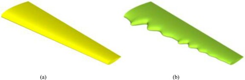
Figure 2. Comparison of the transverse amplitude translation of the leading-edge tubercles: (a) Transverse low amplitude translation; (b) Transverse large amplitude translation.

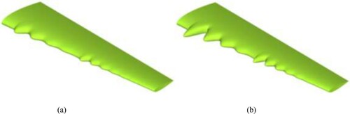
Figure 3. Comparison of the longitudinal period translation of the leading-edge tubercles: (a) Longitudinal long-period translation; (b) Longitudinal short-period translation.

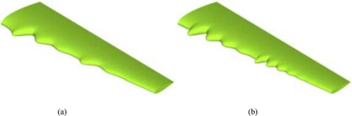
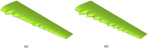
Figure 4. Comparison of the longitudinal attenuation translation of the leading-edge tubercles: (a) Longitudinal rapid attenuation translation; (b) Longitudinal slow attenuation translation.

3. Numerical investigations

3.1. Governing equations

In this section, the CFD-based numerical method is referenced in Ref (Akbarian et al., 2018; Ramezanizadeh et al., 2019; Salih et al., 2019) for the application to the flow simulation and the evaluation of aerodynamic performance has been described. The computational fluid dynamics STAR CCM+ is adopted throughout the numerical simulations. In this paper, the three-dimensional problem is considered by solving the Reynolds-averaged Navier-Stokes equation. The equation is defined as non-constant, incompressible and viscous flow. The governing equations can be written as: (12) $\begin{array}{rl}& \frac{\mathrm{\partial }(\rho u_i)}{\mathrm{\partial }{x}_i}=0\end{array}$(12) (13) $\begin{array}{rl}& \frac{\mathrm{\partial }(\rho u_i)}{\mathrm{\partial }t}+\frac{\mathrm{\partial }(\rho u_i{u}_j)}{\mathrm{\partial }{x}_j}\\ & =-\frac{\mathrm{\partial }p}{\mathrm{\partial }{x}_i}+\frac{\mathrm{\partial }}{\mathrm{\partial }{x}_j}\left[\mu \left(\frac{\mathrm{\partial }{u}_i}{\mathrm{\partial }{x}_j}+\frac{\mathrm{\partial }{u}_j}{\mathrm{\partial }{x}_i}\right)\right]+\frac{\mathrm{\partial }}{\mathrm{\partial }{x}_j}(\rho \overline{{u_i}^{\mathrm{\prime }}{u_j}^{\mathrm{\prime }}})\end{array}$(13) where u_i, p, t, ρ, μ, and $\rho \overline{{u_i}^{\mathrm{\prime }}{u_j}^{\mathrm{\prime }}}$ are the velocity, pressure, time, density, viscosity coefficient, and Reynolds stress, respectively.

3.2. Numerical method

In this study, the SIMPLE algorithm in a QUICK spatial discretization format supported by a finite volume approach is utilized to solve the control equations. Since the flow is in transition range in the present study, we have adopted γ-Reθ co-relation model. The γ-Reθ co-relation model (Langtry, 2006; Menter et al., 2004) is a two-equation, a semi-local method based on a correlation-based transition model is provided to predict the occurrence of transitions in the turbulent boundary layer. The transition model refers to a correlation-based transition model that is specific to unstructured CFD codes. By relating this quantity to a vorticity-based Reynolds number the evaluation of momentum thickness Reynolds number is avoided.

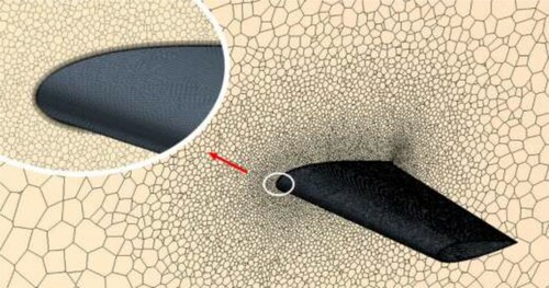
In Figure 5, the computational domain, boundary condition settings, and coordinate axis system of this computational work are shown. Using a fixed Cartesian coordinate system (x, y, z), the origin is at the terminal of the root. The x-axis is parallel to the direction of the inlet airflow and oriented towards the outlet. z-axis is parallel to the wing span and oriented from the pressure surface to the suction surface, and y-axis is perpendicular to the x-axis and z-axis and oriented from the tip to the root. The computational domain size in the x-direction, vertical z-direction and spreading y-direction is 4, 2 and 0.35 m, respectively. When it comes to the boundary conditions, the velocity inlet is uniformly flowing (U_∞) at the incoming boundary conditions. The outflow boundary is set with a pressure exit condition. Apply a no-slip boundary condition on the wing, upper and lower boundaries. Symmetrical boundary conditions are set at the two boundaries in the x-y plane. The grid system near the wavy airfoil shown in Figure 6. The minimum grid spacing on the surface of the wing averaged over the wall distance y+ corresponds to less than 1. The grid of the computational domain excluding the grid on the surface of the wing is continuously thickening with increasing distance from the wing, which could be automatically generated with the use of the macro file that are compiled and run under the CFD environment.

Figure 5. Computational domain, boundary condition settings, and coordinate axis system of this computational work.

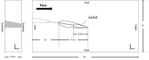
Figure 6. Meshing near the surface of the airfoil.

3.3. Validation of numerical scheme

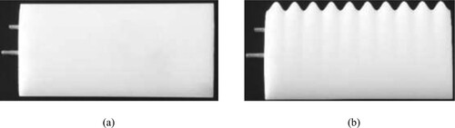
For the aim of verifying the numerical methodology proposed, we have performed the air flow simulations in accordance with the Ref (Yasuda et al., 2019) experimental conditions of the smooth wing whose cross-sectional profile is a smooth wing of NACA0012 with a chord ratio of 2. The chord length is defined as c = 0.055 m and the span length as 0.11 m. In addition the other experimental airfoil is equipped with a sinusoidal leading edge protuberance with an amplitude of 0.05c and a wavelength of 0.2c, and with the angles of attack (α) at 4 and 14 degree, Re = 0.432×10⁵. In Figure 7, the two airfoil models used in the experiment being in consistent with the numerical simulation have been shown.

Figure 7. Airfoil models in the experiment (Yasuda et al., 2019): (a) The smooth airfoil; (b) The airfoil with sinusoidal leading edge protuberance.

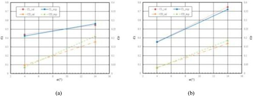
By comparing this study the calculation results of lift coefficient (C_L), and drag coefficient (C_D) and the Ref (Yasuda et al., 2019) the result of the experiment, found that are in good agreement, as shown in Figure 8. Although there are some differences in the numerical values of the force coefficients calculated by comparing previous studies. It can be considered that this is due to the inherent three-dimensional instability in the flow. The vortex structure caused by three-dimensional leading edge separation may be relatively complex. It is also discovered especially for the simulation of the leading edge protuberance wing that the comparison difference has decreased gradually.

Figure 8. C_L and C_D results between numerical simulation and experiment data for: (a) The smooth airfoil; (b) The airfoil with sinusoidal leading edge protuberance.

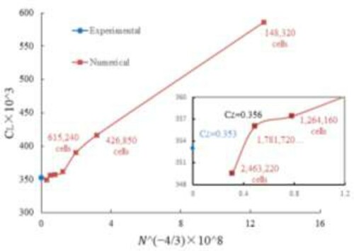
In order to eliminate the effect of grid resolution on the accuracy of the simulation, the convergence of lift coefficient and the number of grid cells was verified, the smooth wing of grid system at Re = 0.432×10⁵ and the angles of attack (α) ranging at 4 degree is shown in Figure 9. As a result, it is found that 1,781,720 grid units are enough to reach the convergence of lift coefficients in all grid number scales and the error in C_L is 0.85% for the finest grid.

Figure 9. The lift coefficient plotted against the grid factor (N^−4/3) (shown in the subplot with the black dashed line) for the three finest numerical meshes.

4. Optimization strategy

4.1. Non-dominated sorting genetic algorithm II

The optimization algorithm is of great significance for the airfoil deformation optimization by providing optimized design variables and guiding optimal search direction. In this study, the Non-Dominance Sorting Genetic Optimization Algorithm (NSGA-II) is used as a first step to the overall strategy of optimize. It is inspired by the fact that genetic algorithms (GAs) simulate biological evolution, which is a set of phenomena such as natural selection and genetic manipulation. Subsequently, in order to reduce the computational complexity O(mN³) to a maximum of O(mN²) calculations, NSGA-II (Deb et al., 2000) was proposed as an important improvement based on the fast non-dominant ranking method.

In the fast non-dominant sorting method, two parameter attributes of n_i and S_j are first assigned to each dominant individual in the population. An existing set F₁ is established to set the individuals, and all individuals in the set n_i=0 are sorted into the current set F₁. Then the set of S_j individuals is checked, and the dominant number n_k is set for each set S_j-1, that is, the number of individuals dominating k - 1 individuals. If n_k-1 = 0, then individual j is adjusted and stored in another group H. Finally, the set of F₁ first-level non-dominated individuals is set for the same non-dominated i_rank individual. Continue the sorting operation H above, and assign the corresponding non-dominated order until the individuals are ordered. For the purposes of population diversity in the optimization calculation, the evaluation and comparison of the crowding degree is employed, It is conducted by using i_d to represent the density of any individual i, and representing the smallest rectangle containing only the individual itself. When the value of i_d is small, it means that the individual is crowded around. Each individual i in the group is given a non-dominant order i_rank and a congestion i_d by computing the two properties ordering and congestion, then the partial order relationship is defined as ${\prec }_{\text{n}}$: when demand i_rank < j_rank or i_rank = j_rank is satisfied, When i_d > j_d, define $\text{i}{\prec }_{\text{n}}\text{j}$. 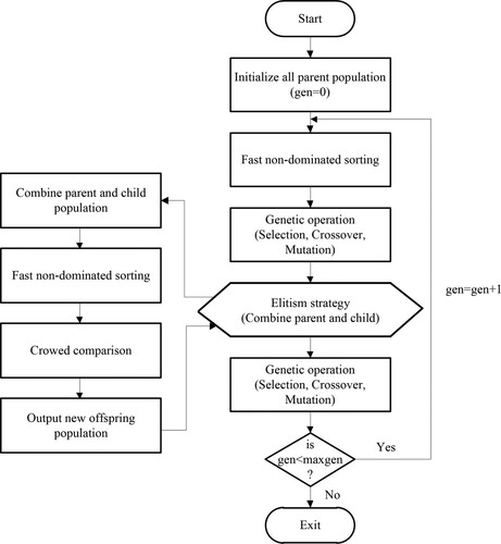It has been indicated that if the non-dominated order of two individuals is different, take the individual with the smaller order number. In the case of two individuals belonging to the same level, the less crowded individual around them is taken. The elite strategy is introduced in the NSGA-II algorithm by merging and combining every two adjacent generations, and fast non-dominated sorting, crowding degree evaluation and comparison are adopted, finally obtaining a new generation of excellent population to complete the genetics and other operations. Based on the above expressions, the flowchart of the NSGA-II algorithm is shown in Figure 10.

Figure 10. The flowchart of the NSGA-II algorithm.

4.2. Response surface method based Kriging model

When faced with large optimization problems based on numerical simulations that would take a long time, sampling traditional design tools and optimization algorithms is difficult for designers to accept. The response surface method is an effective way to solve such problems. As one of the proxy models of the response surface method, Kriging is a high-precision interpolation response surface model (Sakata et al., 2004) that expresses the functional relationship between design variables and response variables by using the sum of a regression function and a random process. In the process of optimization, the Kriging model is used to analyze the search of the relationship between the design variables and the objective function. Kriging behavior is controlled by the covariance function in which this rule determines how to change the correlation between function values at different points. It can show a larger or smaller range of variation, accept a certain amount of error, and all of these functions can be restored in the variance plot model. The information such as valuation and variance can effectively guide the optimization search toward the global direction. The following describes the standard Kriging model:

Let x₁, … , x_n be a given series of design points, and z(x₁), … , z(x_n) be corresponding response values. The value z*(x) of the range variable at x can be estimated using a linear combination: (14) $z^{\ast }(x)=\sum _{i=1}^n{\lambda }_{i}z(x_i)$(14) Among them, the fitting quantity λ_i is the position weight at the measured value at the i-th point, which needs to satisfy the two conditions of unbiased condition and minimum variance estimation. Meanwhile z*(x) is the predicted value at point x, n is the number of actual measured values, z*(x_i) is the actual measured value at the i-th point.

An unbiased condition is a mathematical expectation that the deviation of the true value from the estimated value is zero. The ordinary Kriging equation is established under the assumption that the Eigen conditions are satisfied, that is, the mathematical expectation of the regionalized variable z(x) is an unknown constant, namely: (15) $E[z(x)]=m$(15)

To ensure that z*(x) is an unbiased estimate of z(x), that is: (16) $E[z^{\ast }(x)-z(x)]=0$(16)

Given the Equation (15), the above formula can be reduced to: (17) $\begin{array}{rl}E[z^{\ast }(x)-z(x)]& =E\left[\sum _{i=1}^n{\lambda }_{i}z(x_i)-z(x)\right]\\ & =\left(\sum _{i=1}^n{\lambda }_i\right)m-m=0\end{array}$(17) So we can get ${\sum }_{i=1}^n{\lambda }_i=1$, which is the unbiased condition of ordinary kriging.

The optimality condition is that under the premise of satisfying the unbiased condition, the estimated variance shall be the smallest, that is: (18) $Var[z(x)-z^{\ast }(x)]=min$(18)

It can be transformed into: (19) $\begin{array}{rl}{\delta }_k^2& =E[\{(z^{\ast }(x)-z(x))-E(z^{\ast }(x)-z(x)){\}}^2]\\ & =E[(z^{\ast }(x)-z(x){)}^2]=min\end{array}$(19)

Applying the Lagrange multiplier method to find the conditional extreme value, then the n + 1 order linear equations can be derived, that is, the kriging equations: (20) $\left\{\begin{array}{l}\sum _{i=1}^{n}C(x_i-x_j){\lambda }_i-\mu =C(x-x_j)\stackrel{}{}\stackrel{}{}(j=1,\dots ,n)\\ \stackrel{}{}\stackrel{}{}\stackrel{}{}\stackrel{}{}\stackrel{}{}\stackrel{}{}\stackrel{}{}\stackrel{}{}\stackrel{}{}\sum _{i=1}^n{\lambda }_i=1\end{array}\right\}$(20)

When the random function does not satisfy the second-order stationary assumption, but meets the Eigen assumption, the kriging equations can be represented by the variation function: (21) $\left\{\begin{array}{l}\sum _{i=1}^n\gamma (x_i-x_j){\lambda }_i-\mu =\gamma (x-x_j)\stackrel{}{}\stackrel{}{}(j=1,\dots ,n)\\ \stackrel{}{}\stackrel{}{}\stackrel{}{}\stackrel{}{}\stackrel{}{}\stackrel{}{}\stackrel{}{}\stackrel{}{}\stackrel{}{}\sum _{i=1}^n{\lambda }_i=1\end{array}\right\}$(21)

In virtue of the response surface method based Kriging incremental model, an efficient global approximation optimization can be realized. The implementation and application of incremental construction can greatly improve the modeling efficiency and ensure the accuracy and stability of the global approximate model. Especially for the condition of adopting single intelligent optimization algorithms, such as the Gas as well as the NSGA II and so on, this practice is provided with low computation efficiency and high time consuming for the viscous flow calculation by CFD to some degree though possessing powerful ability of global searching. Therefore the present study has employed the Kriging method which uses efficient calculation speed to provide a smooth, global approximate function relationship for the source model which can be offered by initial NSGA II optimization, completing full optimization in further step.

5. Aerodynamic optimization of bio-inspired airfoil

5.1. Airfoil model with leading-edge tubercles description

In this study, the two geometries for the aerodynamic performance comparison which are the bio-inspired airfoil with leading-edge tubercles and a smooth airfoil keep the same chord length of the root (C_root = 0.1 m) and chord length of the tip (C_tip = 0.05 m) as well as the span (S = 0.35 m), so with the same AR. The difference falling in the bio-inspired airfoil is the generation of leading-edge tubercles which is the key point for the aerodynamic optimization design by the tubercles shape transformation. Under the condition of Reynolds number (Re = U_∞Cρ/μ) 10⁵, the flow around three-dimensional airfoil with naca0020 as the section is calculated for the range of multiple attack angles.

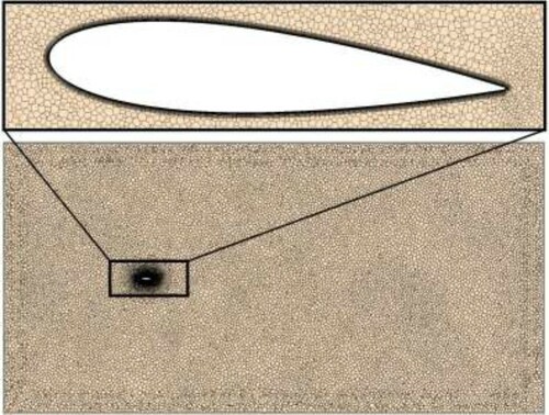
For ensuring the calculation accuracy, the volume mesh around the airfoil has been refined either for the smooth model or the wavy configuration which keep the same settings with that of the previous smooth wing with the section profile of NACA0012 or the sinusoidal leading edge protuberance airfoil in the subsection 3.3 of validation of numerical scheme. Also, the block surrounding mesh of the airfoil has been densified additively which are depicted in Figure 11, resulting in the total mesh number of 2.67 million.

Figure 11. Computational grid of the airfoil.

5.2. Optimization set-up

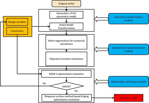
With the combinations of the flexible model parametric transformation, the reliable aerodynamic performance CFD prediction technology and the robust optimization algorithms, the optimization design framework of the bio-inspired airfoil with leading-edge tubercles would be analyzed and established. Firstly, with the input of design variables, a bio-inspired airfoil geometry file is generated using the parametric transformation technology module. Then, the transformed model information would flow into the airfoil aerodynamic performance prediction module where the calculation mesh will complete regeneration and the objective functions could output. Next, the NSGA II optimization algorithm shall adjust the search for new design variables by considering the aerodynamic results and constraints. Repeats the above implementation, the initial optimal scheme will be obtained. In the last place, ground on the information on all of the NSGA II optimization individuals, the response surface method based Kriging model will be employed for further global searching, obtaining the final optimal airfoil. Using the python programming language and the required network protocols, the three main modules enable communication and data exchange between the optimized systems. The optimization of the aerodynamic design framework integration process is shown in Figure 12.

Figure 12. The flow chart of the bio-inspired airfoil optimization design system.

Throughout the optimization design process, the stall angle and the lift coefficient of airfoil at stall as the typical criterions for the evaluation of aerodynamic performance has been defined to be the objective functions. Therefore the present study is concentrated on the multi-objective optimization issue. In terms of design variables which could develop different wavy configurations, the leading-edge tubercles of the bio-inspired airfoil yields the distortion transformation as illustrated in subsection 2.2. The specific definition of the design variables are: $A_1,A_2,T_1,T_2,E_1,E_2$where A₁ and A₂ control the transverse amplitude translation of the leading-edge tubercles, T₁ and T₂ handle with the longitudinal period translation of the leading-edge tubercles, E₁ and E₂ could modify the longitudinal attenuation translation of the leading-edge tubercles. These design variables shall generate the tubercles into different structures with respect to sizes, numbers and arrangement. Moreover, according to the design variables introduced above, the constraints for specific deformation control in conjunction with the design variables are as follows: $\begin{array}{l}0.5\le A_1\le 1.0,{}^{}2.0\le T_1\le 6.0,{}^{}0.5\le E_1\le 3.0,\\ 1.0\le A_2\le 1.5,{}^{}2.0\le T_2\le 6.0,{}^{}0.5\le E_2\le 3.0\end{array}$where A₁ and A₂, T₁ and T₂, E₁ and E₂ are the nondimensional parameters, respectively.

5.3. Results and discussion

During the optimization process, the NSGA-II is firstly adopted in which set the population of each generation to 10 and the generation number to 12 to find the initial optimal airfoil form under all necessary constraints. In a further step, we have adopted the response surface method based Kriging model by using the initial optimization results, as a consequence the number of the global searching is about 9000 individuals. During the investigation on the optimization design, the solution set of the objective functions including the stall angle α (F₁) and the lift coefficient C_L (F₂) has been shown in Figure 13.

Figure 13. The solution set of objective functions F1 and F2 of optimization.

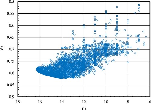
Figure 14. Lift coefficient under different angles of attack for optimal airfoils and the smooth airfoil.

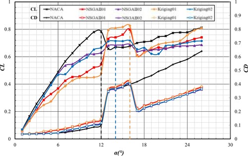
It can be discovered from the Figure 13 that the two objective functions have formed the Pareto front shape. Based on the Pareto solution set, we have selected two optimal schemes from the result of response surface method based Kriging model and two optimal schemes from the NSGA-II optimization. In addition, the lift coefficients of the four optimal airfoils (Name: NSGAII01, NSGAII02, Kriging01, Kriging02) and the smooth airfoil (Name: NACA) as according to the angle of attack have been depicted in Figure 14.

As can be seen in Figure 14, the stall angle for the airfoils ranging from the smooth airfoil (Name: NACA) and four optimal airfoils (Name: NSGAII01, NSGAII02, Kriging01, Kriging02) are 12, 16, 16, 16, 14 deg, respectively. From the Figure 13, it can be illustrated that the Kriging01 airfoil possess high lift coefficient and stall at the angle of attack 16 deg among the four optimal schemes but it is much better than that of the NACA wing. At the same time, the NSGAII02 airfoil has batter drag performance though its stall angle is the least. Figures 15–17 show the distribution of pressure coefficients (C_P) on the upper and lower surface of smooth airfoils, as well as the four optimal airfoils with wide range of the airfoil attack angles.

Figure 15. C_P on the upper surface (up) and the lower surface (low) at α=4 deg for different airfoils: (a) NACA; (b) NSGAII01; (c) NSGAII02; (d) Kriging01; (e) Kriging02.

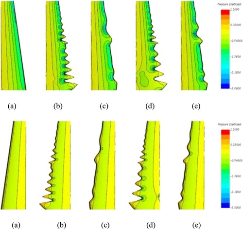
Figure 16. C_P on the upper surface (up) and the lower surface (low) at α=8 deg for different airfoils: (a) NACA; (b) NSGAII01; (c) NSGAII02; (d) Kriging01; (e) Kriging02.

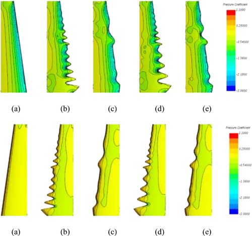
Figure 17. C_P on the upper surface (up) and the lower surface (low) at respective stall angle for different airfoils: (a) NACA; (b) NSGAII01; (c) NSGAII02; (d) Kriging01; (e) Kriging02.

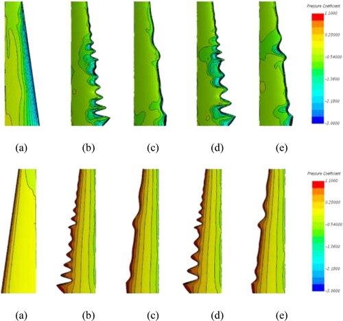
For the NACA airfoil, it can be seen from the above results of Figures15(a)–17(a) that at the angle of attack α=4° the C_P on the upper surface gradually decreases in the region beginning with the trailing edge to the leading edge. As closing to the leading edge, the pressure coefficient increases slightly, appearing negative pressure zone. On the contrary, the pressure coefficient of the lower surface is growing down by degrees beginning with the trailing edge to the leading edge. With the increase of the attack angle up to stall, the variation of the distribution of C_P for the upper surface as well as the lower surface are basically the same as those at α=4°.

Regarding to the four optimal airfoils, it can also be observed from Figures15(b–e)–17 (b–e) that under the condition of α=4°, though the C_P on the upper surface declines beginning with the trailing edge to the leading edge but it increases near the leading edge. A negative pressure area arises at the trough of the leading-edge tubercles, along the lengthening direction. In addition, the pressure coefficient at the crest of the concave and convex nodules has diminished little by little along the spanwise. Inversely on the lower surface of the airfoils, the pressure coefficient reduces beginning with the trailing edge to the leading edge. As the angle of attack rising till the respective stall angle for each optimal airfoil, the variation tendency of pressure coefficient distribution on both wing surfaces keep accordance with the condition of α=4°, the difference fall in the values of C_P.

It is worth noting that at α=4°, the C_P on the lower surface of NACA airfoil is more uniform than that of four optimal airfoils, as a result the lift coefficient at this angle of attack is greater than that of the concave–convex airfoils. With the angle of attack growing, since the NACA airfoil come about stalling with sharp decrease of lift coefficient after the attack angle of 12°. But the lift coefficients of the bio-inspired airfoils continue to increase before stalling, where the pressure coefficient distribution of the bio-inspired airfoils gradually seems uniform. This is consistent with the results presented in Figure 14. Meanwhile the skin friction coefficient (C_F) on the upper surface of the smooth airfoil and the four optimal airfoils in a wide range of attack angles α has been presented in Figures 18–20.

Figure 18. C_F on the upper surface (up) at α=4 deg for different airfoils: (a) NACA; (b) NSGAII01; (c) NSGAII02; (d) Kriging01; (e) Kriging02.

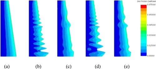
Figure 19. C_F on the upper surface (up) at α=8 deg for different airfoils: (a) NACA; (b) NSGAII01; (c) NSGAII02; (d) Kriging01; (e) Kriging02.

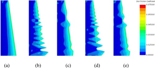
Figure 20. C_F on the upper surface (up) at respective stall angle for different airfoils: (a) NACA; (b) NSGAII01; (c) NSGAII02; (d) Kriging01; (e) Kriging02.

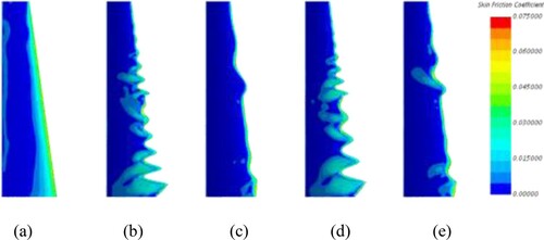
From Figures 18–20, it can be observed on the upper surface that the zero-free region of the surface friction coefficient of each airfoil gradually decreases as the angle of attack increases. While the attack angle reaches 12 deg that is its stall angle, the skin friction coefficient of zero-free region for the NACA airfoil mostly covers the whole upper surface. Until the angle of attack goes up to the respective stall angle (16, 16, 16 deg and 14deg) for each optimal airfoil, the skin friction coefficient of zero-free region has just hooded the upper surface basically but the larger the coefficient of surface friction with the closer to the leading edge. In contrast, axial velocity profiles of four sections at the stall condition that are considered for each airfoil have been plotted in Figures 21–25.

Figure 21. Axial velocity profile on different sections positions with the length ratio (10%, 25%, 50%, and 75%) of the span for NACA airfoil at the stall angle 12°.

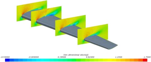
Figure 22. Axial velocity profile on different sections positions (the first crest, the second trough, middle, and the last trough) of the leading-edge for NSGAII01 airfoil at the stall angle 16°.

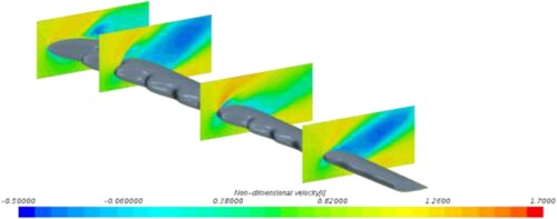
Figure 23. Axial velocity profile on different sections positions (the first crest, the second trough, middle, and the last trough) of the leading-edge for NSGAII02 airfoil at the stall angle16°.

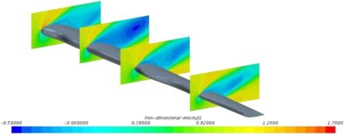
Figure 24. Axial velocity profile on different sections positions (the first crest, the second trough, middle, and the last trough) of the leading-edge for Kriging01 airfoil at the stall angle 16°.

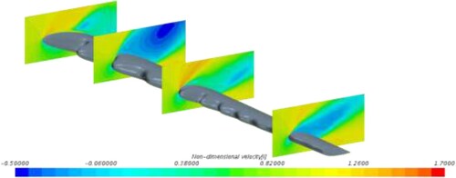
Figure 25. Axial velocity profile on different sections positions (the first crest, the second trough, middle, and the last trough) of the leading-edge for Kriging02 airfoil at the stall angle 14°.

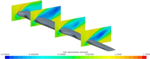
As shown in Figures 21–25, we can discover that the length ratio 10% of the span, it is determined by average positions of each fa marked difference in the axial velocity contours occurs between the sections taken at crest and trough for the optimal airfoils. In terms of selection of the planes for NACA airfoil, such as the first section with tirst crest of these bio-inspired airfoils, so with the same practice with other sections. Along the spanwise, the axial velocity magnitude of each airfoil on the four sections has been decrescent and the negative velocities zone becomes larger. With respect to the first section, higher positive velocities occur for NACA airfoil than that of four airfoils where it is located at the first crest. For the comparison of the bio-inspired airfoils which have leading-edge tubercles, the velocity gradient is larger at the trough compared to the crest, due to the flow vortices that are created at the tubercles. Accordingly, the distributions of axial vorticity distribution on the same four sections have been drawn in Figures 26–30.

Figure 26. Axial vorticity distribution on different sections positions with the length ratio (10%, 25%, 50%, and 75%) of the span for NACA airfoil at the stall angle 12°.

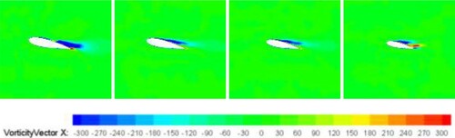
Figure 27. Axial vorticity distribution on different sections positions (the first crest, the first trough, middle, and the last trough) of the leading-edge for NSGAII01 airfoil at the stall angle 16°.

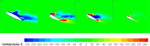
Figure 28. Axial vorticity distribution on different sections positions (the first crest, the first trough, middle, and the last trough) of the leading-edge for NSGAII02 airfoil at the stall angle 16°.

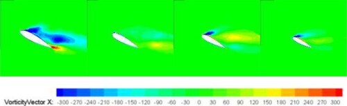
Figure 29. Axial vorticity distribution on different sections positions (the first crest, the first trough, middle, and the last trough) of the leading-edge for Kriging01 airfoil at the stall angle 16°.

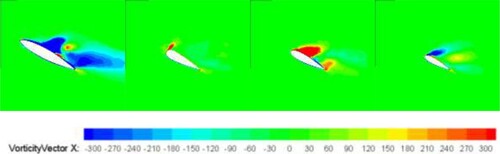
Figure 30. Axial vorticity distribution on different sections positions (the first crest, the first trough, middle, and the last trough) of the leading-edge for Kriging02 airfoil at the stall angle 14°.

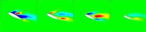
In Figures 26–30, it could be detected that with the distance away from the root of the airfoils, the distribution area of axial vorticity gradually decreases for either NACA or NSGAII01, NSGAII02, Kriging01 as well as Kriging02. In addition, on the four sections of the four optimal airfoils, lager strengths of vortices appear compared to that over NACA airfoil.

6. Conclusions

The aim of this current work is to develop a bionic wing foil inspired by the pectoral fins of humpback whales. Therefore an innovative methodology for the optimization design of the bionic airfoil with leading-edge tubercles has been explored for improving the aerodynamic performance. The three main components of an aerodynamic optimization program consisting of a wave configuration parametric design conversion module, an aerodynamic numerical solution module, and an optimization technique module are established and incorporated. For the geometry transformation, to generate variants of the frontier tubercle, F-spline curves for the parametric form method were used. A numerical study of the aerodynamic performance of the three-dimensional bionic airfoil is carried out using the Reynolds-average Navier-Stokes equation for three-dimensional non-stationary incompressibility with the γ-Reθ co-relation model has been numerically investigated. A comparison of the calculation results with the experimental results reveals a reasonable agreement, which provides a basis for the validity of the calculation results and can accordingly be used as an evaluation tool of the objective function for optimal design. The combination of Non-dominated Sorting Genetic Algorithm II and Response Surface Method based Kriging Model has been in utilization which allows a sufficient global space search. After an extensive optimization design exploration into the bio-inspired airfoil with Reynolds number 10⁵ at a wide range of the angles of attack, final four optimized designs are obtained. Compared to the smooth wing, the increments of the stall angles for four optimal airfoils which are NSGAII01, NSGAII02, Kriging01, Kriging02 run up to as much as 33.3%, 33.3%, 33.3%, 16.7% respectively and the lift has also been increased in some degree. In addition, the C_P distribution on the upper surface and the lower surface, the C_F distribution on the upper surface and the axial velocity profile as well as axial vorticity distributions contours on different sections of the airfoils have been analyzed. In conclusion, the present study reveals an effective and conservative synthesis method towards the aerodynamic optimization of airfoil design in order to delay stall and increase lift by dealing with the real bionic construction and the arrangement of the tubercles on the leading-edge, which is shown to be promising in the biomimetic exploitation fields. Based on the optimization design methodology proposed, some other constructions of the bio-inspired airfoils which are the trailing edge serrations on airfoil or wing tip tilt structure could also be explored. In a further step, the aerodynamic noise of the bio-inspired airfoil with leading-edge tubercles may be considered and improved which would be the future direction of this study.

Acknowledgments

The authors thank the reviewers for their comments and suggestions in improving the quality of the article.

Data Availability

The data used to support the findings of this study are available from the corresponding author upon request.

Disclosure statement

No potential conflict of interest was reported by the author(s).

Additional information

Funding

This work was funded by the National Natural Science Foundation of China [grant number 51809029] and the Natural Science Foundation of Liaoning Province [grant number 2019-BS-025] and the National Equipment Pre-Research Foundation of China [grant number 61402070106] and Dalian Science and Technology Innovation Fund Project [grant number 2020JJ25CY016] and the Fundamental Research Funds for the Central Universities [grant number 3132019306].

References

- Abt, C., Harries, S., Heimann, J., & Winter, H. F. (2003). Rom redesign to optimal hull line by means of parametric modeling. 2nd International on Computer Applications and Information Technology in theMarine Industries (COMPIT 2003), Hamburg, Germany, 444–458.
- Akbarian, E., Najafi, B., Jafari, M., Faizollahzadeh Ardabili, S., Shamshirband, S., & Chau, K. W. (2018). Experimental and computational fluid dynamics-based numerical simulation of using natural gas in a dual-fueled diesel engine. Engineering Applications of Computational Fluid Mechanics, 12(1), 517–534. https://doi.org/https://doi.org/10.1080/19942060.2018.1472670
- Birk, L., & Harries, S. (Eds.). (2003). OPTIMISTIC—optimization in marine design. Mensch & Buch Verlag.
- Borglund, D., & Kuttenkeuler, J. (2002). Active wing flutter suppression using a trailing edge flap. Journal of Fluids and Structures, 16(3), 271–294. https://doi.org/https://doi.org/10.1006/jfls.2001.0426
- Buchholz, M. D., & Tso, J. (2000). Lift augmentation on delta wing with leading-edge fences and Gurney Flap. Journal of Aircraft, 37(6), 1050–1057. https://doi.org/https://doi.org/10.2514/2.2710
- Cater, J. E., & Soria, J. (2002). The evolution of round zero-net-mass-flux jets. Journal of Fluid Mechanics, 472, 167–200. https://doi.org/https://doi.org/10.1017/S0022112002002264
- Choi, H. (2009). Bio-mimetic flow control. APS Division of Fluid Dynamics Meeting Abstracts.
- Corsini, A., Delibra, G., & Sheard, A. G. (2013). On the role of leading-edge bumps in the control of stall onset in axial fan blades. Journal of Fluids Engineering, 135(8). https://doi.org/https://doi.org/10.1115/1.4024115
- Deb, K., Agrawal, S., Pratap, A., & Meyarivan, T. (2000). A fast elitist non-dominated sorting genetic algorithm for multiobjective optimization: NSGA-II. Lecture Notes in Computer Science, 1917, 849–858. https://doi.org/https://doi.org/10.1007/3-540-45356-383
- Dropkin, A., Custodio, D., Henoch, C. W., & Johari, H. (2012). Computation of flow field around an airfoil with leading-edge protuberances. Journal of Aircraft, 49(5), 1345–1355. https://doi.org/https://doi.org/10.2514/1.C031675
- Favier, J., Pinelli, A., & Piomelli, U. (2012). Control of the separated flow around an airfoil using a wavy leading edge inspired by humpback whale flippers. Comptes Rendus Mécanique, 340(1-2), 107–114. https://doi.org/https://doi.org/10.1016/j.crme.2011.11.004
- Fish, F. E. (2006). Limits of nature and advances of technology: What does biomimetics have to offer to aquatic robots? Applied Bionics and Biomechanics, 3(1), 49–60. https://doi.org/https://doi.org/10.1155/2006/506474
- Fish, F. E., & Battle, J. M. (1995). Hydrodynamic design of the humpback whale flipper. Journal of Morphology, 225(1), 51–60. https://doi.org/https://doi.org/10.1002/jmor.1052250105
- Fish, F., Legac, P., Wei, T., et al. (2008). Vortex mechanics associated with propulsion and control in whales and dolphins. Comparative Biochemistry and Physiology. Part A, 3(150), S65–S66. https://doi.org/https://doi.org/10.1016/j.cbpa.2008.04.077
- Fish, F. E., Weber, P. W., Murray, M. M., Howle, L. E. (2011). The tubercles on humpback whales’ flippers: application of bio-inspired technology. https://doi.org/https://doi.org/10.1093/icb/icr016
- Grigoropoulos, G. J., & Chalkias, D. S. (2010). Hull-form optimization in calm and rough water. Journal of Computer-Aided Design, 42(11), 977–984. https://doi.org/https://doi.org/10.1016/j.cad.2009.11.004
- Hansen, K. L., Kelso, R. M., & Dally, B. B. (2011). Performance variations of leading-edge tubercles for distinct airfoil profiles. AIAA Journal, 49(1), 185–194. https://doi.org/https://doi.org/10.2514/1.J050631
- Harries, S. (1998). Parametric design and hydrodynamic optimization of ship hull forms. [Ph.D. Thesis, Institut furSchiffs-und Meerestechnik, Technische Universitat Berlin, Germany; Berlin: Mensch & Buch Verlag].
- Harries, S. (2007). Friendship systems: Hydrodynamic optimization of theDSME 60 K LPG Carrier. FS-Report, 175–02-01.
- Isaac, K., & Swanson, T. (2011). Biologically inspired wing leading edge for enhanced wind turbine and aircraft performance. AIAA Theoretical Fluid Mechanics Conferenc.
- Jeyadevi, S., Baskar, S., Babulal, C. K., & Willjuice Iruthayarajan, M. (2011). Solving multiobjective optimal reactive power dispatch using modified NSGA-II. International Journal of Electrical Power & Energy Systems, 33(2), 219–228. https://doi.org/https://doi.org/10.1016/j.ijepes.2010.08.017
- Johari, H., Henoch, C., Custodio, D., & Levshin, A. (2007). Effects of leading-edge protuberances on airfoil performance. AIAA Journal, 45(11), 2634–2642. https://doi.org/https://doi.org/10.2514/1.28497
- Kaymaz, I., & McMahon, C. A. (2005). A response surface method based on weighted regression for structural reliability analysis. Probabilistic Engineering Mechanics, 20(1), 11–17. https://doi.org/https://doi.org/10.1016/j.probengmech.2004.05.005
- Langtry, R. B. (2006). A correlation-based transition model using local variables for unstructured parallelized CFD codes. [Doctoral Thesis, University of Stuttgart].
- Lee, Y. S. (2003). Trends validation of CFD predictions for ship design purpose. [Ph. D. Thesis, Institut fur Schiffs-und Meerestechnik, Technische Universitat Berlin].
- Li, M. C., Si, Q., Liang, S. X., & Sun, Z. C. (2014). Multiple objectives for genetically optimized coupled inversionmethod for jetmodels in flowing ambient fluid. Engineering Applications of Computational Fluid Mechanics, 8(1), 82–90. https://doi.org/https://doi.org/10.1080/19942060.2014.11015499
- Liang, Y., Cheng, X. Q., Li, Z. N., & Xiang, J. W. (2011). Robust multi-objective wing design optimization via CFD approximation model. Engineering Applications of Computational Fluid Mechanics, 5(2), 286–300. https://doi.org/https://doi.org/10.1080/19942060.2011.11015371
- Maisonneuve, J. J., Harries, S., Marzi, J., Raven, H. C., Viviani, U., & Piippo, H. (2003). Toward optimal design of ship hull shapes. In: 8th international marine design conference, IMDC03, Athens.
- Mancuso, A. (2006). Parametric design of sailing hull shapes. Ocean Engineering, 33(2), 234–246. https://doi.org/https://doi.org/10.1016/j.oceaneng.2005.03.007
- Mccormick, D. C. (1993). Shock/boundary-layer interaction control with vortex generators and passive cavity. AIAA Journal, 31(1), 91–96. https://doi.org/https://doi.org/10.2514/3.11323
- Mehraban, A. A., Djavareshkian, M. H., Sayegh, Y., Feshalami, B. F., & Hassanalian, M. (2020). Effects of smart flap on aerodynamic performance of sinusoidal leading-edge wings at low reynolds numbers. Proceedings of the Institution of Mechanical Engineers Part G-Journal of Aerospace Engineering, No. 0954410020946903.
- Menter, F. R., Langtry, R. B., et al. (2004). A correlation-based transition model using local variables Part 1 - Model Formulation. Proc. ASME Turbo Expo, June 14-17, Vienna, Austria. https://doi.org/https://doi.org/10.1115/gt2004-53452
- Miklosovic, D. S., Murray, M. M., & Howle, L. E. (2007). Experimental evaluation of sinusoidal leading edges. Journal of Aircraft, 44(4), 1404–1408. https://doi.org/https://doi.org/10.2514/1.30303
- Pérez, F., & Clemente, J. A. (2011). Constrained design of simple ship hulls with B-spline surfaces. Computer-Aided Design, 43(12), 1829–1840. https://doi.org/https://doi.org/10.1016/j.cad.2011.07.008
- Peri, D., Rossetti, M., & Campana, E. F. (2001). Design optimization of ship hulls via CFD techniques. Journal of Ship Research, 45(2), 140–149. https://doi.org/https://doi.org/10.1016/S1385-1101(01)00059-4
- Post, M. L., & Corke, T. C. (2004). Separation control on high angle of attack airfoil using plasma actuators. AIAA Journal, 42(11), 2177–2184. https://doi.org/https://doi.org/10.2514/1.2929
- Ramezanizadeh, M., Nazari, M. A., Ahmadi, M. H., & Chau, K. (2019). Experimental and numerical analysis of a nanofluidic thermosyphon heat exchanger. Engineering Applications of Computational Fluid Mechanics, 13(1), 40–47. https://doi.org/https://doi.org/10.1080/19942060.2018.1518272
- Rao, D. M., & Campbell, J. F. (1987). Vortical flow management techniques. Progress in Aerospace Sciences, 24(3), 173–224. https://doi.org/https://doi.org/10.1016/0376-0421(87)90007-8
- Ren, W. X., & Chen, H. B. (2010). Finite element model updating in structural dynamics by using the response surface method. Engineering Structures, 32(8), 2455–2465. https://doi.org/https://doi.org/10.1016/j.engstruct.2010.04.019
- Saha, G. K., Suzuki, K., & Kai, H. (2004). Hydrodynamic optimization of ship hull forms in shallow water. Journal of Marine Science and Technology, 9, 51–62. https://doi.org/https://doi.org/10.1007/s00773-003-0173-3
- Sakata, S., Ashida, F., & Zako, M. (2004). An efficient algorithm for Kriging approximation and optimization with large-scale sampling data. Computer Methods in Applied Mechanics and Engineering, 193(3), 385–404. https://doi.org/https://doi.org/10.1016/j.cma.2003.10.006
- Salih, S. Q., Aldlemy, M. S., Rasani, M. R., Ariffin, A. K., Ya, T. M. Y. S. T., Al-Ansari, N., Yaseen, Z. M., & Chau, K. W. (2019). Thin and sharp edges bodies-fluid interaction simulation using cut-cell immersed boundary method. Engineering Applications of Computational Fluid Mechanics, 13(1), 860–877. https://doi.org/https://doi.org/10.1080/19942060.2019.1652209
- Seifert, A., Bachar, T., Koss, D., Shepshelovich, M., & Wygnanski, I. (1993). Oscillatory blowing: A tool to delay boundary-layer separation. AIAA Journal, 31(11), 2052–2060. https://doi.org/https://doi.org/10.2514/3.49121
- Seifert, A., Darabi, A., & Wyganski, I. (1996). Delay of airfoil stall by periodic excitation. Journal of Aircraft, 33(4), 691–698. https://doi.org/https://doi.org/10.2514/3.47003
- Shi, W., Atlar, M., Norman, R., Aktas, B., & Turkmen, S. (2016). Numerical optimization and experimental validation for a tidal turbine blade with leading-edge tubercles. Renewable Energy, 96, 42–55. https://doi.org/https://doi.org/10.1016/j.renene.2016.04.064
- Shormann, D. E., & Panhuis, M. I. H. (2019). Performance evaluation of a humpback whale-inspired hydrofoil design applied to surfboard fins. MTS/IEEE Oceans Seattle Conference, Seattle, Marine Technol Soc; IEEE.
- Srinivas, N., & Deb, K. (1994). Muiltiobjective optimization using nondominated sorting in genetic algorithms. Evolutionary Computation, 2(3), 221–248. https://doi.org/https://doi.org/10.1162/evco.1994.2.3.221
- Stanway, M. J. (2008). Hydrodynamic effects of leading-edge tubercles on control surfaces and in flapping foil propulsion. Massachusetts Institute of Technology.
- Tae, H. J., Shin, Y. J., Kim, B. J., & Kim, M. (2017). A numerical performance study on rudder with wavy configuration at high angles of attack. Journal of The Society of Naval Architects of Korea, 54(1), 18–25. https://doi.org/https://doi.org/10.3744/SNAK.2017.54.1.18
- Tuck, A., & Soria, J. (2004). Active flow control of a NACA 0015 airfoil using a ZNMF jet. Australian Aerospace Student Conference, Sydney.
- Tunio, I. A., Kumar, D., & Hussain, T. (2020). Investigation of variable spanwise waviness wavelength effect on wing aerodynamic performance. Fluid Dynamics, 55(5), 657–669. https://doi.org/https://doi.org/10.1134/S0015462820040102
- Valorani, M., Peri, D., & Campana, E. F. (2003). Sensitivity analysis techniques for design optimization ship hulls. Optimization and Engineering, 4(4), 337–364. https://doi.org/https://doi.org/10.1023/B:OPTE.0000005391.23022.3b
- Vipperman, J. S., Clark, R. L., Conner, M., & Dowell, E. H. (1998). Experimental active control of a typical section using a trailing-edge flap. Journal of Aircraft, 35(2), 224–229. https://doi.org/https://doi.org/10.2514/2.2312
- Wang, J., Li, Y., & Choi, K. (2008). Gurney flap—lift enhancement, mechanisms and applications. Progress in Aerospace Sciences, 44(1), 22–47. https://doi.org/https://doi.org/10.1016/j.paerosci.2007.10.001
- Watts, P., & Fish, F. E. (2001). The influence of passive, leading edge tubercles on wing performance.Proc. Twelfth Intl. Symp. Unmanned Untethered Submers. Technol. Durham New Hampshire: Auton. Undersea Syst. Inst.
- Weber, P. W., Howle, L. E., & Murray, M. M. (2010). Lift, drag, and cavitation onset on rudders with leading-edge tubercles. Marine Technology, 47(1), 27–36. https://doi.org/https://doi.org/10.1080/1064119X.2010.532390
- Yasuda, T., Fukui, K., Matsuo, K., Minagawa, H., & Kurimoto, R. (2019). Effect of the Reynolds number on the performance of a NACA0012 wing with leading edge protuberance at Low Reynolds numbers. Flow, Turbulence and Combustion, 102(2), 435–455. https://doi.org/https://doi.org/10.1007/s10494-018-9978-3
- Yoon, H. S., Hung, P. A., Jung, J. H., & Kim, M. C. (2011). Effect of the wavy leading edge on hydrodynamic characteristics for flow around low aspect ratio wing. Computers & Fluids, 49(1), 276–289. https://doi.org/https://doi.org/10.1016/j.compfluid.2011.06.010
- Zhang, J., Huang, H. W., & Phoon, K. K. (2013). Application of the Kriging-based response surface method to the system reliability of soil slopes. Journal of Geotechnical and Geoenvironmental Engineering, 139(4), 651–655. https://doi.org/https://doi.org/10.1061/(ASCE)GT.1943-5606.0000801