Improved method for identifying Manning’s roughness coefficients in plain looped river network area

Abstract

Manning’s roughness coefficient(n) is considered a key parameter in a one-dimensional (1D) hydrodynamic model. However, it is highly variable and time- and site- dependent. Further, identifying proper n values is not easy, especially in plain looped river network areas. Therefore, a more systematic approach is needed. This study proposes a coupled optimization-simulation model to systematically estimate the spatial distribution of n values. The particle swarm optimization (PSO) algorithm and InfoWorks Integrated Catchment Modelling (ICM) software were integrated to solve the objective function and hydraulic process, respectively. Crisscrossing rivers were partitioned into river reaches that were each assumed to have a uniform and constant Manning’s roughness coefficient according to their network topology and cross-section variation. In addition, a sensitivity analysis was implemented to determine the weights of measured data from different gauging stations, and a large difference in the spatial distribution of the sensitivity index illustrated the importance of identifying the weights of multiple stations. Then, a systematic approach was applied to estimate the n values in the Changshu Grand Polder Area (CGPA), which is crisscrossed by 150 rivers, under the water diversion stage. The calculation statistics and efficiency indicated that the proposed method performs well for model calibration.

KEYWORDS:

• Manning’s roughness coefficient
• plain looped river network area
• particle swarm optimization (PSO)
• sensitivity analysis
• Latin hypercube sampling (LHS)
• InfoWorks integrated Catchment Modelling (ICM)

1. Introduction

Hydrodynamic models have been widely used in applications such as water resource management and water conservancy project design and impact evaluation (Hadiyanto et al., 2013; Neumayer et al., 2020; Pasternack et al., 2004). The accuracy, stability, and robustness of a hydrodynamic model are affected not only by the detailed basic data used for model development but also by the use of suitable model parameters. Among various model parameters, Manning’s roughness coefficient (n), an integrated dimensionless number, is considered a key parameter that has a significant influence on the flow discharge and water level (Choo et al., 2018; Li & Zhang, 2001). It also reflects the influence of flow resistance, which has a real physical interpretation (Chow, 1959; Cowan, 1956).

Many manuals have provided guidance on the selection of Manning’s roughness coefficient in the form of photographs, tables, etc. (Arcement & Schneider, 1989; Barnes, 1967; Chow, 1959, 1988). However, the value of this empirical parameter not only depends on various factors such as river irregularities, cross-section variations, meandering, vegetation, obstructions, and bed material, but also varies with the effect of unsteadiness (Choo et al., 2018; Chow, 1959; De Doncker et al., 2009; Ding & Wang, 2005). Further, these resistance factors vary along the river, making it difficult to quantify the n values. Therefore, many studies have emphasized the importance of model calibration for estimating n values (Andréassian et al., 2009; Gupta et al., 1999; Kirchner, 2006). In fact, most mathematical models need to be calibrated before practical applications (Gupta et al., 1998; Malaterre et al., 2010). Detailed measurement data can be used to identify the distribution of n-values by hydrodynamic model calibration (Orlandini, 2002).

In practice, global (Parhi et al., 2012; Timbadiya et al., 2011) and spatially varying n values (Attari & Hosseini, 2019; Jahandideh-Tehrani et al., 2020; Ong et al., 2017) are commonly used in model calibration. It is simple and effective to take a global roughness value for a few rivers having similar cross-sections without floodplains under the condition of limited water level change. In this case, the distribution of n values is usually estimated through trial-and-error based on the measured water level or flow hydrographs (Boulomytis et al., 2017; Hameed & Ali, 2013; Parhi et al., 2012). Specifically, the observed and the simulated data are visually compared until the discrepancy between these two datasets is acceptable. However, the accuracy of this manual parameter estimation procedure mainly depends on the experience of the modelers (Ayvaz & Genç, 2012). For a general river network, cross-sections could vary across different rivers and even at different locations along a single river. In addition, a significant difference in roughness can be found between the main river and the floodplain. The roughness can also vary with depth (Chow, 1959). Therefore, the application of spatially varying n values is more accurate and suitable in a general river network. However, the use of spatially varying n values could significantly increase the number of possible roughness sets and thereby incur high calibration workloads (Ayvaz, 2013). In addition, any adjustment of n values may lead to unpredictable water level or flow behaviors in a complicated river network (Kurnatowski, 2013; Ong et al., 2017).

In this context, a more systematic estimation approach is necessary. To overcome the disadvantages of the manual trial-and-error approach, automatic calibration procedures integrated with optimization algorithms have attracted considerable attention in recentyears (Ayvaz & Genç, 2012; Bekele & Nicklow, 2007; Duan et al., 1993; Madsen, 2003; Ong et al., 2017). Most previous studies usedgradient-based optimization algorithms to obtain n values (Ding et al., 2004; Fabio et al., 2010; Ramesh et al., 2000). These algorithms afford advantages such as high convergence rate, computational stability, and efficiency when searching for global solutions. Gradient-based methods must have the gradient information of the objective functions; therefore, the solution quality mostly depends on the initial parameter values (Lacasta et al., 2017). In addition, these methods need to assume the objective functions and parameters to be smooth and continuous in the search space. Therefore, such problems should preferentially be solved using metaheuristic optimization algorithms that can overcome the abovementioned limitations.

Although metaheuristic optimization algorithms have been broadly applied in various research areas (Fong et al., 2015; Holden & Freitas, 2008; Yao et al., 2015; Zeng et al., 2017), only a few studies have used them to estimate Manning’s roughness coefficients. For example, Ong et al. (2017) proposed a simulated annealing algorithm as an optimizer to calibrate the roughness coefficients of a river network with 29 channels. During optimization, the roughness of each channel was assumed to be a constant value within the range of 0.03–0.05. Ayvaz and Genç (2012) integrated the Hydrologic Engineering Center’s River Analysis System (HEC-RAS) and the Harmony Search algorithm to determine the spatial distribution of the roughness parameters of three reaches within a single channel for with and without measurement errors. Ayvaz (2013) proposed a model that combined HEC-RAS and the particle swarm optimization (PSO) algorithm to estimate the n values and their associated parameter structures for a single river. In addition, the parameter structure of a given single river was partitioned into subregions using a the one dimensional (1D) Voronoi diagram. Yang et al. (2014) proposed a system that integrated the HEC-RAS and a micro genetic algorithm and verified its ability to estimate the roughness coefficients under high- and low-flow events.

However, the abovementioned studies mainly used metaheuristic optimization algorithms integrated with simulation models for estimating the n values of a single river. To the best of our knowledge, no study has used a metaheuristic optimization algorithm integrated with a simulation model to estimate the roughness distribution of natural water courses in plain looped river network areas. Plain looped river networks differ from a dendritic river network in four aspects: substantial rivers, stronger river structure connectivity, considerable pump stations and sluice structures, and abundant gauging stations for monitoring water levels. Any localized alteration in a plain looped river network may lead to unpredictable changes in water level or flow in other remote regions (Kurnatowski, 2013). A large number of rivers increase the dimension of the n values to be calibrated. In addition, few studies have discussed the application of multisite measurement data to improve the calibration accuracy. Therefore, a more systematic approach is needed to estimate the roughness parameters of natural rivers in plain-looped river network areas.

This study proposes an optimization-simulation model that can be used to systematically estimate the roughness parameter structure and the n values of each river reach in a plain looped river network area. Sensitivity analysis was implemented to determine the weights of different gauging stations to formulate the objective function. In this study, the PSO algorithm and InfoWorks Integrated Catchment Modelling (ICM) software were chosen to solve the objective function and simulate the hydrodynamic process respectively. The rest of this paper is structured as follows. Section 2 introduces the study area and different types of datasets and explains the model calibration framework and evaluation criteria. Section 3 presents the results and discussion. Finally, Section 4 presents the conclusions of this study.

2. Materials and methods

2.1. Study area and datasets

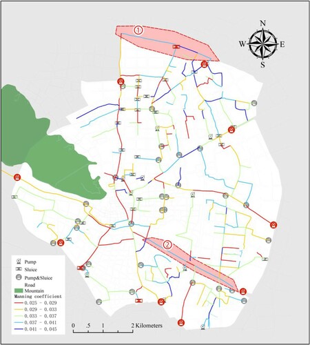
This study was conducted in the Changshu Grand Polder Area (CGPA; area: 60.7 km²), Taihu Basin, in Changshu, a county-level city in Suzhou city in China. Figure 1 shows the location of the study area and the rivers, pumps, sluices and gauging stations within it; the CGPA is enclosed by dikes and contains 23 water conservancy projects, with the main pumps and sluices marked in red. The seasonal water level variation in the CGPA is small and is controlled within the range of 3.0–3.6 m through these water conservancy projects. In addition, the CGPA is a typical plain river network area that is crisscrossed by 150 rivers with a length of ∼138 km. The rivers have a width of 10–80 m. Almost all rivers have typical artificial U-shaped sections in the main channel with no floodplains in the study area and a water depth of 2.5–3.5 m. There is little vegetation in the urban river course of the study area. However, the many bridges across the river could affect the local roughness. In addition, the average slope of the rivers in the CGPA is ∼0.00052. The river flow can be 4–30 m³/s during floods. The flow interaction between rivers was usually weak in this region owing to the smaller slope of the rivers and the closure of the water conservancy projects in nonflood periods. It should be noted that the water conservancy projects have recently been used to increase water flow to protect the environment in nonflood periods. In this study, n values are determined based on this water diversion stage. (Table 1).

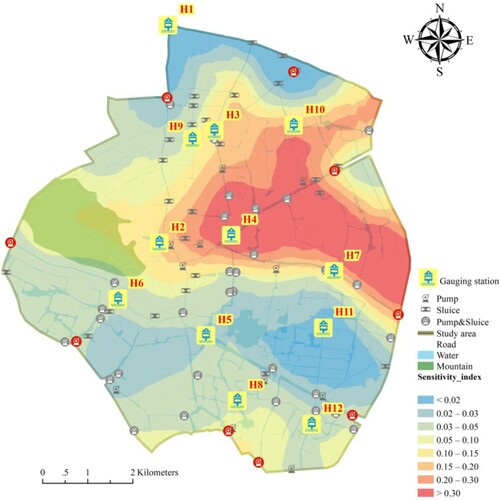
Figure 1. Location of the study area and the spatial distribution of rivers, pumps, sluices, and gauging stations. The main water conservancy projects at the boundary of the CGPA are marked in red. Gauging stations are of two types: B1 to B8 and H1 to H12. The water-level time series data measured by these two types of stations are used for providing boundary conditions for the model simulations and for calibrating the Manning’s roughness coefficients by minimizing the overall discrepancies between the simulated and the measured data, respectively.

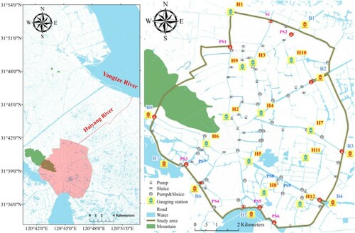
Table 1. Summary of dataset series and sources.

Dataset type	Application	Dataset resolution	Source
Cross-sectional data	Model development	One survey section at 100-m intervals	Changshu Water Bureau
Water conservancy project data	Model development	Location and properties of each project	Changshu Water Bureau
Water-level time series data	Model calibration	Automatically measured every 15 min	Water gauging stations during experiment from Changshu Water Bureau
Water conservancy project operation data	Model calibration	Automatically recorded during each operation	Real-time system during experiment from Changshu Water Bureau

The study data are divided into model development and model calibration datasets. The former includes cross-sectional data, properties, and locations of water conservancy projects and rivers that were obtained from the Changshu Water Bureau. Within the scope of this study, we primarily use the latter datasets for estimating n values.

Two main types of datasets are required for model calibration. The first type is water-level time series data that are automatically measured by water gauging stations every 15 min. In this study, such data measured by gauging stations B1 to B8 and H1 to H12 were used for providing boundary conditions for the model simulations and for calibrating n values, respectively. The second type of dataset is operation data that are monitored and recorded by the real-time system. To some degree, accurate operation data are extremely important, especially in a polder area with many pumping stations and sluice structures.

An experiment was conducted in the absence of rainfall to obtain these two types of datasets for calibration on May 23–25, 2019. During the experiment, water was drained from the Yangtze River into the Haiyang River by a pumping station and sluice structure from 7:00 am to 16:00 pm every day. Then, the water was transported through the Haiyang River to the northern part of the CGPA. Subsequently, the water flowed into the CGPA through three main structures (PS1, S1 and PS2). Finally, water was pumped out by four pumping stations (PS3, PS4, PS5 and PS6) from 8:00 am to 18:00 pm daily. Furthermore, to ensure the safety of a few low-lying areas, some pumping stations, including PS7, PS8, and PS9, were operated during the experiment. Additionally, other pumps were closed and the sluices were fully opened during the entire experimental period. During the experiment, the water level was controlled within the range of 3.2–3.6 m.

2.2. Model calibration framework

2.2.1. Particle swarm optimization

In this study, the PSO algorithm, a popular metaheuristic search algorithm, is used for estimating n values along the flow reach. The PSO algorithm was first developed in 1995 by Kennedy and Eberhart (Kennedy & Eberhart, 1995). Since then, it has attracted much interest in different disciplines and has been applied broadly to various research areas such as function optimization (Wang et al., 2019; Yao et al., 2015), data mining (Fong et al., 2015; Holden & Freitas, 2008; Van der Merwe & Engelbrecht, 2003), and machine learning (Tayfur et al., 2018; Zeng et al., 2017). The main benefits of PSO algorithm are its low computational burden and promising performance (Fotovatikhah et al., 2018). This optimization technique is inspired by the natural swarm collective behavior seen in a flock of birds or a school of fish. In the PSO algorithm, each particle can be considered a potential solution to a given problem in the defined search space. All individuals have a position, velocity, and fitness determined by the objective function. Further, the ‘swarm’ and each ‘particle’ remember the global best position and individual best position in each calculation, respectively.

The main steps in the PSO algorithm are summarized below.

• Step 1: Initialize the particle swarm with a population of random feasible solutions. Each individual has a position $P_i=(x_{i,1},x_{i,2},\dots ,x_{i,D})$ and a velocity $V_i=(\mathrm{\Delta }{x}_{i,1},\mathrm{\Delta }{x}_{i,2},\dots ,\mathrm{\Delta }{x}_{i,D})$ in the D-dimensional search space.

• Step 2: Calculate the fitness of each individual in the population using the objective function.

• Step 3: Determine the individual best fitness (P_best) for each individual and the global best fitness (G_best). For every iteration, the current position of each particle is compared with its previous best position. If the fitness of the current position is higher, the historical best position is updated to the current position. In addition, P_best for each particle is compared with the previous G_best to update G_best with the greatest fitness.

• Step 4: Update the position and velocity of each particle using Equations (1) and (2). (1) $\begin{array}{rl}{V}_i^{k+1}& =\omega V_i^k+C_1{R}_1(P_{\text{best},i}^k-P_i^k)\\ & +C_2{R}_2(G_{\text{best}}^k-P_i^k)\end{array}$(1) (2) $\begin{array}{rl}{P}_i^{k+1}& =P_i^k+V_i^{k+1}\end{array}$(2)

Subject to: (3) $V_{min}\le V_i^{k+1}\le V_{max}$(3) (4) $P_{min}\le P_i^{k+1}\le P_{max}$(4)

• Step 5: Repeat steps 2–4 until a termination criterion (e.g. maximum iterations) is reached.

The parameters of the algorithm are as follows:

• $V_i^k$ is the velocity vector of the i-th particle in the k-th iteration.

• $V_{\text{min}}$ and $V_{\text{max}}$ are the minimum and maximum velocity vector respectively.

• $P_i^k$ represents the the position vector of the i-th particle in the k-th iteration.

• $P_{\text{min}}$ and $P_{\text{max}}$ are the minimum and maximum position vector respectively.

• $P_{\text{best},i}^k$ and $G_{\text{best}}^k$are the best i-th particle position vector and best group position vector respectively.

• $R_1$ and $R_2$ are two random vectors generated uniformly from the range [0,1].

• $\omega$ denotes the inertia weight that represents the contribution of the previous velocity of an individual to its velocity in the current iteration. $\omega$ is an important parameter that can influence the performance of the PSO algorithm. A larger inertia weight value is expected to improve the exploration characteristics of the PSO algorithm; a smaller value results in exploitation in the local search. The inertia weight can be set to fixed (Shi & Eberhart, 1998), linearly time-varying (Shi & Eberhart, 1999), nonlinear-time varying (Li et al., 2009), or fuzzy adaptive (Bajpai & Singh, 2007) values. In this study, the widely used approach of linearly decreasing the inertia weight was chosen to set the inertia weight owing to its efficiency and simplicity. The ${\omega }_{\text{min}}$ and ${\omega }_{\text{max}}$ values are widely set as 0.4 and 0.9, respectively (Rezaee Jordehi & Jasni, 2013; Sengupta et al., 2018).

• $C_1$ and $C_2$ are learning parameters that represent the cognitive learning rate and social learning rate, respectively. These parameters represent the weights that pull particles toward the cognitive attractor ($P_{\text{best},i}^k$) and social attractor ($G_{\text{best}}^k$), respectively. The PSO algorithm is likely to not converge when the values of these parameters are too low; however, much higher values could cause the particles to move abruptly. $C_1$ = $C_2$ = 2 is the setting that has been widely used in many practical applications, and it is considered acceptable for mostthe problems (Ozcan & Mohan, 1999). (Table 2).

Table 2. Summary of parameter settings in optimization model and statistics of simulation model.

Optimization model		Simulation model
Particle population	20	Number of pumping stations	59
Number of generations	400	Number of sluice structures	71
${\omega }_{min};{\omega }_{max}$	0.4; 0.9	Number of river-reaches	313
${\text{C}}_1$; ${\text{C}}_2$	2; 2	Number of cross-sections	1060
$v_{min}$; $v_{max}$	−0.002; 0.002	Length of simulated river network (km)	138
$p_{min}(n_{min})$; $p_{max}(n_{max})$	0.025; 0.045	Boundaries	8

2.2.2. Simulation model

In this study, a 1D unsteady hydrodynamic model was developed for the looped river network using the InfoWorks ICM software, a well-known integrated modeling platform that incorporates hydraulic and hydrological modeling (Peng et al., 2016, 2015). The simulation conditions satisfy the basic assumptions of Saint-Venant equations such as fixed channel geometry, homogeneous fluid, and narrow channel slope. In this software, gradually varying unsteady flow simulations are based on Saint-Venant equations (Yen, 1973). The Preissmann four -point scheme is used to solve these equations. (5) $\begin{array}{rl}& \frac{\mathrm{\partial }A}{\mathrm{\partial }t}+\frac{\mathrm{\partial }Q}{\mathrm{\partial }x}=q\end{array}$(5) (6) $\begin{array}{rl}& \frac{\mathrm{\partial }Q}{\mathrm{\partial }t}+\frac{\mathrm{\partial }(Q^2/A)}{\mathrm{\partial }x}+gA\frac{\mathrm{\partial }h}{\mathrm{\partial }x}+gA(S_0-S_f)=0\end{array}$(6) (7) $\begin{array}{rl}& S_f=\frac{n^{2}Q|Q|}{A^2{R}^{4/3}}\end{array}$(7) where A is the cross-sectional area perpendicular to the flow (m²); Q, the discharge (m³/s); q, the lateral inflow (m³/s); t, the time (s); x, the distance along the channel from the reference point (m); g, the acceleration due to gravity (m/s²); h, the water level above the datum in the channel (m); S₀, the bed slope (m/m); S_f, the friction slope (m/m); R, the hydraulic radius (A/P) (m); P, the wetted perimeter at the cross-sectional position (m); and n, Manning’s roughness coefficient, which is commonly determined by model calibration.

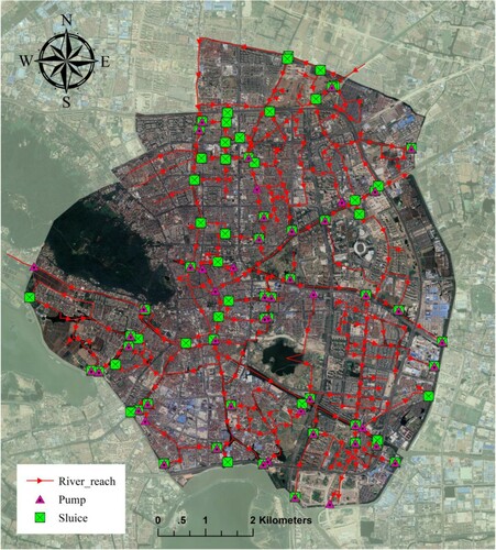
Figure 2 shows the developed model structure consisting of 313 river reaches, 59 pumping stations, 71 sluice structures, and 1060 cross-sections. To reduce the complexity of the search space, each river reach is assumed to have a uniform and constant Manning’s roughness coefficient. This hypothesis is feasible because of the similar cross-sectional geometry with no floodplains and limited water variation in this area. Eventually, 150 rivers were partitioned into 313 river reaches by (1) dividing at the junction of rivers, (2) separating at pumps or sluices, (3) splitting at large cross-section variations in a river. The pumps and sluices were built to connect the river reaches based on the actual situation. The basic properties of sluices, such as the width and invert level, are fixed. The discharge of pumps and opening height of sluices varied with time during the simulation period. During model calibration, the operation data were monitored and recorded by a real-time system.

Figure 2. 1D dynamic model structure of the river networks in the study area as built using InfoWorks ICM software.

The model domain contains eight open boundaries, B1 to B8 (Figure 1). The water-level time series data measured automatically by gauging stations every 15 min were used to provide the boundary conditions during model calibration. Before the experiment, the initial level was constant owing to the closure of the water conservancy projects. Therefore, the initial water level in the model domain was set to a fixed measured value of 3.33 m. Considering the numerical stability, accuracy, and computing speed, the time step of the simulation was set as 60 s. The time step of the simulation results was set to 15 min, which is the same as the measurement time step, to save storage capacity. (Table 3).

Table 3. Statistical parameters of NSE and SI calculated from sensitivity analysis (SD: standard deviation; CV: coefficient of variation).

	Gauging station
Statistical parameters	H1	H2	H3	H4	H5	H6	H7	H8	H9	H10	H11	H12
Mean of NSE	0.013	0.074	0.073	0.183	0.024	0.059	0.17	0.022	0.043	0.087	0.02	0.026
SD of NSE	0.002	0.033	0.03	0.077	0.01	0.015	0.102	0.015	0.014	0.057	0.006	0.009
CV of NSE	13.32	44.15	41.03	41.76	40.96	25.88	60.09	67.34	32.38	65.12	31.21	34.79
Normalized SI	0.004	0.074	0.079	0.256	0.018	0.032	0.311	0.028	0.036	0.133	0.009	0.02

2.2.3. Formulation of objective function

This study aims to estimate Manning’s roughness coefficient of the river network in the study area. This objective can be mathematically solved by integrating the optimization and simulation models. Thus, an objective function is required to minimize the discrepancies between the observed and the simulated water levels at the 12 gauging stations, H1 to H12 (Figure 1), during the experiment. Several studies have illustrated the importance of choosing suitable objective functions (Efstratiadis & Koutsoyiannis, 2010; Her & Seong, 2018). Commonly, model performance evaluation metrics are used as objective functions (Brighenti et al., 2019; Dung et al., 2010; Foulon & Rousseau, 2018; Jiang et al., 2020; Ong et al., 2017). In this study, the Nash–Sutcliffe Efficiency (NSE) (Nash & Sutcliffe, 1970), which was commonly used in previous studies, was chosen as the objective function for each gauging station. The NSE can range from −∞ to 1. Some studies classified NSE values of (0.75, 1], (0.65, 0.75], (0.5, 0.65], and (−∞, 0.5] as very good, good, satisfactory, and unsatisfactory, respectively. Additionally, to simplify the optimization problem, 12 objective functions were converted to a single objective function (Equation (8)). (8) $\begin{array}{rl}& \text{Maximize: Objective function}\\ & =1-\sum _{i=1}^N{\theta }_i\frac{{\sum }_{t=1}^T{\phi }_t{(Z_{\text{obs},i}^t-Z_{\text{sim},i}^t)}^2}{{\sum }_{t=1}^T{\phi }_t{(Z_{\text{obs},i}^t-\overline{Z_{\text{obs},i}})}^2}\end{array}$(8) With $\sum _{i=1}^N{\theta }_i=1$ and subject to (9) $n_{min}\le n\le n_{max}$(9) The parameters of the objective function are as follows:

1. $Z_{obs,i}^t$ and $Z_{\text{sim},i}^t$ are the measured and simulated values at the t-th time step and i-th gauging station, respectively. $\overline{Z_{\text{obs},I}}$ is the average of measured values at the i-th gauging station.

2. T and N are the number of time steps and gauging stations in the calibration period, respectively.

3. $n_{min}$ and $n_{max}$ are the lower and upper bounds of the n values of each river reach, respectively. In this study, almost all rivers had typical artificial U-shaped sections in the main channel with no floodplains in the city and a water depth of 2.5–3.5 m. A feasible range of n values was chosen based on hydraulics textbooks (Arcement & Schneider, 1989; Barnes, 1967; V. T. Chow, 1988) and a field prototype experiment (Huang & Xiang, 2017). Furthermore, the range was expanded slightly to compensate for the model errors (e.g. geometric errors, model dimensions, etc.). The lower and upper bounds of the roughness coefficients were set as 0.025 and 0.045, respectively.

4. ${\phi }_t$ is the weighting coefficient at the t-th time step. Actually, it is difficult to obtain a model that can achieve equal performance for high and low flows or water levels. Therefore, this weighting coefficient can be used to highlight some given partitions of the hydrograph according to the research objective. This study focused on theoperation period of pumping stations within the study area (8:00 am to 18:00 pm daily). In fact, the setting of ${\phi }_t$ involves some subjectivity based on the experience of the modelers. Finally, this weighting coefficient was set as 0.8 during the operation period and 0.2 during the nonoperation period.

5. ${\theta }_i$ is the weight of the i-th gauging station. This parameter indicates the different importance of each gauging station based on two facts. One is that the measured data from different gauging stations have different accuracy and reliability. The other is that the model structure and boundary conditions impact the simulated water level at gauging stations. In this study, it is assumed that the measured data from gauging stations have the same accuracy and reliability. Therefore, the weights of gauging stations were mainly based on the model structure and boundary conditions. A sensitivity analysis was conducted to determine the impact of the n value distribution on the fitness of each gauging station.

It is well known that the sensitivity can be analyzed by two main approaches: local sensitivity analysis and global sensitivity analysis. The former approach is sometimes known as the one-at-a-time (OAT) method; it analyzes the influence of one parameter on the objective at a time while keeping other parameters fixed. Local sensitivity analysis is widely used in many fields. Global sensitivity analysis is more useful for problems with large parameters under a limited number of simulations (van Griensven et al., 2006). Globally possible roughness sets in the design space were sampled by Latin hypercube sampling (LHS) (McKay et al., 1979), which is based on a high-efficiency Monte Carlo method. In this study, 4000 roughness coefficient sets within the range of 0.025–0.045 were generated by LHS for 313 river reaches to conduct global sensitivity analysis. The sensitivity index (SI) is defined as the ratio between the difference and the sum of the maximum and the minimum NSEs (Equation (10)) (Jiang et al., 2020), and it is calculated to evaluate the sensitivity of each gauging station for all n value sets. In this study, the SI was also used to represent the weight of the gauging station, $\theta$. (10) $\text{Sensitivity Index}=\frac{\text{Ma}{\text{x}}_{\text{NSE}}-\text{Mi}{\text{n}}_{\text{NSE}}}{\text{Ma}{\text{x}}_{\text{NSE}}+\text{Mi}{\text{n}}_{\text{NSE}}}$(10) A parameter is considered more sensitive than another if the SI is closer to 1.

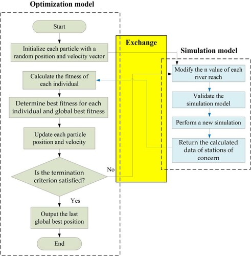
As indicated in the previous section, the 1D hydrodynamic model was developed using the InfoWorks ICM software, and the roughness parameter structure was estimated using the PSO algorithm. For each iteration, a simulation model is executed to modify the roughness of each river reach and simulate the hydrodynamic response to the n value structure. In the optimization model, the objective function fitness is calculated, and then, a more appealing roughness set is chosen. Thus, it is necessary to integrate the optimization model and simulation model in one platform. In this study, an optimization-simulation model developed in Ruby was compiled to run on a Windows system. Note that ICM Exchange is used to exchange data between the InfoWorks ICM software and the PSO algorithm. Figure 3 shows a general flowchart of the optimization-simulation model.

Figure 3. General flowchart of optimization-simulation model.

2.3. Evaluation criteria

Model performance metrics are often used during model calibration (Gholami et al., 2016; Shamshirband et al., 2018). The three well-known statistical metrics used in this study are (1) NSE (Nash & Sutcliffe, 1970), (2) Pearson’s correlation coefficient (R), and (3) percent bias (PBIAS) (Yapo et al., 1996). The equation and performance rating of the NSE have been presented in the previous subsection. The latter two criteria are described in detail in this subsection.

Pearson’s correlation coefficient is a measure of the linear relationship between two variables. It is often used to calculate the linear correlation between the flow process and the water level process of the hydrodynamic simulation results. It is calculated as follows: (11) $R=\frac{\begin{array}{c}T{\sum }_{t=1}^T{Z}_{\text{obs}}^t{Z}_{\text{sim}}^t\\ -{\sum }_{t=1}^T{Z}_{\text{obs}}^t{\sum }_{t=1}^T{Z}_{\text{sim}}^t\end{array}}{\begin{array}{c}\sqrt{T{\sum }_{t=1}^T{(Z_{\text{obs}}^t)}^2-{\left({\sum }_{t=1}^T{Z}_{\text{obs}}^t\right)}^2}\\ \sqrt{T{\sum }_{t=1}^T{(Z_{\text{sim}}^t)}^2-{\left({\sum }_{t=1}^T{Z}_{\text{sim}}^t\right)}^2}\end{array}}$(11) where $Z_{\text{obs}}^t$ and $Z_{\text{sim}}^t$ are respectively the measured and simulated values at the t-th time step, and T is the number of time steps. The larger the absolute value of R, the stronger is the correlation. The values of this metric range from −1 (strong negative relationship) to 1 (strong positive relationship). Values of or close to zero imply a weak or no linear relationship.

The percent bias is often used to measure the tendency of the relationship between the simulated and the observed values. The ideal value of PBIAS is 0%. Positive and negative values indicate model underestimation and overestimation, respectively. (12) $\text{PBIAS}=\frac{{\sum }_{t=1}^T(Z_{\text{obs}}^t-Z_{\text{sim}}^t)}{{\sum }_{t=1}^T{Z}_{\text{obs}}^t}\times 100$(12) where $Z_{\text{obs}}^t$ is the observed value at the t-th time step, and $Z_{\text{sim}}^t$ is the simulated value at the t-th time step.

3. Results and discussion

3.1. Sensitivity analysis

As indicated previously, 4000 roughness sets sampled by LHS within the range of 0.025–0.045 were realized using the InfoWorks ICM software. Figure 4 shows the results of the sensitivity analysis of the roughness structure of the 12 gauging stations. The violin plots reveal a large difference between the NSE value of each gauging station. H4 and H7 are listed in the first two gauging stations with large NSE values of0.58 and 0.69, respectively; they have good average NSE values of 0.82 and 0.83, respectively, but minimum NSE values of 0.32 and 0.25, respectively. These smaller values indicate that the roughness structure has a great impact on H4 and H7 with this calibration model and boundary conditions. In contrast, the smallest range of NSE with H1 implies that this gauging station was only slightly affected by the variation in the roughness sets. In addition, the remaining stations show similar probability densities. Overall, the average NSE of each gauging station is not significant within the range of 0.85–0.97. The SI of each gauging station as calculated using by Equation (7) is indicated by the red line with triangle markers in Figure 4. The difference between these SI is very large. The normalized SI for the 12 stations are 0.004, 0.074, 0.079, 0.256, 0.018, 0.032, 0.311, 0.028, 0.036, 0.133, 0.009, and 0.02, respectively. Furthermore, these SI were identified as weighting coefficients of gauging stations in the objective function.

Figure 4. NSE probability density of each gauging station is indicated by the violin plot; the box plot and white point inside each violin plot indicate the interquartile range and the average of NSE, respectively. The red line with triangle markers indicates the SI calculated by Equation (10).

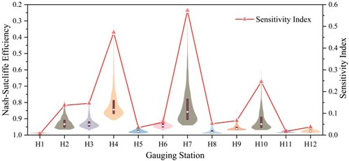
Figure 5 shows the spatial distribution of the SI in the study area. It was drawn by the kriging method with the calculated SI of each point in the model. The sensitivity is strongest in the central region of the study area but weaker in the northern and southern areas. The model structure and boundary conditions can be used to explain this spatial difference. Some studies indicated that boundary conditions strongly impact the measured data of gauging stations close to the boundary conditions (Dung et al., 2010; Jahandideh-Tehrani et al., 2020; Yang et al., 2014). The weakest sensitivity region can be found in the north of the study area close to the water boundary. In addition, the regions around gauging stations H11 and H5 show weaker sensitivity. In fact, the ground elevation of these regions is relatively low. Therefore, pumps inside these regions were operated to prevent higher water levels for safety during the experiment. Thus far, the boundary conditions and operation state of water conservancy projects have been found to greatly impact the sensitivity of the internal water level in the plain river network area. The operation of the pumping stations on the southern boundary can account for the slightly weaker sensitivity in the southern region. In turn, the large difference in the spatial distribution of the SI illustrates the importance of identifying the weights of multiple stations.

Figure 5. Spatial distribution of SI in study area as drawn using a kriging method with the calculated SI of each point in the simulation model.

3.2. Calibration performance

For the PSO algorithm, the particle population and maximum iterations were set to 20 and 400, respectively. Therefore, the total number of realizations of the optimization-simulation model was 8000. The simulation of each realization took ∼5 s, and the whole calibration process took ∼12 h. The calibration performance is illustrated through visual inspections and evaluation criteria. For the global performance, Figure 6 describes the relationship between the simulation numbers and the objective function fitness. The simulation fitness decreased with an increase in the number of simulations. The maximization of this range was 0.2 at the beginning of the simulation (1st generation), and this range of fitness values for each particle reduced to 0.004 after 300 simulations (15th generation). Additionally, the global best fitness varied from 0.926 to 0.95. When the simulation number was increased to 2000, the global optimal fitness almost became stable. The results showed that the PSO algorithm has a high global search performance. In this algorithm, the movement of each individual is attracted by the previous promising position and best position of the population simultaneously. In other words, this algorithm combines individual self-learning and group learning characteristics that can help to find the optimal solution with fewer iterations.

Figure 6. Gray line with blue triangles indicates fitness of each simulation. Each generation has 20 particles (realizations). Red line indicates global best fitness of each generation.

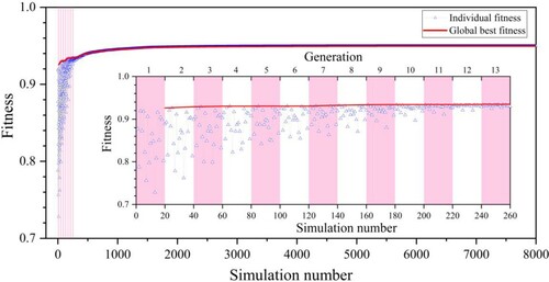
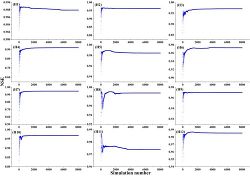
Figure 7 shows, the NSE of each station during the model calibration. A certain difference is seen in the NSE of each station. With an increasing number of simulations, the NSE keeps increasing until it becomes stable for most gauging stations (8 out of 12), indicating that the optimal global fitness is obtained. Some sacrifice in NSE is seen for H1, H5, H11, and H12. The best NSE for these stations is not achieved in the last simulation. The sacrifice of these stations is to obtain the optimal global fitness based on the objective function indicated previously.

Figure 7. Individual performance during calibration. Blue triangles indicate NSE of each station for each simulation.

To measure the individual performance for each gauging station, NSE, R, and PBIAS were used. Table 4 lists all criteria results. NSE ranged from 0.898 to 0.99, R ranged from 0.95 to 0.995, and PBIAS ranged from −2.08 to 0.37. Figure 8 shows the calibration results of the 12 gauging stations. The best simulation and observed data are indicated by the red line and blue triangles, respectively. The best simulated water level is in good agreement with the observed data for each station. The calculation results and efficiency indicate that the proposed method has high model calibration performance.

Figure 8. Calibration results for gauging stations. Red lines indicate best simulation results, and blue triangles indicate observed data.

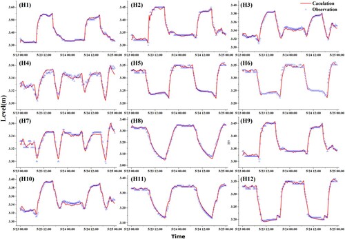
Table 4. Performance of optimization-simulation model for each gauging station. NSE, R, and PBIAS are shown for the best simulation.

	Gauging station
Criteria	H1	H2	H3	H4	H5	H6	H7	H8	H9	H10	H11	H12
NSE	0.990	0.966	0.964	0.898	0.983	0.975	0.935	0.989	0.973	0.963	0.978	0.985
R	0.995	0.983	0.982	0.950	0.993	0.988	0.967	0.995	0.987	0.982	0.994	0.993
PBIAS	0.35	−0.14	0.07	0.05	−0.78	−0.23	0.03	0.37	−0.22	0.03	−2.08	−0.42

3.3. Calibrated parameter values

Figure 9 shows the spatial distribution of the ‘optimal’ Manning’s roughness coefficients. The roughness distributions in Figure 9 indicate that the roughness coefficients of most major river reaches are small (89.3% along length of major river reaches) and those of minor river reaches are comparatively larger (81.1% along length of minor river reaches). This tendency is consistent with reality, and it indicates that the roughness set determined by model calibration is reasonable.

Figure 9. Spatial distribution of optimal Manning roughness coefficients as estimated using optimization-simulation model. Some river reaches with unreasonable roughness are marked by a red dotted line.

However, the roughness of some river reaches is slightly irrational. For example, a few minor river reaches with smaller roughness are seen in Figure 9. In addition, some major river reaches (indicated by red dotted line) have larger roughness. There are three possible reasons for these unreasonable results.

1. They are affected by boundary conditions. This was seen in the first circle of rivers that were close to the water boundary and that had weaker sensitivity (Figure 5).

2. They are affected by the operation of pumps and sluices. The n values of the major river reaches in the second circle are relatively smaller. These river reaches have lower velocity because the sluice structure to the east of the major rivers was maintained during the experiment.

3. They compensate for the sources of errors (Fabio et al., 2010; Kouchi et al., 2017). The balance of all types of errors in the model is another important reason for the unreasonable roughness. These findings show that the estimation of the roughness structure of a complex plain river network can be affected by the boundary conditions and operation of the pumping stations and sluice structures. In future calibration, various data sources, including not only water level data but also flow data, need to be considered. Compared with water level data, flow data often have low accuracy and lower data frequency owing to measurement-related reasons. Therefore, the application of these two different data sources with different precision and data frequencies in roughness calibration is worth studying further. In general, the roughness of all river reaches in the study area can be easily acquired by the high-efficiency and -accuracy optimization-simulation method.

4. Conclusions

The results of this study can be summarized as follows:

1. A coupled optimization-simulation model was proposed to systematically estimate the spatial distribution of n values with river reaches in a plain looped river network area. The PSO algorithm and InfoWorks ICM software were integrated to solve the objective function and hydraulic process, respectively. The results showed that the PSO algorithm has high global search performance, and the proposed approach performs well in identifying the optimal Manning’s roughness coefficients in the plain river network area.

2. Unlike in most previous studies, crisscrossing rivers were partitioned into river reaches where each reach was assumed to have a uniform and constant Manning’s roughness coefficient according to its network topology and cross-section variation. This method can balance the accuracy and calibration workloads in a complicated river network.

3. A sensitivity analysis was implemented to determine the weights of measured data from different gauging stations. The sensitivity analysis results revealed that the boundary conditions and the operation state of water conservancy projects greatly impact the internal water level. The large difference in the spatial distribution of the SI also illustrated the importance of identifying the weights of multiple stations.

4. Generally, the spatial distribution of optimal Manning’s roughness coefficients was consistent with the reality. The roughness coefficients of most major river reaches were small (89.3% along length of major river reaches), and those of minor river reaches were comparatively larger (81.1% along length of minor river reaches). The n values of some river reaches were slightly irrational owing to the compensation of error sources, influence of boundary conditions, and operation of pumps and sluices.

Although this study provides insights for estimating the spatial distribution of Manning’s roughness coefficients in plain looped river network areas, some issues require further consideration. In future studies, various data sources, such as water level data and flow data, could be considered for model calibration. In addition, the uncertainty of data sources and the equifinality of accepted roughness sets could be analyzed in detail. Furthermore, the influence of different optimization algorithm parameters on the solution accuracy could be analyzed.

Acknowledgments

This work was supported by the National Key Research and Development Program of China under Grant [2018YFC0407205]; and the China Postdoctoral Science Foundation under Grant [2019M661884]. We thank Yingjian Xu from Changshu Water Bureau for providing basic data. We also sincerely thank the reviewers who contributed their expertise and time on reviewing this manuscript. Conceptualization, Fan Yang and Ziwu Fan; Methodology, Fan Yang, Jingxiu Wu; Project administration, Ziwu Fan; Investigation, Guoqing Liu and Guangyu Chen; Writing – original draft, Fan Yang; Writing – review & editing, Fan Yang, Senlin Zhu, Shiqiang Wu and Jingxiu Wu.

Disclosure statement

No potential conflict of interest was reported by the author(s).

Additional information

Funding

This work was supported by the National Key Research and Development Program of China under grant: [grant number 2018YFC0407205]; and the China Postdoctoral Science Foundation under Grant [2019M661884].

References

- Andréassian, V., Perrin, C., Berthet, L., Le Moine, N., Lerat, J., Loumagne, C., Oudin, L., Mathevet, T., Ramos, M. H., & Valéry, A. (2009). HESS opinions “Crash tests for a standardized evaluation of hydrological models”. Hydrology and Earth System Sciences, 13(10), 1757–1764. https://doi.org/https://doi.org/10.5194/hess-13-1757-2009
- Arcement, G. J., & Schneider, V. R. (1989). Guide for selecting Manning's roughness coefficients for natural channels and flood plains.
- Attari, M., & Hosseini, S. M. (2019). A simple innovative method for calibration of Manning’s roughness coefficient in rivers using a similarity concept. Journal of Hydrology, 575, 810–823. https://doi.org/https://doi.org/10.1016/j.jhydrol.2019.05.083
- Ayvaz, M. T. (2013). A linked simulation–optimization model for simultaneously estimating the Manning’s surface roughness values and their parameter structures in shallow water flows. Journal of Hydrology, 500, 183–199. https://doi.org/https://doi.org/10.1016/j.jhydrol.2013.07.019
- Ayvaz, M. T., & Genç, Ö. (2012). Optimal estimation of Manning’s roughness in open channel flows using a Linked simulation-optimization model. BALWOIS.
- Bajpai, P., & Singh, S. N. (2007). Fuzzy adaptive particle swarm optimization for bidding strategy in uniform price spot market. IEEE Transactions on Power Systems, 22(4), 2152–2160. https://doi.org/https://doi.org/10.1109/tpwrs.2007.907445
- Barnes, H. H. (1967). Roughness characteristics of natural channels. US Government Printing Office.
- Bekele, E. G., & Nicklow, J. W. (2007). Multi-objective automatic calibration of SWAT using NSGA-II. Journal of Hydrology, 341(3-4), 165–176. https://doi.org/https://doi.org/10.1016/j.jhydrol.2007.05.014
- Boulomytis, V. T. G., Zuffo, A. C., Dalfré Filho, J. G., & Imteaz, M. A. (2017). Estimation and calibration of Manning’s roughness coefficients for ungauged watersheds on coastal floodplains. International Journal of River Basin Management, 15(2), 199–206. https://doi.org/https://doi.org/10.1080/15715124.2017.1298605
- Brighenti, T. M., Bonumá, N. B., Grison, F., Mota, A. A., Kobiyama, M., & Chaffe, P. L. B. (2019). Two calibration methods for modeling streamflow and suspended sediment with the swat model. Ecological Engineering, 127, 103–113. https://doi.org/https://doi.org/10.1016/j.ecoleng.2018.11.007
- Choo, Y. M., Yun, G. S., & Choo, T. H. (2018). A research on the estimation of coefficient roughness in open channel applying entropy concept. Environmental Earth Sciences, 77(17). https://doi.org/https://doi.org/10.1007/s12665-018-7809-4
- Chow, V. T. (1959). Open-channel hydraulics. McGraw-Hill.
- Chow, V. T. (1988). Applied hydrology. Tata McGraw-Hill Education.
- Cowan, W. L. (1956). Estimating hydraulic roughness coefficients. Agricultural Engineering, 37(7), 473–475.
- De Doncker, L., Troch, P., Verhoeven, R., Bal, K., Meire, P., & Quintelier, J. (2009). Determination of the Manning roughness coefficient influenced by vegetation in the river Aa and Biebrza river. Environmental Fluid Mechanics, 9(5), 549–567. https://doi.org/https://doi.org/10.1007/s10652-009-9149-0
- Ding, Y., Jia, Y., & Wang, S. S. Y. (2004). Identification of Manning’s roughness coefficients in shallow water flows. Journal of Hydraulic Engineering, 130(6), 501–510. https://doi.org/https://doi.org/10.1061/(asce)0733-9429(2004)130:6(501)
- Ding, Y., & Wang, S. S. Y. (2005). Identification of Manning's roughness coefficients in channel network using adjoint analysis. International Journal of Computational Fluid Dynamics, 19(1), 3–13. https://doi.org/https://doi.org/10.1080/10618560410001710496
- Duan, Q. Y., Gupta, V. K., & Sorooshian, S. (1993). Shuffled complex evolution approach for effective and efficient global minimization. Journal of Optimization Theory and Applications, 76(3), 501–521. https://doi.org/https://doi.org/10.1007/bf00939380
- Dung, N. V., Merz, B., Bárdossy, A., Thang, T. D., & Apel, H. (2010). Multi-objective automatic calibration of hydrodynamic models utilizing inundation maps and gauge data. Hydrology and Earth System Sciences Discussions, 7(6), 9173–9218. https://doi.org/https://doi.org/10.5194/hessd-7-9173-2010
- Efstratiadis, A., & Koutsoyiannis, D. (2010). One decade of multi-objective calibration approaches in hydrological modelling: A review. Hydrological Sciences Journal, 55(1), 58–78. https://doi.org/https://doi.org/10.1080/02626660903526292
- Fabio, P., Aronica, G. T., & Apel, H. (2010). Towards automatic calibration of 2-D flood propagation models. Hydrology and Earth System Sciences, 14(6), 911–924. https://doi.org/https://doi.org/10.5194/hess-14-911-2010
- Fong, S., Wong, R., & Vasilakos, A. (2015). Accelerated PSO swarm search feature selection for data stream mining big data. IEEE Transactions on Services Computing, 9(1), 1–1. https://doi.org/https://doi.org/10.1109/tsc.2015.2439695
- Fotovatikhah, F., Herrera, M., Shamshirband, S., Chau, K.-w., Faizollahzadeh Ardabili, S., & Piran, M. J. (2018). Survey of computational intelligence as basis to big flood management: Challenges, research directions and future work. Engineering Applications of Computational Fluid Mechanics, 12(1), 411–437. https://doi.org/https://doi.org/10.1080/19942060.2018.1448896
- Foulon, É, & Rousseau, A. N. (2018). Equifinality and automatic calibration: What is the impact of hypothesizing an optimal parameter set on modelled hydrological processes? Canadian Water Resources Journal / Revue Canadienne des Ressources Hydriques, 43(1), 47–67. https://doi.org/https://doi.org/10.1080/07011784.2018.1430620
- Gholami, A., Bonakdari, H., Zaji, A. H., Ajeel Fenjan, S., & Akhtari, A. A. (2016). Design of modified structure multi-layer perceptron networks based on decision trees for the prediction of flow parameters in 90° open-channel bends. Engineering Applications of Computational Fluid Mechanics, 10(1), 193–208. https://doi.org/https://doi.org/10.1080/19942060.2015.1128358
- Gupta, H. V., Sorooshian, S., & Yapo, P. O. (1998). Toward improved calibration of hydrologic models: Multiple and noncommensurable measures of information. Water Resources Research, 34(4), 751–763. https://doi.org/https://doi.org/10.1029/97wr03495
- Gupta, H. V., Sorooshian, S., & Yapo, P. O. (1999). Status of automatic calibration for hydrologic models: comparison with multilevel expert calibration. Journal of Hydrologic Engineering, 4(2), 135–143. https://doi.org/https://doi.org/10.1061/(asce)1084-0699(1999)4:2(135)
- Hadiyanto, H., Elmore, S., Van Gerven, T., & Stankiewicz, A. (2013). Hydrodynamic evaluations in high rate algae pond (HRAP) design. Chemical Engineering Journal, 217, 231–239. https://doi.org/https://doi.org/10.1016/j.cej.2012.12.015
- Hameed, L. K., & Ali, S. T. (2013). Estimating of Manning’s roughness coefficient for Hilla River through calibration using HEC-RAS model. Jordan Journal of Civil Engineering, 7(1), 44–53.
- Her, Y., & Seong, C. (2018). Responses of hydrological model equifinality, uncertainty, and performance to multi-objective parameter calibration. Journal of Hydroinformatics, 20(4), 864–885. https://doi.org/https://doi.org/10.2166/hydro.2018.108
- Holden, N., & Freitas, A. A. (2008). A hybrid PSO/ACO algorithm for discovering classification rules in data mining. Journal of Artificial Evolution and Applications, 2008, 1–11. https://doi.org/https://doi.org/10.1155/2008/316145
- Huang, X., & Xiang, L. (2017). Field prototype experiment of water diversion for river network in south of Changshu city (In Chinese). Water Resources and Power, 35, 69–72.
- Jahandideh-Tehrani, M., Helfer, F., Zhang, H., Jenkins, G., & Yu, Y. (2020). Hydrodynamic modelling of a flood-prone tidal river using the 1D model MIKE HYDRO River: Calibration and sensitivity analysis. Environmental Monitoring and Assessment, 192(2), 97. https://doi.org/https://doi.org/10.1007/s10661-019-8049-0
- Jiang, L., Wu, H., Tao, J., Kimball, J. S., Alfieri, L., & Chen, X. (2020). Satellite-based evapotranspiration in hydrological model calibration. Remote Sensing, 12(3), 428. https://doi.org/https://doi.org/10.3390/rs12030428
- Kennedy, J., & Eberhart, R. (1995). Particle swarm optimization. Proceedings of ICNN'95-International Conference on Neural Networks.
- Kirchner, J. W. (2006). Getting the right answers for the right reasons: Linking measurements, analyses, and models to advance the science of hydrology. Water Resources Research, 42(3). https://doi.org/https://doi.org/10.1029/2005wr004362
- Kouchi, D. H., Esmaili, K., Faridhosseini, A., Sanaeinejad, S. H., Khalili, D., & Abbaspour, K. C. (2017). Sensitivity of calibrated parameters and water resource estimates on different objective functions and optimization algorithms. Water, 9(6), 384. https://doi.org/https://doi.org/10.3390/w9060384
- Kurnatowski, J. (2013). Inverse problem for looped river networks – lower oder river case study. Archives of Environmental Protection, 39(1), 105–118. https://doi.org/https://doi.org/10.2478/aep-2013-0010
- Lacasta, A., Morales-Hernández, M., Burguete, J., Brufau, P., & García-Navarro, P. (2017). Calibration of the 1D shallow water equations: A comparison of Monte Carlo and gradient-based optimization methods. Journal of Hydroinformatics, 19(2), 282–298. https://doi.org/https://doi.org/10.2166/hydro.2017.021
- Li, L., Xue, B., Niu, B., Chai, Y., & Wu, J. (2009). The novel non-linear strategy of inertia weight in particle swarm optimization. 2009 Fourth International on Conference on Bio-Inspired Computing.
- Li, Z., & Zhang, J. (2001). Calculation of field Manning’s roughness coefficient. Agricultural Water Management, 49(2), 153–161. https://doi.org/https://doi.org/10.1016/s0378-3774(00)00139-6
- Madsen, H. (2003). Parameter estimation in distributed hydrological catchment modelling using automatic calibration with multiple objectives. Advances in Water Resources, 26(2), 205–216. https://doi.org/https://doi.org/10.1016/s0309-1708(02)00092-1
- Malaterre, O., Baume, J.-P., Jean-Baptiste, N., & Sau, J. (2010). Calibration of open channel flow models: a system analysis and control engineering approach. SimHydro 2010: Hydraulic modeling and uncertainty, Sophia-Antipolis, France.
- McKay, M. D., Beckman, R. J., & Conover, W. J. (1979). Comparison of three methods for selecting values of input variables in the analysis of output from a computer code. Technometrics, 21(2), 239–245. https://doi.org/https://doi.org/10.1080/00401706.1979.10489755
- Nash, J. E., & Sutcliffe, J. V. (1970). River flow forecasting through conceptual models part I — A discussion of principles. Journal of Hydrology, 10(3), 282–290. https://doi.org/https://doi.org/10.1016/0022-1694(70)90255-6
- Neumayer, M., Teschemacher, S., Schloemer, S., Zahner, V., & Rieger, W. (2020). Hydraulic modeling of Beaver Dams and evaluation of their impacts on flood events. Water, 12(1), 300. https://doi.org/https://doi.org/10.3390/w12010300
- Ong, T. D. B., Doscher, C., & Mohssen, M. (2017). Simulated annealing for calibrating the Manning’s roughness coefficients for general channel networks on a basin scale. Arabian Journal of Geosciences, 10(24). https://doi.org/https://doi.org/10.1007/s12517-017-3320-6
- Orlandini, S. (2002). On the spatial variation of resistance to flow in upland channel networks. Water Resources Research, 38(10), 15-1–15-14. https://doi.org/https://doi.org/10.1029/2001wr001187
- Ozcan, E., & Mohan, C. K. (1999). Particle swarm optimization: surfing the waves. Proceedings of the 1999 Congress on Evolutionary Computation-CEC99.
- Parhi, P. K., Sankhua, R. N., & Roy, G. P. (2012). Calibration of channel roughness for Mahanadi River, (India) using HEC-RAS model. Journal of Water Resource and Protection, 04(10), 847–850. https://doi.org/https://doi.org/10.4236/jwarp.2012.410098
- Pasternack, G. B., Wang, C. L., & Merz, J. E. (2004). Application of a 2D hydrodynamic model to design of reach-scale spawning gravel replenishment on the Mokelumne River, California. River Research and Applications, 20(2), 205–225. https://doi.org/https://doi.org/10.1002/rra.748
- Peng, H., Liu, Y., Wang, H., Gao, X., Chen, Y., & Ma, L. (2016). Urban stormwater forecasting model and drainage optimization based on water environmental capacity. Environmental Earth Sciences, 75(14), 1094. https://doi.org/https://doi.org/10.1007/s12665-016-5824-x
- Peng, H. Q., Liu, Y., Wang, H. W., & Ma, L. M. (2015). Assessment of the service performance of drainage system and transformation of pipeline network based on urban combined sewer system model. Environmental Science and Pollution Research, 22(20), 15712–15721. https://doi.org/https://doi.org/10.1007/s11356-015-4707-0
- Ramesh, R., Datta, B., Bhallamudi, S. M., & Narayana, A. (2000). Optimal estimation of roughness in open-channel flows. Journal of Hydraulic Engineering, 126(4), 299–303. https://doi.org/https://doi.org/10.1061/(asce)0733-9429(2000)126:4(299)
- Rezaee Jordehi, A., & Jasni, J. (2013). Parameter selection in particle swarm optimisation: A survey. Journal of Experimental & Theoretical Artificial Intelligence, 25(4), 527–542. https://doi.org/https://doi.org/10.1080/0952813x.2013.782348
- Sengupta, S., Basak, S., & Peters, R. (2018). Particle swarm optimization: A survey of historical and recent developments with hybridization perspectives. Machine Learning and Knowledge Extraction, 1(1), 157–191. https://doi.org/https://doi.org/10.3390/make1010010
- Shamshirband, S., Jafari Nodoushan, E., Adolf, J. E., Abdul Manaf, A., Mosavi, A., & Chau, K.-w. (2018). Ensemble models with uncertainty analysis for multi-day ahead forecasting of chlorophyll a concentration in coastal waters. Engineering Applications of Computational Fluid Mechanics, 13(1), 91–101. https://doi.org/https://doi.org/10.1080/19942060.2018.1553742
- Shi, Y., & Eberhart, R. C. (1998). Parameter selection in particle swarm optimization. International conference on evolutionary programming.
- Shi, Y., & Eberhart, R. C. (1999). Empirical study of particle swarm optimization. Proceedings of the 1999 congress on evolutionary computation-CEC99 (Cat. No. 99TH8406).
- Tayfur, G., Singh, V., Moramarco, T., & Barbetta, S. (2018). Flood hydrograph prediction using machine learning methods. Water, 10(8), 968. https://doi.org/https://doi.org/10.3390/w10080968
- Timbadiya, P. V., Patel, P. L., & Porey, P. D. (2011). Calibration of HEC-RAS model on prediction of flood for lower Tapi River, India. Journal of Water Resource and Protection, 03(11), 805–811. https://doi.org/https://doi.org/10.4236/jwarp.2011.311090
- Van der Merwe, D., & Engelbrecht, A. P. (2003). Data clustering using particle swarm optimization. The 2003 Congress on Evolutionary Computation, 2003. CEC'03.
- van Griensven, A., Meixner, T., Grunwald, S., Bishop, T., Diluzio, M., & Srinivasan, R. (2006). A global sensitivity analysis tool for the parameters of multi-variable catchment models. Journal of Hydrology, 324(1-4), 10–23. https://doi.org/https://doi.org/10.1016/j.jhydrol.2005.09.008
- Wang, H., Lei, X., Khu, S.-T., & Song, L. (2019). Optimization of pump start-up depth in drainage pumping station based on SWMM and PSO. Water, 11(5), 1002. https://doi.org/https://doi.org/10.3390/w11051002
- Yang, T.-H., Wang, Y.-C., Tsung, S.-C., & Guo, W.-D. (2014). Applying micro-genetic algorithm in the one-dimensional unsteady hydraulic model for parameter optimization. Journal of Hydroinformatics, 16(4), 772–783. https://doi.org/https://doi.org/10.2166/hydro.2013.030
- Yao, S., Guo, D., Sun, Z., & Yang, G. (2015). A modified multi-objective sorting particle swarm optimization and its application to the design of the nose shape of a high-speed train. Engineering Applications of Computational Fluid Mechanics, 9(1), 513–527. https://doi.org/https://doi.org/10.1080/19942060.2015.1061557
- Yapo, P. O., Gupta, H. V., & Sorooshian, S. (1996). Automatic calibration of conceptual rainfall-runoff models: Sensitivity to calibration data. Journal of Hydrology, 181(1-4), 23–48. https://doi.org/https://doi.org/10.1016/0022-1694(95)02918-4
- Yen, B. C. (1973). Open-channel flow equations revisited. Journal of the Engineering Mechanics Division, 99(5), 979–1009.
- Zeng, N., Zhang, H., Liu, W., Liang, J., & Alsaadi, F. E. (2017). A switching delayed PSO optimized extreme learning machine for short-term load forecasting. Neurocomputing, 240, 175–182. https://doi.org/https://doi.org/10.1016/j.neucom.2017.01.090