MAST-RT0 solution of the incompressible Navier–Stokes equations in 3D complex domains

Abstract

A new numerical methodology to solve the 3D Navier-Stokes equations for incompressible fluids within complex boundaries and unstructured body-fitted tetrahedral mesh is presented and validated with three literature and one real-case tests. We apply a fractional time step procedure where a predictor and a corrector problem are sequentially solved. The predictor step is solved applying the MAST (Marching in Space and Time) procedure, which explicitly handles the non-linear terms in the momentum equations, allowing numerical stability for Courant number greater than one. Correction steps are solved by a Mixed Hybrid Finite Elements discretization that assumes positive distances among tetrahedrons circumcentres. In 3D problems, non-Delaunay meshes are provided by most of the mesh generators. To maintain good matrix properties for non-Delaunay meshes, a continuity equation is integrated over each tetrahedron, but the momentum equations are integrated over clusters of tetrahedrons, such that each external face shared by two clusters belongs to two tetrahedrons whose circumcentres have positive distance. A numerical procedure is proposed to compute the velocities inside clusters with more than one tetrahedron. Model preserves mass balance at the machine error and there is no need to compute pressure at each time iteration, but only at target simulation times.

KEYWORDS:

• Navier–Stokes equations
• 3D numerical model
• Eulerian method
• unstructured tetrahedral mesh
• predictor–corrector scheme
• Mixed Hybrid Finite element

1. Introduction

The Navier–Stokes Equations (NSEs) govern external and internal flows in many real-life industrial, environmental and biological problems (e.g. aircraft and ship problems, rotomachinery blade applications, hemodynamic and biological flows). The challenging research topics involved in the numerical solution of such mathematical problems mainly concern the choice of the velocity-pressure coupling algorithm and the design of the computational mesh discretizing the physical domain.

In compressible flows, pressure and density are linked by the state algebraic equation. In contrast, in incompressible flows, density is constant and pressure has to be solved along with velocities from all the momentum and continuity equations. With this motivation, the numerical algorithms used to solve the NSEs can generally be divided into density-based and pressure-based solvers (Shyy & Mittal, 1998; Tao, 2001). Density-based solvers are commonly applied to high-Ma compressible flows, while pressure-based solvers were originally proposed for incompressible flows, and then successfully extended to compressible flows (Tao, 2001).

Two approaches are generally used in pressure-based solvers, namely the direct (or coupled) approach and the segregated approach (e.g. Mazhar, 2016 and cited references). In the first case, the whole set of momentum and continuity equations is solved simultaneously, resulting in a strong coupling between pressure and velocity. The main drawback is the large amount of required computational effort and computer memory, which makes this approach unsuitable to facing many practical engineering applications (Darwish et al., 2015). In the segregated approach, pressure and velocity are solved separately and sequentially, using previously computed values of the other dependent variable. The core of the problem is how to update the pressure field so that the divergence-free velocity field condition is satisfied.

Several numerical procedures can be distinguished in the segregated approach, e.g. the projection method (Chorin, 1968; Kim & Moin, 1985), the penalty method (Braaten & Shyy, 1986; Hughes et al., 1979), the artificial compressibility method (Harlow & Welch, 1965; Malan et al., 2002; Vrahliotis et al., 2012), and the pressure-correction method (Ozoe & Tao, 2001; Patankar, 1980).

The fractional step projection method (Chorin, 1968; Kim & Moin, 1985) and the SIMPLE (Semi-Implicit Method for Pressure-Linked Equations) pressure-correction method (Patankar, 1980, 1981) have become very popular. In both methodologies, a pressure correction is introduced to improve the velocities computed from the solution of the momentum equations, and to satisfy the continuity equation. Projection methods, commonly regarded as fractional-step methods, can be classified into pressure-correction methods, velocity-correction methods and consistent splitting methods (Guermond et al., 2006). A sequence of decoupled elliptic equations for velocity and pressure has to be solved at each time step, and this represents one of the most attractive features of such procedures, especially for simulations of large-scale problems (Guermond et al., 2006). In the projection method, the pressure correction Poisson equation is solved once per time step, while for the SIMPLE method, the momentum and pressure correction equations are solved several times in each time step. For these reasons, projection methods could handle unsteady flow problems more easily than SIMPLE.

The SIMPLE-family algorithms (e.g. SIMPLER, SIMPLEC, SIMPLEX) are extensions of and improvements to the SIMPLE algorithm. Other pressure correction methods can be regarded as further extensions of the SIMPLE-family models, for example PISO and CLEAR (e.g. Aguerre et al., 2020 and cited works). Segregated solvers like the SIMPLE-family algorithms have shown poor convergence, especially when used for swirling flow fields (Hanby & Silvester, 1996). In these problems, where the coupling between radial and tangential momentum equations is strong, the linearization of the momentum equations leads to a sequential solution of these equations, without accounting for the coupling between the momentum equations and the velocity components (Hanby & Silvester, 1996). Even though several ‘ad hoc’ procedures have been presented in order to overcome the above-mentioned convergence problems (e.g. Gosman et al., 1976), the need of parameter calibration for convergence of the iterative procedure requires a high computational effort, which limits the application of these algorithms. These reasons, along with the increase of computer performance and memory, have motivated several authors towards new coupled approaches (e.g. Darwish et al., 2009 and cited references).

Other options have been proposed in the literature, e.g. the vorticity-stream function methods, where pressure is eliminated from the governing equations and velocity and pressure are replaced by the vorticity and the stream function (e.g. Calhoun, 2002 and cited references). Two main reasons have limited their use: the difficulty of handling wall boundary conditions and the difficulties arising in the extension from 2D to 3D problems (Calhoun, 2002).

It is widely recognized that spatial discretization of the incompressible flow equations on collocated grids leads to unphysical odd–even coupling of the pressure (i.e. the so-called spurious checkerboard modes) (e.g. Dalal et al., 2008; Perron et al., 2004). Staggered grids have been one of the most common ways to overcome these problems, where different grid points for velocity and pressure are used (e.g. Harlow & Welch, 1965; Perot, 2000).

In the last decade, the use of unstructured grids has become popular due to their capacity to discretize real arbitrary domains and to easily get local refinement. Geometric complexity is a drawback for a straightforward extension of the staggered mesh to unstructured grids and most solvers require the addition of terms which could generate unphysical solutions and loss of mass conservations (e.g. Perot, 2000). Moreover, the time step limitation required by the Courant condition can become very severe, due to the existence of few computational elements much smaller than the average ones.

In the past few decades, Finite Volume Methods (FVMs) (e.g. Kim & Choi, 2000; Mathur & Murthy, 1997; Perron et al., 2004; Plana Fattori et al., 2013; Vidovic et al., 2004) and Finite Element Methods (FEMs) (e.g. Bazilevs et al., 2013; Fortin, 1981; Pai et al., 2013; Zienkiewicz et al., 2013) have been preferred to other methods (e.g. finite difference methods) in handling irregular boundaries, because they can use unstructured triangular or tetrahedral meshes, which can easily discretize arbitrary geometries. A large multitude of FVMs has been proposed in the last few decades, with different choices of control volumes, both for collocated and staggered grids. Many of these proposed techniques suffer from a ‘non-orthogonality condition’, as pointed out in (Gao et al., 2012), in discretization of the second-order partial derivative terms in the momentum equations and in the pressure-correction Poisson equation. Hybrid FV/FEMs (e.g. Busto et al., 2018; Gao et al., 2012) take advantage of both FVMs and FEMs, discretizing the momentum equations with the FVMs and the Poisson equation with the FEMs. The Discontinuous Galerkin Finite Element Methods (DG-FEMs) (e.g. Bassi & Rebay, 1997; Lehrenfeld & Schöberl, 2016 and cited references) combine the performing features of the FEMs and FVMs. Like the classical FEMs, the DG-FEMs achieve high-order accuracy using high-order polynomial approximation within an element rather than using wide stencils, as in the case of finite volume methods. The physics of wave propagation is however correctly accounted for by the solution of a Riemann problem (e.g. Toro et al., 2020 and cited references) arising from the discontinuous solution at element interfaces, which makes them similar to FVMs (e.g. Toro & Vazquez-Cendon, 2012). The main drawback of DG-FEMs, compared to the classical FEMs and FVMs, is that they require solutions of systems of equations with more unknowns for the same grids, and have been recognized to be very demanding in terms of both computational costs and storage requirements.

Recently, mesh-free methods have received increasing attention from researchers, due to their ability to solve flow problems with complex geometries or involving multi-phases fluids. The Smoothed Particle Hydrodynamics (SPH) method is a pure Lagrangian, mesh-free procedure, originally proposed for the solution of astrophysical problems (Gingold & Monaghan, 1977; Lucy, 1977). The fluid domain is discretized by a set of moving particles, and the governing equations are solved for each of them. Each particle has a support domain with a characteristic spatial distance over which their physical properties (namely pressure and velocity) are ‘smoothed’ by means of a kernel function, generally with a Gaussian-type shape. Thanks to its quite easy implementation, this procedure has largely been applied for the solution of compressible and incompressible NSEs (e.g. Oger et al., 2007 and cited references). One of the main drawbacks of the Lagrangian schemes is that the relations among particles have to be updated at each time step, and the topology setting of the matrix system of the Poisson pressure-correction equations has to be performed at each time iteration, as well as its factorization operations.

During the last years, Virtual Elements Methods (VEMs) (e.g. Beirão da Veiga et al., 2018, and cited references) have been proposed as a new FEM paradigm to solve Partial Differential Equations. VEMs construct a conforming Galerkin FE scheme, dealing with general polygonal/polyhedral mesh elements, also with non-convex shape. VEMs have been recently applied for the solution of the NSEs in 2D problems (e.g. Beirão da Veiga et al., 2018, and cited references), but their extension to 3D problems is still limited to very simple domain geometries and boundary shapes (Liu & Chen, 2019).

In the present paper, we propose a new finite volume solver for the solution of 3D incompressible NSEs over unstructured tetrahedral meshes. We apply a fractional time step procedure where a predictor and a corrector problem are sequentially solved. The procedure presents substantial differences compared to the fractional step procedures presented in the literature, based upon the common projection procedures (e.g. Guermond et al., 2006; Perron et al., 2004). The predictor step (PS) is carried out by applying the Eulerian Finite Volume MAST (Marching in Space and Time) numerical procedure, recently proposed for the solution of shallow waters and groundwater problems (Aricò et al., 2007; Aricò et al., 2011, 2012, 2013a, 2013b; Aricò & Tucciarelli, 2007a, 2007b, 2009). In this step, all the terms are retained in the momentum equations. The major advantages of MAST are the following: (1) it explicitly handles the non-linear momentum terms in the momentum equations, by means of the sequential solution of a three-variable Ordinary Differential Equations (ODEs) system for each computational cell, with a computational effort which is simply proportional to the number of tetrahedral elements, (2) it provides numerical stability with respect to large Courant–Friedrichs-Lewy (CFL) numbers, that can be much greater than one, at a cost of local accuracy reduction (Aricò et al., 2007; Aricò & Tucciarelli, 2007a, 2007b). The correction step is split into two parts, named CS1 step and CS2 step. In CS1 step, three linear systems are solved for the three velocity components (one system for each velocity component), which update the viscous terms in the momentum equations. In the second corrector step (CS2), a single linear system is solved for the pressure correction unknown. The matrices of the systems of CS1 and CS2 steps are well conditioned, as they are sparse, symmetric and diagonally dominant, and lead to a very fast solution of the associated systems by the use of a preconditioned conjugated gradient solver. The matrix coefficients are constant in time, computed and factorized only once at the beginning of the numerical simulation. This makes it possible to save a lot of computational time, compared to other numerical schemes (e.g. Lagrangian schemes).

Both CS1 and CS2 steps are solved assuming a mass lumping Mixed Hybrid Finite Element (MHFE) (e.g. Auricchio et al., 2017, and cited references) discretization inside each tetrahedron, similar to the one proposed by Younes et al. (2006). The mass lumping option has been chosen because it is easy to be used together with tetrahedral elements. To maintain good convergence and accuracy properties, our MHFE scheme assumes the distance among circumcenters to be positive, a condition which is always satisfied in the Delaunay meshes. Unfortunately, in 3D problems either bad-quality Delaunay or non-Delaunay meshes are provided by most of the available mesh generators (Li & Teng, 2001). To cope with this problem, and to use non-Delaunay meshes still saving the previously mentioned good matrix properties, in the present procedure, a continuity equation is integrated over each single tetrahedron, but the momentum equations are integrated over clusters of tetrahedrons, such that each external face shared by two different clusters is part of two tetrahedrons whose circumcenters have positive distance. To define the velocities inside each cluster with more than one tetrahedron correctly, the minimum energy condition is finally enforced for velocities inside the clusters.

In the proposed numerical solver, mass balance is always preserved at the error machine precision, and there is no need to update the pressure values at each time iteration, because only the pressure gradient appear in the NSEs. We compute the spatial pressure distribution only at target simulation times.

The paper is organized as follows. In section 2.1, we present the governing equations and the projection-correction formulation of the problem and in section 2.2 the spatial discretization. In sections 3.1, 3.2, and 3.3, we present the numerical details of the solution of respectively the PS, CS1 and CS2 steps as defined in section 2.1. In section 4, we present the extension of the previous algorithms to the real case of 3D non-Delaunay meshes and in section 5, we show the model application to three well-known literature tests and one real-life case, as well as an analysis of the associated computational costs.

2. RT0 spatial discretization of the governing equations

2.1. Governing equations and fractional time step discretization

We solve the 3D Navier–Stokes Equations (NSEs) for a real and incompressible fluid, (1) $\begin{array}{rl}& \frac{\mathrm{\partial }\mathbf{\text{u}}}{\mathrm{\partial }t}+(\mathbf{\text{u}}\cdot \mathrm{\nabla })\mathbf{\text{u}}+\mathrm{\nabla }\mathrm{\Psi }-\nu {\mathrm{\nabla }}^2\mathbf{\text{u}}=0\end{array}$(1) (2) $\begin{array}{rl}& \mathrm{\nabla }\cdot \mathbf{\text{u}}=0\end{array}$(2) where Equations (1) are the momentum conservation equations, Equation (2) is the mass conservation equation, t is time, ν kinematic viscosity, u the velocity vector whose components are u, v, and w, along the x, y and z directions respectively, and ψ is the kinematic pressure p/ρ, where p is the fluid pressure and ρ is the fluid density, constant in space and time for an incompressible fluid. The governing equations are solved for the u and ψ unknowns.

The problem is well-posed if we correctly assign the initial and boundary conditions (ICs and BCs, respectively). With respect to the BCs, we assign either (a) all the velocity components (essential BCs) or (b) the stress vector (natural BCs) or (c) a combination of the previous ones called free-slip BC. Let Ω be the computational domain and Γ its boundary surface, and let us call Γ_u, Γ_σ and Γ_m the three non-overlapping portions, where BCs (a), (b) and (c) respectively apply, such that Γ = Γ_u + Γ_σ+ Γ_m. We formulate the BCs as (3a) $\begin{array}{rl}\mathbf{\text{u}}(\mathbf{\text{x}})& =\mathbf{\text{g}}(\mathbf{\text{x}})\text{, }\mathbf{\text{x}}\in {\mathrm{\Gamma }}_u\text{, }t\ge 0\end{array}$(3a) (3b) $\begin{array}{rl}\mathit{\sigma }(\mathbf{\text{x}})& =\left(\mathrm{\Psi }-2\nu \frac{\mathrm{\partial }{u}_n}{\mathrm{\partial }n}\right)\mathbf{\text{n}}-\nu \left(\frac{\mathrm{\partial }{u}_n}{\mathrm{\partial }{\tau }_1}+\frac{\mathrm{\partial }{u}_{\tau 1}}{\mathrm{\partial }n}\right){\mathbf{\text{t}}}_{\mathbf{\text{1}}}\\ & -\nu \left(\frac{\mathrm{\partial }{u}_n}{\mathrm{\partial }{\tau }_2}+\frac{\mathrm{\partial }{u}_{\tau 2}}{\mathrm{\partial }n}\right){\mathbf{\text{t}}}_2\text{ , }\mathbf{\text{x}}\in {\mathrm{\Gamma }}_{\sigma }\text{, }t\ge 0\end{array}$(3b) (3c) $\begin{array}{rl}{u}_n(\mathbf{\text{x}})& =0\text{ and }\mathit{\tau }(\mathbf{\text{x}})=0,\mathbf{\text{x}}\in {\mathrm{\Gamma }}_m\text{, }t\ge 0\end{array}$(3c) where x is the coordinate position vector, g is the velocity vector assigned at the boundary, n is the unit outward vector normal to the boundary, and t₁ and t₂ are two other orthogonal unit vectors such that n, t₁ and t₂ give the reference frame attached to the tetrahedron face, τ is the stress tangent vector component in the t₁-t₂ plane, u_n, u_τ1 and u_τ2 are the corresponding u components. In the following sections, for simplicity’s sake we assume only hydrostatic stress occurring along ${\mathrm{\Gamma }}_{\sigma }$, which is equivalent to assuming the stress normal to the boundary plane and to neglecting all the viscous terms in Equation (3b).

The assigned ICs on the system, in the $\overline{\mathrm{\Omega }}$ ($\overline{\mathrm{\Omega }}$=$\mathrm{\Omega }\cap \mathrm{\Gamma }$) domain are (4) $\mathbf{\text{u}}={\mathbf{\text{u}}}_0\text{with}\mathrm{\nabla }\cdot {\mathbf{\text{u}}}_0=0\text{and}\mathrm{\Psi }={\mathrm{\Psi }}_0\text{ at }t=0$(4)

As mentioned in section 1, we apply a predictor–corrector projection procedure, sequentially solving one predictor and two corrector problems. The predictor and the first corrector steps deal with the momentum equations, while in the second corrector step we combine the mass and momentum conservation equations to enforce the divergence-free condition.

In the next sections, time levels t^k, t^k+1/3, t^k+2/3, t^k+1 represent the beginning of the generic time iteration, the end of the prediction step, as well as the end of the first and second corrector steps, respectively, and t^k+1 also marks the end of the time iteration. Superscripts k, k+1/3, k+2/3 and k+1 mark the values of the variables (i.e. u and ψ) at the corresponding time levels.

In vector-matrix form, we write the momentum Equations (1) as (5a) $\begin{array}{rl}& \frac{\mathrm{\partial }\mathbf{\text{U}}}{\mathrm{\partial }t}+\mathrm{\nabla }\cdot \mathbf{\text{F}}(\mathbf{\text{U}})=\mathbf{\text{B}}(\mathbf{\text{U}})+\mathrm{\nabla }\cdot \mathbf{\text{E}}(\mathbf{\text{U}})\end{array}$(5a) (5b) $\begin{array}{rl}& \mathbf{\text{U}}={\left(\begin{array}{ccc}u& v& w\end{array}\right)}^T,\mathbf{\text{F}}(\mathbf{\text{U}})={\left(\begin{array}{ccc}{\mathbf{\text{F}}}_1& {\mathbf{\text{F}}}_2& {\mathbf{\text{F}}}_3\end{array}\right)}^T,\\ & \mathbf{\text{E}}(\mathbf{\text{U}})={\left(\begin{array}{ccc}{\mathbf{\text{E}}}_1& {\mathbf{\text{E}}}_2& {\mathbf{\text{E}}}_3\end{array}\right)}^T\\ & \mathbf{\text{B}}(\mathbf{\text{U}})=-{\left(\begin{array}{ccc}{\mathrm{\nabla }}_x\mathrm{\Psi }& {\mathrm{\nabla }}_y\mathrm{\Psi }& {\mathrm{\nabla }}_z\mathrm{\Psi }\end{array}\right)}^T\end{array}$(5b) (5c) $\begin{array}{rl}& {\mathbf{\text{F}}}_1={\left(\begin{array}{c}uu\\ uv\\ uw\end{array}\right)}^T,{\mathbf{\text{F}}}_2={\left(\begin{array}{c}vu\\ vv\\ vw\end{array}\right)}^T,{\mathbf{\text{F}}}_3={\left(\begin{array}{c}wu\\ wv\\ ww\end{array}\right)}^T\end{array}$(5c) (5d) $\begin{array}{rl}& {\mathbf{\text{E}}}_j={\left(\begin{array}{ccc}\nu {\displaystyle \frac{\mathrm{\partial }u}{\mathrm{\partial }{x}_j}}& \nu {\displaystyle \frac{\mathrm{\partial }v}{\mathrm{\partial }{x}_j}}& \nu {\displaystyle \frac{\mathrm{\partial }w}{\mathrm{\partial }{x}_j}}\end{array}\right)}^T\\ & j=1,2,3x_1=x,x_2=y,x_3=z\end{array}$(5d)

In the framework of a fractional time step procedure, we set (6a) $\begin{array}{rl}\mathbf{\text{E}}& ={{\mathbf{\text{E}}}^k}^{-1/3}+(\mathbf{\text{E}}-{{\mathbf{\text{E}}}^k}^{-1/3})\end{array}$(6a) (6b) $\begin{array}{rl}\mathbf{\text{B}}& ={\mathbf{\text{B}}}^k+(\mathbf{\text{B}}--{\mathbf{\text{B}}}^k)\end{array}$(6b) and we split Equation (5a) into (7a) $\begin{array}{rl}& \frac{\mathrm{\partial }\mathbf{\text{U}}}{\mathrm{\partial }t}+\mathrm{\nabla }\cdot \mathbf{\text{F}}=\mathrm{\nabla }\cdot {\mathbf{\text{E}}}^{k-1/3}+{\mathbf{\text{B}}}^k\end{array}$(7a) (7b) $\begin{array}{rl}& \frac{\mathrm{\partial }\mathbf{\text{U}}}{\mathrm{\partial }t}=\mathrm{\nabla }\cdot \mathbf{\text{E}}-\mathrm{\nabla }\cdot {\mathbf{\text{E}}}^{k-1/3}\end{array}$(7b) (7c) $\begin{array}{rl}& \frac{\mathrm{\partial }\mathbf{\text{U}}}{\mathrm{\partial }t}=\mathbf{\text{B}}-{\mathbf{\text{B}}}^k\end{array}$(7c) where E^k−1/3 marks the matrix E computed at the end of the first correction system of the previous time iteration and B^k marks the pressure gradient term at the beginning of the new time step. Functional analysis easily shows that, due to the stationarity of the pressure gradient term, Equation (7a) form a fully convective system, with only one characteristic line passing through the (x, t) point, while the systems in Equation (7b) and (7c) are fully parabolic (Aricò et al., 2007; Aricò & Tucciarelli, 2009). Integrating in time, from Equation (7) we get (8a) $\begin{array}{rl}& {\mathbf{\text{U}}}^{k+1/3}-{\mathbf{\text{U}}}^k+\mathrm{\nabla }\cdot {\int }_0^{\mathrm{\Delta }t}\mathbf{\text{F}}dt=\mathrm{\nabla }\cdot {\mathbf{\text{E}}}^{k-1/3}\mathrm{\Delta }t+{\mathbf{\text{B}}}^k\mathrm{\Delta }t\end{array}$(8a) (8b) $\begin{array}{rl}& {\mathbf{\text{U}}}^{k+2/3}-{\mathbf{\text{U}}}^{k+1/3}=\mathrm{\nabla }\cdot {\mathbf{\text{E}}}^{k+2/3}\mathrm{\Delta }t-\mathrm{\nabla }\cdot {\mathbf{\text{E}}}^{k-1/3}\mathrm{\Delta }t\end{array}$(8b) (8c) $\begin{array}{rl}& {\mathbf{\text{U}}}^{k+1}-{\mathbf{\text{U}}}^{k+2/3}=({\mathbf{\text{B}}}^{k+1}-{\mathbf{\text{B}}}^k)\mathrm{\Delta }t\end{array}$(8c) where system (8a) is the prediction step (PS), (8b) and (8c) are the first and second correction systems (CS1 and CS2), respectively.

Summing systems (8), the integral of the original system (1) is formally obtained. Further details on time discretization will be given below in section 3.

2.2. RT0 spatial tetrahedral discretization of pressure and velocity

We discretize the computational domain by means of N_T non-overlapping tetrahedrons (named also elements) and assume the velocity field in each tetrahedron e, ${\mathbf{\text{u}}}_e(\mathbf{\text{x}})\in {\mathbf{\text{X}}}_e$, where X_e is the lowest-order Raviart-Thomas (RT0) space (Raviart & Thomas, 1977), such that (9) ${\mathbf{\text{u}}}_e(\mathbf{\text{x}})=\sum _{j=1,4}{\mathit{\omega }}_j^e{Q}_j^e\text{ with }{\mathit{\omega }}_j^e=\frac{(\mathbf{\text{x}}-{\mathbf{\text{x}}}_j^e)}{3W_e}$(9) where ${\mathit{\omega }}_j^e$ are the space basis functions of X_e, W_e is the volume of tetrahedron e, ${\mathbf{\text{x}}}_j^e$ is the coordinate vector of the jth node of e, and $Q_j^e$ is the volumetric flux crossing the face of e opposite to the jth node. Important properties of the space X_e are that $\mathrm{\nabla }\cdot {\mathbf{\text{u}}}_e$ is constant over e, ${\mathbf{\text{u}}}_e\cdot {\mathbf{\text{n}}}_j$ is constant over each face j of e, and n_j represents the unit outward vector orthogonal to face j of tetrahedron e (Raviart & Thomas, 1977). As a result of these properties, each velocity component of the RT0 discretization is piece-wise linear inside each element, and a constant velocity can occur only if the sum of the four fluxes is equal to zero. In this case the divergence is zero inside each element and mass continuity is both locally and globally conserved if the fluxes of two neighboring elements are always opposite one another in the common face.

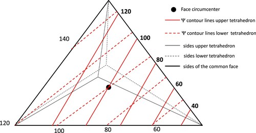
In PS and CS1, the pressure gradient B is kept constant. In CS2, its correction is computed as the solution of a conservative problem, where the velocity is opposite to the pressure gradient. We will show in the following that, at the end of each step PS, CS1 and CS2, the computed velocity is piece-wise constant in each element, but the fluxes $Q_j^e$ in Equation (9) are opposite at the common face of two neighboring elements only at the end of CS2. Assuming a piece-wise linear pressure as initial condition, because the CS2 velocity correction is conservative with respect to the pressure correction, the pressure gradient remains piece-wise constant in all the steps. It can also be shown that the pressure correction computed in CS2 step by the MHFE is continuous along the element faces only in their circumcenters. Because pressure changes only in CS2 step, the same condition holds also for the pressure at the end of each time step. See in Figure 1 the pressure contour lines inside the face common to two neighboring tetrahedrons.

Figure 1. RT0 kinematic pressure contour lines in the face common to two tetrahedrons.

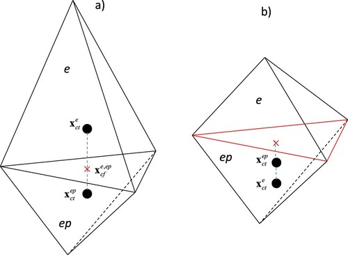
The presentation of the solution of each step in Equations (8) is restricted first to the hypothesis of a mesh with an Extended Delaunay Property (EDP), as defined in Aricò et al. (2011), and then generalized in section 4 to the case of totally irregular meshes. In an EDP mesh, the circumsphere of any tetrahedron does not include any other node inside it (Forsyth, 1991; Joe, 1986; Letniowski, 1992) and, with reference to Figure 2, the following conditions hold for two neighboring tetrahedrons e and ep, (10a) $\begin{array}{rl}& ({\mathbf{\text{v}}}_2-{\mathbf{\text{v}}}_1)\cdot {\mathbf{\text{v}}}_1<0\text{ if}|{\mathbf{\text{v}}}_1|>|{\mathbf{\text{v}}}_2|\end{array}$(10a) (10b) $\begin{array}{rl}& ({\mathbf{\text{v}}}_1-{\mathbf{\text{v}}}_2)\cdot {\mathbf{\text{v}}}_2<0\text{ if}|{\mathbf{\text{v}}}_2|>|{\mathbf{\text{v}}}_1|\end{array}$(10b) where vectors v₁ and v₂ are defined as (10c) ${\mathbf{\text{v}}}_1=({\mathbf{\text{x}}}_{ct}^e-{\mathbf{\text{x}}}_{cf}^{e,ep}),{\mathbf{\text{v}}}_2=({\mathbf{\text{x}}}_{ct}^{ep}-{\mathbf{\text{x}}}_{cf}^{e,ep})$(10c) ${\mathbf{\text{x}}}_{ct}^{e(ep)}$ is the coordinate vector of the circumcenter of tetrahedron e (ep), ${\mathbf{\text{x}}}_{cf}^{e,ep}$ is the coordinate vector of the circumcenter of the face shared by tetrahedrons e and ep. Moreover, the following condition holds for the boundary elements e and the corresponding boundary face (11) $\mathbf{\text{v}}\cdot \mathbf{\text{n}}<0$(11) where n is the unit vector normal to the boundary face and oriented in the outward direction, v is defined as (12) $\mathbf{\text{v}}=({\mathbf{\text{x}}}_{ct}^e-{\mathbf{\text{x}}}_{cf}^e)$(12) and ${\mathbf{\text{x}}}_{cf}^e$ is the coordinate vector of the circumcenter of the boundary face. In Figure 2(a,b), tetrahedrons e and ep satisfy and do not satisfy the EDP, respectively.

Figure 2. (a) The two tetrahedrons e and ep satisfy the EDP. (b) The two tetrahedrons do not satisfy the EDP.

We will prove in the next sections that in an EDP mesh the system matrix, associated with the solution of the steps (8b) and (8c), is an M-matrix (Letniowski, 1992), and this avoids nonphysical local extrema in the computed solution (Forsyth, 1991; Letniowski, 1992). The same matrix property will be saved in the more general case of non-Delaunay meshes by changing the control volumes of the momentum equations, as will be shown in section 4.

3. MAST-RT0 solution in the case of Delaunay meshes

3.1. Prediction step

The step (8a) is solved by assuming, in each tetrahedral element, constant viscous and pressure gradient forces and by integrating convective inertial terms according to the MArching in Space and Time (MAST) procedure. MAST computes the solution of convective problems, with only one characteristic line passing through each (x, t) point of the domain, in the framework of a fractional time step procedure.

In MAST the three discretized momentum equations are solved in each element, uncoupled from the other ones. To this end, at the beginning of each k^th time step, all the elements are marked with an index $R_e^k$∈R^k, called ‘rank’. The rank of an element e is an integer which is a unit greater than the ranks of all the neighboring ep elements with a common face crossed by a flux entering element e from element ep. All the elements are initialized at the beginning of each new time iteration with rank zero, and vector R^k is computed starting from the boundary elements with all interior fluxes oriented outward, which are set with rank 1. The rank is then computed for the elements that are neighbors to elements with rank greater than zero and have no interior faces crossed by fluxes oriented inward. The procedure is continued until all the elements of the computational domain have rank greater than zero. After computation of R^k, all the elements are sorted according to increasing rank values and solved one after the other.

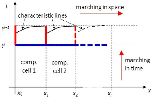
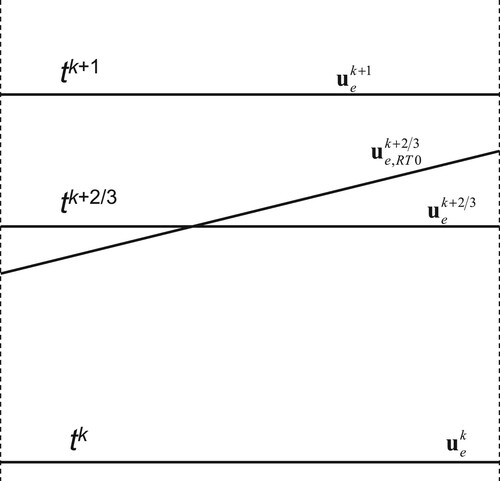
During the solution of element e, the integral of the velocity momentum is computed and the mean momentum fluxes are added as external forces to the neighboring elements ep with entering flux and higher rank. The MAST solution of the prediction problem along time step k can be viewed as a reduction of the computational domain carried out after the solution of each boundary element, through extraction of the latter. This reduction makes it possible to solve originally internal elements according to the information carried on by characteristic lines rooted at the boundary of internal elements that behave like domain boundaries. In the example of Figure 3, cell 1 is solved using the information at x₀ carried on by the first characteristic line. After interpolation in time of the solution at the cell boundary in x₁, the second cell is solved using information carried on by the second characteristic line rooted between t^k and t^k+1 at x₁. In this way, the sought after solution is not subject to the Courant restriction on the maximum size of the time step.

Figure 3. Sketch of MAST algorithm in the 1D case.

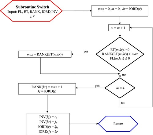
In Aricò et al. (2013b) it has been shown that the basic requirement for the application of the MAST algorithm is the existence of a continuous ‘anisotropic scalar potential’ P of the flow field, such that the velocity can be computed as (13) $\mathbf{\text{u}}=-{\mathbf{\text{K}}}_0\mathrm{\nabla }P$(13) where K₀ is a (3 × 3) positive-definite tensor. In the same paper it is shown that for any incompressible and viscous fluid this potential always exists and streamlines are always open but, due to numerical discretization, it is possible in the computed velocity field to get one or more loops where a single element without a flux entering from other elements of the same loop does not exist. In this condition the rank vector cannot be computed and, to apply MAST, we need to select a ‘cut’ face between two elements of the same loop with a small flux, which has to be assumed constant during the time step and equal to its initial value. See in Appendix 1 a very fast procedure, named Order, aimed to compute the R^k vector, where the flux entering from the ‘cut’ face of a loop is treated as a known boundary flux. After application of the Order algorithm, an open source subroutine ‘QUICKSORT’ in the package KB07¹ can be used to order the elements according to their rank values.

After integration in space, the prediction step of Equation (7a) can be written, for any element e, as (14) $\begin{array}{rl}& {\int }_{W_e}\frac{\mathrm{\partial }\mathbf{\text{u}}}{\mathrm{\partial }t}dw+{\int }_{W_e}\mathbf{\text{u}}\cdot \mathrm{\nabla }\mathbf{\text{u}}dw+{\int }_{W_e}\mathrm{\nabla }{\mathrm{\Psi }}^{k}dw\\ & -\nu {\int }_{W_e}{\mathrm{\nabla }}_2{\mathbf{\text{u}}}^{k-1/3}dw=0e=1,\dots ,N_T\end{array}$(14) with the symbols specified as above. The first and second terms on the l.h.s. of Equation (14) represent the local and convective inertial terms, respectively, the third term is the force over the element due to the gradient of the kinematic pressure and the last term accounts for the effect of the viscous forces.

From now on we will call j (in the local element reference, j = 1, … , 4) the face that tetrahedron e shares with its neighboring ep, and jp (in a local reference too) the face that ep shares with e. The symbols ${\sigma }_j^e$ and n_j represent the area and the unit outward orthogonal vector of the jth face of tetrahedron e, respectively.

Due to the cell sorting operation at the beginning of each time iteration, the solution of the momentum Equation (14) for element e with rank $R_e^k$, depends (a) on the incoming momentum fluxes from neighboring ep elements with $R_{ep}^k$ < $R_e^k$, (b) on the kinematic pressure gradients and viscous terms, which are known from the solution of the previous time step, and (c) on the initial solution inside the element at the beginning of the new time step. For these reasons, the PDEs system in Equation (14) can be regarded as a small (3 × 3) Ordinary Differential Equations (ODEs) system to be solved for the velocity components in element e.

Starting from a piecewise constant in space (P₀) and divergence-free velocity distribution inside each tetrahedron e, ${\mathbf{\text{u}}}_e^k\in {\mathbf{\text{X}}}_e$ and ${\mathbf{\text{u}}}_e^k\in P_{0,e}$, we assume that at the generic time τ inside the time step (0 $\le$ τ $\le$ Δt) the velocity value is (15) ${\mathbf{\text{u}}}_e(\tau )={\mathbf{\text{u}}}_e^k+\mathrm{\Delta }{\mathbf{\text{u}}}_e^f(\tau )$(15) where $\mathrm{\Delta }{\mathbf{\text{u}}}_e^f(\tau )\in P_{0,e}$ and $\mathrm{\Delta }{\mathbf{\text{u}}}_e^f(0)$=0. Applying the Green lemma to the second integral on the l.h.s. of Equation (14), the equilibrium ODEs system for tetrahedron e can be written as (16) $\begin{array}{rl}& \frac{d(\mathrm{\Delta }{\mathbf{\text{u}}}_e^f)}{d\tau }{W}_e+\sum _{j=1,4}{\phi }_j^e{\mathbf{\text{M}}}_j^{e,out}(\tau )+\sum _{j=1,4}(1-{\phi }_j^e){\overline{\mathbf{\text{M}}}}_j^{e,in}\\ & +{\mathbf{\text{S}}}_{\mathrm{\Psi },e}^k+{\mathbf{\text{VF}}}_e^{k-1/3}=0e=1,\dots ,N_T\end{array}$(16) where ${\mathbf{\text{M}}}_j^{e,out}(\tau )$ is the leaving momentum flux from tetrahedron e to the neighboring tetrahedron ep, ${\overline{\mathbf{\text{M}}}}_j^{e,in}$ is the mean incoming momentum flux entering tetrahedron e crossing the jth face, computed along with the solution of the previous elements, ${\phi }_j^e$ = 1 for faces shared by elements with higher rank or boundary faces with positive flux, otherwise ${\phi }_j^e$ = 0. ${\mathbf{\text{S}}}_{\mathrm{\Psi },e}^k$ and ${\mathbf{\text{VF}}}_e^{k-1/3}$ are the sum of the kinematic pressure and the viscous forces over the four faces of tetrahedron e, respectively, computed in the previous time step as specified in sections 3.2 and 3.3. ODEs systems (16) are sequentially solved, one for each element, starting from the tetrahedrons with the smallest $R_e^k$ value, and proceeding to the tetrahedrons with higher $R_e^k$ values. We call this step MAST forward step (MAST-fs). To solve system (16) from time 0 to time Δt, we use an explicit Runge–Kutta (RK) code (Brankin et al., 1993). This code adopts an internal time sub-grid, selected within the interval [0 – Δt], on which the approximate ODEs solution is computed. The position of the nodes of the grid is automatically selected by the RK code according to a local error estimation (Brankin et al., 1993).

Due to the change of the velocity vector during the ODEs system solution we could obtain, in intermediate times between 0 and Δt, momentum fluxes moving from the element e into other ep elements with a lower rank ($R_{ep}^k$ < $R_e^k$). To avoid this, we approximate the leaving momentum flux in the MAST-fs forward step as (17) ${\mathbf{\text{M}}}_j^{e,out}(\tau )={\sigma }_j^e{\mathbf{\text{u}}}_e(\tau )max[0,{\mathbf{\text{u}}}_e(\tau )\cdot {\mathbf{\text{n}}}_j]$(17) with the symbols specified above. To restore the force integral neglected in the integration of Equation (14) due to the limit of the momentum flux assigned in Equation (17), after the end of the forward step we again perform the solution of the 3-ODEs system in sequential way, assuming as initial u_e value the one computed at the end of the MAST-fs forward step. In MAST backward solution (MAST-bs) we start from the tetrahedrons with the highest $R_e^k$ value and proceed to the tetrahedrons with smaller $R_e^k$ values, saving only the inertial terms of Equation (14), that is: (18a) $\begin{array}{rl}& \frac{d(\mathrm{\Delta }{\mathbf{\text{u}}}_e^b)}{d\tau }{W}_e+\sum _{j=1,4}(1-{\phi }_j^e){\mathbf{\text{M}}}_j^{e,out}(\tau )\\ & +\sum _{j=1,4}{\phi }_j^e{\overline{\mathbf{\text{M}}}}_j^{e,in}=0\end{array}$(18a) (18b) $\begin{array}{rl}& {\mathbf{\text{u}}}_e(\tau )={\mathbf{\text{u}}}_e^k+\mathrm{\Delta }{\mathbf{\text{u}}}_e^f(\mathrm{\Delta }t)+\mathrm{\Delta }{\mathbf{\text{u}}}_e^b(\tau )\end{array}$(18b) where $\mathrm{\Delta }{\mathbf{\text{u}}}_e^b(\tau )\in P_{0,e}$, $\mathrm{\Delta }{\mathbf{\text{u}}}_e^b(0)=0$, and the momentum fluxes ${\mathbf{\text{M}}}_j^{e,out}(\tau )$ are computed as for the forward step.

During the solution of the ODEs system (16) or (18), we compute the solution at n_G selected number of Gauss integration points chosen in the interval [0 – Δt].

At the end of the solution of each ODEs system (16) or (18), in the MAST-fs and MAST-bs problems we compute the momentum fluxes coming into element e from the neighboring ep tetrahedrons as (19) $\begin{array}{rl}& {\overline{\mathbf{\text{M}}}}_j^{e,in}=-{\overline{\mathbf{\text{M}}}}_{jp}^{ep,out}\end{array}$(19) (20a) $\begin{array}{rl}& {\overline{\mathbf{\text{M}}}}_{jp}^{ep,out}=\sum _{l=1,n_G}\frac{{\phi }_{jp}^{ep}{\sigma }_{jp}^{ep}max[0,{\mathbf{\text{u}}}_{ep}({\tau }_l)\cdot {\mathbf{\text{n}}}_j]}{\sum _{m=1,4}\{{\phi }_m^{ep}{\sigma }_m^{ep}max[0,{\mathbf{\text{u}}}_{ep}({\tau }_l)\cdot {\mathbf{\text{n}}}_m]\}}\\ & \times {\mathbf{\text{M}}}_{jp}^{ep,out}({\tau }_l)w_l\text{ in MAST - fs}\end{array}$(20a) (20b) $\begin{array}{rl}& {\overline{\mathbf{\text{M}}}}_{jp}^{ep,out}\\ & =\sum _{l=1,n_G}\frac{(1-{\phi }_{jp}^{ep}){\sigma }_{jp}^{ep}max[0,{\mathbf{\text{u}}}_{ep}({\tau }_l)\cdot {\mathbf{\text{n}}}_{jp}]}{\sum _{m=1,4}\{(1-{\phi }_m^{ep}){\sigma }_m^{ep}max[0,{\mathbf{\text{u}}}_{ep}({\tau }_l)\cdot {\mathbf{\text{n}}}_m]\}}\\ & \times {\mathbf{\text{M}}}_{jp}^{ep,out}({\tau }_l)w_l\text{ in MAST - bs}\end{array}$(20b) where τ _l and w_l are the time and the weight associated with the l^th Gauss point, with 1 $\le$ l $\le$n_G.

The final velocity u^k+1/3 is computed by Equation (18b) for τ =Δt. u^k+1/3 is piecewise constant and divergence-free inside each tetrahedron (${\mathbf{\text{u}}}_e^{k+1/3}\in P_{0,e}$), but the fluxes crossing the same face of two neighboring elements will not be opposite for the two elements in the computed solution and this disrupts mass conservation at time level t^k+1/3.

In the MAST-fs problem, we compute the boundary momentum fluxes of tetrahedron e, different from zero, as (21a) $\begin{array}{rl}{\mathbf{\text{M}}}_j^{e,in}(\tau )& ={\sigma }_j^e{\mathbf{\text{g}}}_{j,e}(\tau )({\mathbf{\text{g}}}_{j,e}(\tau )\cdot {\mathbf{\text{n}}}_j)\\ & \text{if }({\mathbf{\text{g}}}_{j,e}(\tau )\cdot {\mathbf{\text{n}}}_j\le 0\text{ and }j\in {\mathrm{\Gamma }}_u)\end{array}$(21a) (21b) $\begin{array}{rl}{\mathbf{\text{M}}}_j^{e,in}(\tau )& ={\sigma }_j^e{\mathbf{\text{u}}}_e(\tau )min(0,{\mathbf{\text{u}}}_e(\tau )\cdot {\mathbf{\text{n}}}_j)\\ & \text{if }({\mathbf{\text{u}}}_e^k\cdot {\mathbf{\text{n}}}_j\le 0\text{ and }j\in {\mathrm{\Gamma }}_{\sigma })\end{array}$(21b) (21c) $\begin{array}{rl}{\mathbf{\text{M}}}_j^{e,out}(\tau )& ={\sigma }_j^e{\mathbf{\text{u}}}_e(\tau )max(0,{\mathbf{\text{u}}}_e(\tau )\cdot {\mathbf{\text{n}}}_j)\text{ if }({\mathbf{\text{u}}}_e^k\cdot {\mathbf{\text{n}}}_j\ge 0\end{array}$(21c) where g_j,e is the velocity vector assigned on the face j ∈ Γ_u of element e.

In the MAST-bs problem, we compute the same fluxes as (22a) $\begin{array}{rl}{\mathbf{\text{M}}}_j^{e,in}(\tau )& ={\sigma }_j^e{\mathbf{\text{u}}}_e(\tau )min(0,{\mathbf{\text{u}}}_e(\tau )\cdot {\mathbf{\text{n}}}_j)\\ & \text{if }({\mathbf{\text{u}}}_e^k\cdot {\mathbf{\text{n}}}_j>0\text{ and }j\in {\mathrm{\Gamma }}_{\sigma })\end{array}$(22a) (22b) $\begin{array}{rl}{\mathbf{\text{M}}}_j^{e,out}(\tau )& ={\sigma }_j^e{\mathbf{\text{u}}}_e(\tau )max(0,{\mathbf{\text{u}}}_e(\tau )\cdot {\mathbf{\text{n}}}_j)\text{ if }{\mathbf{\text{u}}}_e^k\cdot {\mathbf{\text{n}}}_j<0\end{array}$(22b)

3.1.1. Parallel solution of the MAST prediction step

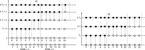
The solution of the MAST PS in 1D problems is inherently serial and cannot be achieved with parallel computing. On the opposite, in 2D and 3D problems it could be possible to carry out simultaneously the solution of all the elements with the same rank using several CPU physical processors, just saving the average entering momentum fluxes computed for each element in both the forward and backward steps. See in Figure 4(a) the scheme of the MAST-fs solution, for a computer with five processors, of a single time step of a model with 13 elements, ordered in two groups of rank 1 (7 elements) and rank 2 (6 elements). The white circles represent the initial value of the variables and the black circles the final one. T_T is the computational time required to each processor for the solution of one element. Observe that, due to the need of solving all the elements with rank 1, before proceeding to the other ones, some processors have to solve 4 elements before moving to the next time step, where in any traditional marching in time method (MTM) only a maximum of 3 elements would be required, as shown in Figure 4(b). An additional time ϵ is also required, for each time step, for the rank computation and the element ordering in the MAST-fs (see Figure 4(a)). These last operations, as better specified in the tests run in section 5 with millions of elements, require a computational time two or three order of magnitude smaller than T_T.

Figure 4. Solution of a single time step. (a) Scheme of the parallel solution of the MAST-fs (or MAST-bs). (b) Scheme of the parallel solution of traditional MArching in Time method (MTM).

For meshes with at least a few hundred thousand elements, the maximum number N_r,k of elements within a single rank $R_e^k$ at time step k is usually much larger than the available physical processors in standard computers. For test 3 (in section 5.3.3), we estimate N_r,k and predict the corresponding computational time of parallelization of the MAST algorithm for different number of processors.

3.2. The CS1 correction step

By integrating Equation (8b) in space, we obtain the following system, to be solved for the three unknown velocity components ${\mathbf{\text{u}}}_e^{k+2/3}\in P_{0,e}$, from time level t^k+1/3 to time level t ^k+2/3, (23) $\begin{array}{rl}& \frac{{\mathbf{\text{u}}}_e^{k+2/3}-{\mathbf{\text{u}}}_e^{k+1/3}}{\Delta t}{W}_e-{\int }_{W_e}\nu {\Delta }_2{\mathbf{\text{u}}}_e^{k+2/3}dw\\ & =-{\int }_{W_e}\nu {\Delta }_2{\mathbf{\text{u}}}_e^{k-1/3}dwe=1,\dots ,N_T\end{array}$(23)

Application of the Green lemma to the volume integral on the l.h.s. of Equation (23) leads to (24) $\begin{array}{rl}-\nu {\int }_{W_e}{\Delta }_2{\mathbf{\text{u}}}_e^{k+2/3}dw& =-\nu \sum _{j=1,4}{\sigma }_j^e\frac{\mathrm{\partial }{\mathbf{\text{u}}}_e^{k+2/3}}{\mathrm{\partial }n}\\ & =\nu \sum _{j=1,4}{\sigma }_j^e\frac{{\mathbf{\text{u}}}_e^{k+2/3}-{\mathbf{\text{u}}}_{ep}^{k+2/3}}{d_{e,ep}}\end{array}$(24) where $\frac{\mathrm{\partial }\mathbf{\text{u}}}{\mathrm{\partial }n}$ is the derivative of the velocity vector along the direction orthogonal to face ${\sigma }_j^e$, d_e,ep is the distance of the circumcenters of the two neighboring tetrahedrons e and ep, computed as specified in Equation (25), and the other symbols have already been defined. We compute the distance as (25) $\begin{array}{rl}& d_{e,ep}=(|{\mathbf{\text{v}}}_1-{\mathbf{\text{v}}}_2|)sign\\ & \text{where }sign\\ & =1\text{ if }\{\begin{array}{l}(({\mathbf{\text{v}}}_2-{\mathbf{\text{v}}}_1)\cdot {\mathbf{\text{v}}}_1\\ <0\text{.and}\text{. }|{\mathbf{\text{v}}}_1|>|{\mathbf{\text{v}}}_2|)\\ \text{.or}\text{.}\\ (({\mathbf{\text{v}}}_1-{\mathbf{\text{v}}}_2)\cdot {\mathbf{\text{v}}}_2\\ <0\text{.and}\text{. }|{\mathbf{\text{v}}}_2|>|{\mathbf{\text{v}}}_1|)\end{array}\begin{array}{l}sign=-1\\ \text{ otherwise }\end{array}\end{array}$(25) where vectors v₁ and v₂ have been defined in Equation (10c). For each tetrahedron e we set (26) $\mathrm{\Delta }{\stackrel{⌢}{\mathbf{u}}}_{\mathbf{e}}={\mathbf{\text{u}}}_e^{k+2/3}-{\mathbf{\text{u}}}_e^{k+1/3}\text{ with }\mathrm{\Delta }{\stackrel{⌢}{\mathbf{u}}}_{\mathbf{e}}\in P_{0,e}$(26) such that the r.h.s. of Equation (24) becomes, (27) $\begin{array}{rl}& \nu {\sigma }_j^e\frac{{\mathbf{\text{u}}}_e^{k+2/3}-{\mathbf{\text{u}}}_{ep}^{k+2/3}}{d_{e,ep}}\\ & =\nu {\sigma }_j^e\left(\frac{{\mathbf{\text{u}}}_e^{k+1/3}-{\mathbf{\text{u}}}_{ep}^{k+1/3}}{d_{e,ep}}+\frac{\mathrm{\Delta }{\stackrel{⌢}{\mathbf{u}}}_e-\mathrm{\Delta }{\stackrel{⌢}{\mathbf{u}}}_{ep}}{d_{e,ep}}\right)\end{array}$(27)

On the r.h.s. of Equation (23) we assume (28) $\begin{array}{rl}-\nu {\int }_{W_e}{\Delta }_2{\mathbf{\text{u}}}_e^{k-1/3}dw& \simeq -\nu {\int }_{W_e}{\Delta }_2{\mathbf{\text{u}}}_e^{k}dw\\ & =\nu \sum _{j=1,4}{\sigma }_j^e\frac{{\mathbf{\text{u}}}_e^k-{\mathbf{\text{u}}}_{ep}^k}{d_{e,ep}}\end{array}$(28)

We set (29) $\mathrm{\Delta }{\widetilde{\mathbf{\text{u}}}}_e={\mathbf{\text{u}}}_e^{k+1/3}-{\mathbf{\text{u}}}_e^k\text{with}\mathrm{\Delta }{\widetilde{\mathbf{\text{u}}}}_e\in P_{0,e}$(29) and merging Equation (29) with Equation (27) we get (30) $\begin{array}{rl}& \nu {\sigma }_j^e\frac{{\mathbf{\text{u}}}_e^{k+1/3}-{\mathbf{\text{u}}}_{ep}^{k+1/3}}{d_{e,ep}}\\ & =\nu {\sigma }_j^e\left(\frac{{\mathbf{\text{u}}}_e^k-{\mathbf{\text{u}}}_{ep}^k}{d_{e,ep}}+\frac{\mathrm{\Delta }{\widetilde{\mathbf{\text{u}}}}_e-\mathrm{\Delta }{\widetilde{\mathbf{\text{u}}}}_{ep}}{d_{e,ep}}\right)\end{array}$(30)

According to Equations (26)-(30), system (30) can be rewritten as (31) $\begin{array}{rl}& \frac{\mathrm{\Delta }{\stackrel{⌢}{\mathbf{u}}}_e}{\Delta t}{W}_e+\nu \sum _{j=1,4}{\sigma }_j^e\frac{\mathrm{\Delta }{\stackrel{⌢}{\mathbf{u}}}_e-\mathrm{\Delta }{\stackrel{⌢}{\mathbf{u}}}_{ep}}{d_{e,ep}}\\ & =\nu \sum _{j=1,4}{\sigma }_j^e\frac{\mathrm{\Delta }{\widetilde{\mathbf{\text{u}}}}_e-\mathrm{\Delta }{\widetilde{\mathbf{\text{u}}}}_{ep}}{d_{e,ep}}\end{array}$(31) and solved for the components of the velocity correction $\mathrm{\Delta }{\stackrel{⌢}{\mathbf{u}}}_{\mathbf{e}}$.

The matrix of system (31) is sparse, symmetric and positive definite, with diagonal and off-diagonal coefficients $M_{e,e}^{C{S}_1}$ and $M_{e,ep}^{C{S}_1}$ equal to (32) $M_{e,e}^{C{S}_1}=\frac{W_e}{\Delta t}+\nu \sum _{j=1,4}{\sigma }_j^e\frac{1}{d_{e,ep}},M_{e,ep}^{C{S}_1}=-\nu {\sigma }_j^e\frac{1}{d_{e,ep}}$(32) and the e-th element of the source term vector is the r.h.s. of Equation (31).

For the boundary face j $\in$ Γ_u of tetrahedron e, the velocity at the circumcenter of the neighboring tetrahedron is replaced in the system of Equation (31) by the boundary velocity at the circumcenter of the boundary face and the distance d_e,ep with the distance $d_j^e$ between the tetrahedron and the face circumcenter, defined as (33) $d_j^e=-\mathbf{\text{v}}\cdot \mathbf{\text{n}}$(33) where v and n have been already defined in Equations (11) and (12). If the boundary face belongs to Γ_u and condition ${\mathbf{\text{g}}}_{j,e}(t^{k+1/3})\cdot {\mathbf{\text{n}}}_j\le 0$ holds, the velocity correction $\mathrm{\Delta }{\stackrel{⌢}{\mathbf{u}}}_{\mathbf{j}}$ at the boundary face, from t^k+1/3 to t^k+2/3, is (34a) $\begin{array}{rl}\mathrm{\Delta }{\stackrel{⌢}{\mathbf{u}}}_{\mathbf{j}}& ={\mathbf{\text{g}}}_{j,e}(t^{k+2/3})-{\mathbf{\text{g}}}_{j,e}(t^{k+1/3})\\ & ={\mathbf{\text{g}}}_{j,e}(t^k+\mathrm{\Delta }t)-{\mathbf{\text{g}}}_{j,e}(t^k+\mathrm{\Delta }t)\end{array}$(34a) equal to zero along with the corresponding off-diagonal matrix coefficient in Equation (32), and the contribution to the source term becomes (34b) $\mathrm{\Delta }{\widetilde{\mathbf{\text{u}}}}_j={\mathbf{\text{g}}}_{j,e}(t^{k+1/3})-{\mathbf{\text{g}}}_{j,e}(t^k)={\mathbf{\text{g}}}_{j,e}(t^k+\mathrm{\Delta }t)-{\mathbf{\text{g}}}_{j,e}(t^k)$(34b)

If the boundary face belongs to Γ_u and condition ${\mathbf{\text{g}}}_{j,e}(t^{k+1/3})\cdot {\mathbf{\text{n}}}_j>0$ holds, the boundary velocity at time t^k+1/3 is assumed to be the tetrahedral element velocity ${\mathbf{\text{u}}}_e^{k+1/3}$, that implies $\mathrm{\Delta }{\stackrel{⌢}{\mathbf{u}}}_{\mathbf{j}}={\mathbf{\text{g}}}_{j,e}(t^k+\mathrm{\Delta }t)-{\mathbf{\text{u}}}_e^{k+1/3}$ and (35) $\mathrm{\Delta }{\widetilde{\mathbf{\text{u}}}}_j={\mathbf{\text{u}}}_e^{k+1/3}-{\mathbf{\text{u}}}_e^k$(35)

If the boundary face belongs to Γ_σ or to Γ_m, for simplicity’s sake we neglect the viscous tangent stress components, along with the terms in Equation (31) proportional to the viscosity.

If the EDP is satisfied (see section 2), due to Equations (11)-(12), the diagonal and off-diagonal coefficients in Equation (32) are positive and non-positive, respectively, such that the M-matrix property of the matrix is always guaranteed (Forsyth, 1991; Letniowski, 1992).

We adopt a preconditioned conjugate gradient method to solve system (31), using incomplete Cholesky factorization² and a compressed row storage (CRS) format, which makes it possible to save a lot of computational memory allocation (we store the main diagonal and the upper off-diagonal matrix coefficients). Since the matrix coefficients only depend on the geometrical variables, as well as the value of the kinematic viscosity, the matrix is only factorized once, before the time iterations loop starts, and this makes it possible to save a lot of computational effort.

After system (31) is solved, the velocity in each tetrahedron is updated according to Equation (26). At time level t^k+2/3 for each tetrahedron e we compute the sum ${\mathbf{\text{FV}}}_e^{k+2/3}$ of the viscous forces over its four faces as (36) ${\mathbf{\text{FV}}}_e^{k+2/3}=\sum _{j=1,4}\nu {\sigma }_j^e\frac{{\mathbf{\text{u}}}_e^{k+2/3}-{\mathbf{\text{u}}}_{ep}^{k+2/3}}{d_{e,ep}}$(36) and we neglect the change in it occurring along the next CS2 correction step.

At the end of the CS1 problem, the continuity of the fluxes crossing the same face of two neighboring elements e and ep is not yet restored, and, similarly to ${\mathbf{\text{u}}}_e^{k+1/3}$ at the end of the PS problem (section 3.1), ${\mathbf{\text{u}}}_e^{k+2/3}\in P_{0,e}$, but mass conservation is not satisfied.

The spatial discretization of the derivative $\frac{\mathrm{\partial }\mathbf{\text{u}}}{\mathrm{\partial }n}$ proposed in Equation (24) is similar to the one presented by Younes et al. (2004, 2006) for the 2D Mixed Hybrid Finite Element method lumped in the circumcenter of triangles. Unlike the formulation of the present work, Younes et al. (2004) proved that their corresponding 3D discretization exists only for regular tetrahedrons, and cannot be extended to a general 3D tetrahedral discretization.

3.3. The CS2 correction step

Substituting Equations (5b) in Equations (8c), we get (37) $\frac{{\mathbf{\text{u}}}^{k+1}-{\mathbf{\text{u}}}^{k+2/3}}{\Delta t}+\mathrm{\nabla }({\mathrm{\Psi }}^{k+1}-{\mathrm{\Psi }}^k)=0$(37) which has to be solved to restore the flux continuity disrupted in the prediction and in the first correction steps. To this end we set (38) ${\mathbf{\text{u}}}^{k+1}-{\mathbf{\text{u}}}_{RT0}^{k+2/3}=\mathrm{\nabla }\eta \mathrm{\Delta }t$(38) where η is an unknown function with the same dimensions as ψ, and ${\mathbf{\text{u}}}_{RT0}^{k+2/3}\in {\mathbf{\text{X}}}_e$ is the RT0 velocity at time level t^k+2/3 computed by Equation (9) in each tetrahedron e as function of the weight mean flux ${\overline{Fl}}_{e,j}^{k+2/3}$ through face j of e, given by (39) ${\overline{Fl}}_{j,e}^{k+2/3}=\frac{F{l}_{j,e}^{k+2/3}{W}_{ep}-F{l}_{jp,ep}^{k+2/3}{W}_e}{W_e+W_{ep}}j,jp=1,\dots ,4$(39) where $F{l}_{j,e}^{k+2/3}$ is the flux due to velocity ${\mathbf{\text{u}}}_e^{k+2/3}$ crossing face j of e, and $F{l}_{jp,ep}^{k+2/3}$ is the flux due to velocity ${\mathbf{\text{u}}}_{ep}^{k+2/3}$ crossing the same face jp of ep. From Equation (39), flux ${\overline{Fl}}_{j,e}^{k+2/3}$ is opposite for the two neighboring tetrahedrons e and ep and the weight of each flux is inversely proportional to the volume of the corresponding element. Because the common face can be thought of as the basis of the two tetrahedrons, this is equivalent to assuming an inverse proportionality of the flux with respect to the corresponding height of the tetrahedron. According to Equation (9), we get (40) ${\mathbf{\text{u}}}_{e,RT0}^{k+2/3}=\sum _{j=1,4}{\mathit{\omega }}_j^e{\overline{Fl}}_{j,e}^{k+2/3}$(40) with the symbols already specified. Since the sum of the four fluxes $F{l}_{j,e}^{k+2/3}$ j = 1, … , 4 is not zero, mass conservation is not satisfied by the ${\mathbf{\text{u}}}_{RT0}^{k+2/3}$ velocity field in tetrahedron e, $\mathrm{\nabla }\cdot {\mathbf{\text{u}}}_{RT0}^{k+2/3}\ne 0$ and ${\mathbf{\text{u}}}_{RT0}^{k+2/3}\in P_{1,e}$ (piecewise linear inside the tetrahedrons), as explained in section 2.2. By subtracting u^k from both members in Equation (38), we get (41) $\mathrm{\nabla }\eta \mathrm{\Delta }t+{\mathbf{\text{u}}}_{RT0}^{k+2/3}-{\mathbf{\text{u}}}^k={\mathbf{\text{u}}}^{k+1}-{\mathbf{\text{u}}}^k$(41) Taking the divergence of Equation (41), we get (42) $\mathrm{\Delta }t{\mathrm{\nabla }}^2\eta +\mathrm{\nabla }\cdot ({\mathbf{\text{u}}}_{RT0}^{k+2/3}-{\mathbf{\text{u}}}^k)=\mathrm{\nabla }\cdot ({\mathbf{\text{u}}}^{k+1}-{\mathbf{\text{u}}}^k)$(42)

Integration of Equation (42) and application of the Green lemma leads to (43) $\mathrm{\Delta }t\sum _{j=4}{\sigma }_j^e\frac{{\eta }_e-{\eta }_{ep}}{d_{e,ep}}+\sum _{j=4}({\overline{Fl}}_{j,e}^{k+2/3}-F{l}_{j,e}^k)=F{l}_e$(43) where the first term is the flux of the vector ${\mathbf{\text{u}}}^{k+1}-{\mathbf{\text{u}}}_{RT0}^{k+2/3}$, ${\overline{Fl}}_{j,e}^{k+2/3}$ is defined in Equation (39), $F{l}_{j,e}^k$ is the flux crossing face j of element e due to velocity ${\mathbf{\text{u}}}^k\in {\mathbf{\text{X}}}_e$ and Fl_e is the total flux of the vector (u^k+1-u^k) crossing the surface of element e. For the gradient of η we adopt the spatial discretization already applied in section 3.2 for the velocity gradient (see Equation (24)).

To compute η, we impose the condition that both u^k+1 and u^k are divergence-free, with ${\mathbf{\text{u}}}^{k+1}\in {\mathbf{\text{X}}}_e$ and ${\mathbf{\text{u}}}^{k+1}\in P_{0,e}$, which implies that in Equation (43) the flux Fl_e of the velocity (u^k+1 – u^k) crossing the total surface of the tetrahedron is zero (see in Figure 5 a 1D sketch of velocity vectors inside tetrahedron e). The resulting system is (44) $\mathrm{\Delta }t\sum _{j=4}{\sigma }_j^e\frac{{\eta }_e-{\eta }_{ep}}{d_{e,ep}}+\sum _{j=4}({\overline{Fl}}_{j,e}^{k+2/3}-F{l}_{j,e}^k)=0$(44)

Figure 5. 1D sketch of velocity vectors inside tetrahedron e.

Equations (44) form a well-conditioned linear system to be solved for the η unknowns. The matrix of the system is sparse, symmetric and positive-definite. Diagonal and off-diagonal coefficients $M_{e,e}^{C{S}_2}$ and $M_{e,ep}^{C{S}_2}$ are, respectively, (45a) $M_{e,e}^{C{S}_2}=\sum _{j=1,4}{\sigma }_j^e\frac{\mathrm{\Delta }t}{d_{e,ep}},M_{e,ep}^{C{S}_2}=-{\sigma }_j^{ep}\frac{\mathrm{\Delta }t}{d_{e,ep}}$(45a) and the same M-property of the coefficients of the matrix of the system of CS1 holds (see section 3.2). The e-th coefficient of the source term vector is (45b) $S{t}_e^{C{S}_2}=-\sum _{j=4}({\overline{Fl}}_{j,e}^{k+2/3}-F{l}_{j,e}^k)$(45b)

The solution of system (44)-(45) is performed in the same way as for system (31)-(32). In the present case too, matrix coefficients only depend on the geometrical variables and time step size, so that the system matrix is factorized only once before the time iteration loop starts, saving a lot of computational time.

We call (46) $F{l}_{j,e}^{\eta }=\mathrm{\Delta }t{\sigma }_j^e\frac{{\eta }_e-{\eta }_{ep}}{d_{e,ep}}$(46) the flux crossing face j of e due to the gradient of η. This flux is continuous for the two neighboring elements e and ep, with $F{l}_{j,e}^{\eta }=-F{l}_{jp,ep}^{\eta }$. For the tetrahedron e we compute the final velocity at time level t^k+1 from the fluxes on the l.h.s. of Equations (44), coupled with Equation (46), as (47) $\begin{array}{rl}{\mathbf{\text{u}}}_e^{k+1}& =\sum _{j=1,4}{\mathit{\omega }}_j^e({\overline{Fl}}_{j,e}^{k+2/3}+F{l}_{j,e}^{\eta }-F{l}_{j,e}^k)+{\mathbf{\text{u}}}_e^k\\ & =\sum _{j=1,4}{\mathit{\omega }}_j^e({\overline{Fl}}_{j,e}^{k+2/3}+F{l}_{j,e}^{\eta })\end{array}$(47)

Because the fluxes in the brackets of Equation (47) are continuous, mass conservation is satisfied along all the faces of each tetrahedron and inside each tetrahedron.

The pressure gradient at time level t^k+1 is finally computed from Equation (37) as (48) $\mathrm{\nabla }{\mathrm{\Psi }}_e^{k+1}=\frac{{\mathbf{\text{u}}}_e^{k+2/3}-{\mathbf{\text{u}}}_e^{k+1}}{\Delta t}+\mathrm{\nabla }{\mathrm{\Psi }}_e^k$(48)

Observe, from Equation (38) and from the definition of ${\mathbf{\text{u}}}_{e,RT0}^{k+2/3}\in P_{1,e}$ given in Equation (40), that the gradient $\mathrm{\nabla }\eta$ and η have respectively a linear and a quadratic variation inside each element, while the pressure gradient and the pressure correction in Equation (48) have respectively a linear and a constant variation. From Equations (48) and (38) we get (49) $\mathrm{\nabla }{\mathrm{\Psi }}_e^{k+1}-\mathrm{\nabla }{\mathrm{\Psi }}_e^k=\frac{{\mathbf{\text{u}}}_e^{k+2/3}-{\mathbf{\text{u}}}_{RT0}^{k+2/3}}{\Delta t}-\mathrm{\nabla }\eta$(49)

Equation (49) says that, inside the computational domain, the gradient of the function η is different from the gradient of the kinematic pressure correction ${\mathrm{\Psi }}_e^{k+1}-{\mathrm{\Psi }}_e^k$. Integration of the divergence of both members of Equation (49) would allow us to compute the pressure at the element circumcenters. On the other hand, the kinematic pressure does not need to be known inside the domain in order to proceed to the solution of the next time steps. In section 5.2 we will show how to estimate the kinematic pressure at the computational nodes only at a given number of simulation times. If the velocity is known at the circumcenter of a boundary face belonging to Γ_u, we can set ${\overline{Fl}}_{j,e}^{k+2/3}$ equal to the corresponding flux, include it in the r.h.s. of Equation (44) and set the corresponding flux $F{l}_{j,e}^{\eta }$ equal to zero.

Observe that the tangent components of the velocity computed by Equation (47) are not the same as those used along the Γ_u boundary surface to compute the viscous boundary forces in the previous CS1 correction step. This implies a small difference between the computed boundary face and boundary element velocities.

At the circumcenter of the faces belonging to Γ_σ, where the hydrostatic stress boundary condition is set, the following Dirichlet type condition is finally assigned to the corresponding equations (50) ${\eta }_c={\mathrm{\Psi }}_c^{k+1}-{\mathrm{\Psi }}_c^k$(50) and the boundary flux ${\overline{Fl}}_{j,e}^{k+2/3}-F{l}_{j,e}^k$ is computed ‘a posteriori’ from the corresponding equation of system (44). In all the other boundary faces the corrective flux $F{l}_{j,e}^{\eta }$ is set equal to zero.

After computation of $\mathrm{\nabla }{\mathrm{\Psi }}_e^{k+1}$, the sum ${\mathbf{\text{S}}}_{\mathrm{\Psi },e}^{k+1}$ of the kinematic pressure forces over the four faces of tetrahedron e, can be computed applying the Green lemma as (51) ${\mathbf{\text{S}}}_{\mathrm{\Psi },e}^{k+1}={\int }_{{\Omega }_e}\mathbf{\text{n}}{\mathrm{\Psi }}_e^{k+1}d\mathrm{\Omega }={\int }_{W_e}\mathrm{\nabla }{\mathrm{\Psi }}_e^{k+1}dW=\mathrm{\nabla }{\mathrm{\Psi }}_e^{k+1}{W}_e$(51) Vector ${\mathbf{\text{S}}}_{\mathrm{\Psi },e}^{k+1}$ is assumed equal to ${\mathbf{\text{S}}}_{\mathrm{\Psi },e}^k$ in the MAST PS in the next time iteration (see Equation (16) in section 3.1).

Unfortunately, even if in the 2D case it is always possible to get a mesh satisfying the EDP as defined in Equation (11), also for very irregular domain geometries (Aricò et al., 2011; Aricò & Tucciarelli, 2013; Forsyth, 1991, and cited references), in 3D space it is almost impossible to obtain a mesh satisfying the EDP and a 3D Delaunay mesh always has very irregular elements inside it (e.g. slivers, caps, skinny tetrahedrons, …), which could affect the stability of the numerical solution (Joe, 1986). This implies the need to extend the methodology presented in all section 3 to the more general case of non-Delaunay meshes.

3.4. The MAST-RT0 pseudo code in the case of Delaunay meshes

1. Compute model constants, including CS1 and CS2 matrix coefficients by means of Equations (32) and (45a). Perform matrix factorization and set k=1

2. Given u^k and $\mathrm{\nabla }{\mathrm{\Psi }}^k$ at time t^k, apply the MAST prediction step (PS)

   • Compute velocity variation $\mathrm{\Delta }{\mathbf{\text{u}}}_e^f(\mathrm{\Delta }t)$ and $\mathrm{\Delta }{\mathbf{\text{u}}}_e^b(\mathrm{\Delta }t)$ by solving Equations (16) and (18).

   • Update ${\mathbf{\text{u}}}_e^{k+1/3}={\mathbf{\text{u}}}_e(\mathrm{\Delta }t)$ for each tetrahedron e by means of Equation (18b)

3. Apply the 1st corrective step (CS1)

   • Solve system (31) for the $\mathrm{\Delta }{\stackrel{⌢}{\mathbf{u}}}_{\mathbf{e}}$ unknowns

   • update velocity ${\mathbf{\text{u}}}_e^{k+2/3}$ for each tetrahedron e by means of Equation (26)

4. Update the viscous forces ${\mathbf{\text{FV}}}_e^{k+2/3}$ for each tetrahedron e by means of Equation (36)

5. Compute fluxes ${\overline{Fl}}_{e,j}^{k+2/3}({\mathbf{\text{u}}}^{k+2/3})$ for each face j (j = 1, … , 4) of tetrahedron e by means of Equation (39)

6. Apply the 2nd corrective step (CS2)

   • Compute η_e for each tetrahedron e by solving system (44)

   • Compute fluxes $F{l}_{j,e}^{\eta }$ for each tetrahedron e by means of Equation (46)

   • Update the final velocity ${\mathbf{\text{u}}}_e^{k+1}$ for each tetrahedron e according to Equation (47)

7. Update the gradient of the kinematic pressure $\mathrm{\nabla }{\mathrm{\Psi }}^{k+1}$ according to Equation (48)

8. Compute the kinematic pressure forces ${\mathbf{\text{S}}}_{\mathrm{\Psi },e}^{k+1}$ for each tetrahedron e by means of Equation (51)

9. Update k with k+1 and go back to point two for the next time step

4. The numerical procedure for non-Delaunay meshes

4.1. Tetrahedron clusters

The discretization of the second-order derivative terms in CS1 and CS2 problems (i.e. Equations (31) and (44)) along a face of the computational mesh shared by two tetrahedrons with negative distance, as defined in Equations (25) and (33), can lead to positive off-diagonal matrix coefficients $M_{e,ep}^{C{S}_1}$ and $M_{e,ep}^{C{S}_2}$ and a negative contribution to the corresponding diagonal coefficients $M_{e,e}^{C{S}_1}$ and $M_{e,e}^{C{S}_2}$ (see Equations (31)-(32) and (44)-(45)), so that the diagonal dominance and the M-property of the matrix system could be lost (Forsyth, 1991; Joe, 1986; Letniowski, 1992). Moreover, unphysical numerical solutions could arise, corresponding to poorly oriented viscous forces and pressure gradients. To avoid this problem, we propose the procedure described in the present section to handle the PS, CS1 and CS2 steps in the case of non-Delaunay meshes.

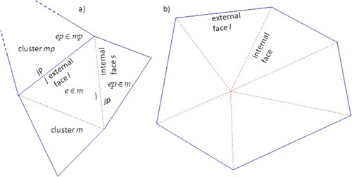
Let us consider irregular a face shared by two tetrahedrons with a negative distance d_e,ep between the corresponding circumcenters, as defined in Equation (25). If one or more irregular faces are present in the mesh, the EDP condition is no longer satisfied (see section 2.2). We group all the tetrahedrons in clusters. A cluster is to be seen as a small non-empty group of neighboring tetrahedrons not sharing any irregular face with other clusters. For example, the two tetrahedrons in Figure 2(b) form a cluster. Each tetrahedron belongs to a single cluster. A single tetrahedron e forms a cluster by itself if it has no irregular faces. In the cluster, we distinguish the external faces, shared by two tetrahedrons of different clusters, and the other internal ones. According to the previous assumptions, all external faces are regular, and in a cluster composed of a single tetrahedron we do not have internal faces.

Let N_C be the number of clusters, with N_C ≤ N_T. The general strategy is to write, instead of the dynamic equilibrium of each single tetrahedron, the dynamic equilibrium of each cluster as a function of a single velocity variation and finally to correct all the tetrahedron velocities inside the clusters, after the CS2 correction step, in order to guarantee flux continuity through all the faces.

From now on, indices m and mp refer to two neighboring clusters, N_T,m is the number of tetrahedrons e belonging to the m-th cluster, $N_{f,m}^{ext}$ and $N_{f,m}^{\mathrm{int}}$ are the number of external and internal faces of the cluster m, l and r are the local counters of the external and internal faces of the cluster, respectively (l = 1, … , $N_{f,m}^{ext}$, r = 1, … , $N_{f,m}^{\mathrm{int}}$), and W_m is the volume of the cluster, $W_m={\sum }_{e=1,N_{T,m}}{W}_e$ (see also Figure 6).

Figure 6. (a) 2D sketch of case $N_{f,m}^{\mathrm{int}}$ = N_T,m – 1. (b) 2D sketch case of $N_{f,m}^{\mathrm{int}}$ = N_T,m. Blue solid lines are traces of the external faces of the cluster, and red dashed lines are traces of the internal faces of the cluster.

4.2. The PS and CS1 problems for non-Delaunay meshes

Solution of the MAST prediction step, as explained in section 3.1, is not affected by the existence of irregular faces. On the other hand, after solution of all tetrahedrons, we need to evaluate, for each cluster, a single velocity variation corresponding to the cluster dynamic equilibrium. Call ${\mathbf{\text{up}}}_e^{k+1/3}\in P_{0,e}$ the predicted tetrahedron velocity computed at time t^k+1/3 as described in section 3.1 for ${\mathbf{\text{u}}}_e^{k+1/3}$ in the case of Delaunay meshes, and $\mathrm{\Delta }{\widetilde{\mathbf{\text{u}}}}_m$ the unknown velocity variation between time levels t^k+1/3 and t^k to be assigned to cluster m.

For each tetrahedron e of cluster m, we can write the correction velocity ${\mathbf{\text{up}}}_e^{k+1/3}-{\mathbf{\text{u}}}_e^k\in P_{0,e}$ by summing the time integrals of the ODEs system (16) and (18), to get (52) $\begin{array}{rl}& ({\mathbf{\text{up}}}_e^{k+1/3}-{\mathbf{\text{u}}}_e^k)W_e\\ & =-\left(\sum _{j=1,4}{\overline{\mathbf{\text{M}}}}_j^{e,out}+\sum _{j=1,4}{\overline{\mathbf{\text{M}}}}_j^{e,in}+{\mathbf{\text{S}}}_{\mathrm{\Psi },e}^k+{\mathbf{\text{FV}}}_e^{k-1/3}\right)\\ & \times \mathrm{\Delta }t\end{array}$(52) where the symbols have been defined in section 3.1. ${\overline{\mathbf{\text{M}}}}_j^{e,out}$ has been computed in the forward step if $R_e^k<R_{ep}^k$ and in the backward step otherwise, ${\overline{\mathbf{\text{M}}}}_j^{e,in}$ has been computed in the forward step if $R_e^k>R_{ep}^k$ and in the backward step otherwise. Observe that, in all internal faces of the cluster, the following condition holds (53) ${\overline{\mathbf{\text{M}}}}_j^{e,out}=-{\overline{\mathbf{\text{M}}}}_{jp}^{ep,in}$(53)

This implies that, summing the Equation (52) of all the tetrahedrons of the same cluster, we get (54) $\begin{array}{rl}& \sum _e({\mathbf{\text{up}}}_e^{k+1/3}-{\mathbf{\text{u}}}_e^k)W_e\\ & =-\sum _e(\sum _{j=1,4}{\overline{\mathbf{\text{M}}}}_j^{e,out}\\ & +\sum _{j=1,4}{\overline{\mathbf{\text{M}}}}_j^{e,in}+{\mathbf{\text{S}}}_{\mathrm{\Psi },e}^k+{\mathbf{\text{FV}}}_e^{k-1/3})\mathrm{\Delta }t\\ & e=1,\dots ,{N_T}_{,m}\end{array}$(54) where all the momentum fluxes belonging to internal faces as well as the corresponding viscous forces, sum zero and can be deleted. Equation (54) can be seen as the equilibrium equation of the cluster m, which can be approximated by setting (55) $\mathrm{\Delta }{\widetilde{\mathbf{\text{u}}}}_m=\frac{\sum _e({\mathbf{\text{up}}}_e^{k+1/3}-{\mathbf{\text{u}}}_e^k)W_e}{W_m}\text{with}\mathrm{\Delta }{\widetilde{\mathbf{\text{u}}}}_m\in P_{0,m}$(55) and by replacing in each tetrahedron the previously computed ${\mathbf{\text{up}}}_e^{k+1/3}$ velocity with (56) ${\mathbf{\text{u}}}_e^{k+1/3}={\mathbf{\text{u}}}_e^k+\mathrm{\Delta }{\widetilde{\mathbf{\text{u}}}}_{m}e=1,\dots ,{N_T}_{,m}$(56)

In the CS1 step, solution of Equation (31) in not EDP meshes is hindered by the negative distances d_e,ep holding between the two circumcenters of tetrahedrons sharing an irregular face. To circumvent the problem, we write the viscous forces equilibrium of the cluster, where the external forces act always on regular external faces. Following the same procedure applied in section 3.2, integrating in space and time Equation (7b) and applying the Green lemma, we get the following system, (57) $\begin{array}{rl}& \sum _{e=1,N_{T,m}}\frac{{\mathbf{\text{u}}}_e^{k+2/3}-{\mathbf{\text{u}}}_e^{k+1/3}}{\Delta t}{W}_e\\ & +\nu \sum _{l=1,N_{f,m}^{ext}}{\sigma }_l^m\frac{{\mathbf{\text{u}}}_e^{k+2/3}-{\mathbf{\text{u}}}_{ep}^{k+2/3}}{d_{e,ep}}\\ & =\nu \sum _{l=1,N_{f,m}^{ext}}{\sigma }_l^m\frac{{\mathbf{\text{u}}}_e^{k+1/3}-{\mathbf{\text{u}}}_{ep}^{k+1/3}}{d_{e,ep}}m=1,\dots ,N_C\end{array}$(57) where ep is the tetrahedron of cluster r, sharing with tetrahedron e the l-th external face of cluster m, with area ${\sigma }_l^m$, distance d_e,ep is defined in Equation (25), and the other symbols have been previously specified.

We set, for the tetrahedrons of cluster m (58) $\begin{array}{rl}{\mathbf{\text{u}}}_e^{k+2/3}& ={\mathbf{\text{u}}}_e^{k+1/3}+\mathrm{\Delta }{\stackrel{⌢}{\mathbf{u}}}_{\mathbf{m}}\\ e& =1,\dots ,{N_T}_{,m}\text{with}\mathrm{\Delta }{\stackrel{⌢}{\mathbf{u}}}_{\mathbf{m}}\in P_{0,m}\end{array}$(58) and, substituting Equations (56) and (58) in Equation (57), we obtain 3 systems, one for each of the unknown components of $\mathrm{\Delta }{\stackrel{⌢}{\mathbf{u}}}_{\mathbf{m}}$, (59) $\begin{array}{rl}& \frac{\mathrm{\Delta }{\stackrel{⌢}{\mathbf{u}}}_m}{\Delta t}{W}_m+\nu \sum _{l=1,N_{f,m}^{ext}}{\sigma }_l^m\frac{\mathrm{\Delta }{\stackrel{⌢}{\mathbf{u}}}_m-\mathrm{\Delta }{\stackrel{⌢}{\mathbf{u}}}_r}{d_{e,ep}}\\ & =\nu \sum _{l=1,N_{f,m}^{ext}}{\sigma }_l^m\frac{\mathrm{\Delta }{\widetilde{\mathbf{\text{u}}}}_m-\mathrm{\Delta }{\widetilde{\mathbf{\text{u}}}}_r}{d_{e,ep}}m=1,\dots ,N_C\end{array}$(59)

Matrix of system (59) has the same properties of matrix of system (31), is symmetric and positive definite, its diagonal and off-diagonal coefficients $M_{e,e}^{C{S}_1}$ and $M_{e,ep}^{C{S}_1}$ are, respectively, (60) $M_{m,m}^{C{S}_1}=\frac{W_m}{\Delta t}+\nu \sum _{l=1,N_{f,m}^{ext}}{\sigma }_l^m\frac{1}{d_{e,ep}},M_{m,r}^{C{S}_1}=-\nu {\sigma }_l^m\frac{1}{d_{e,ep}}$(60) and the m-th coefficient of the source term vector is the r.h.s. of Equation (57). Diagonal and off-diagonal matrix coefficients in Equation (60) are positive and non-positive, respectively, since all the distances d_e,ep are positive.

We deal with the BCs of the CS1 problem as described in section 3.2. Observe that the previously described procedure fails to guarantee in the clusters a positive distance from a boundary element circumcenter and the circumcenter of its boundary face. On the other hand, to guarantee a positive distance from the boundary we can simply avoid any internal node with a distance from the circumcenter of each triangular boundary face smaller than the radius of the circle passing through the three nodes of the same boundary triangle. This can be easily done with a methodology that will be shown in section 5.1.

After solution of system (59), the velocity in the tetrahedrons e of each cluster m is updated according to Equation (58). At time level t^k+2/3 we need to compute for each tetrahedron e the sum ${\mathbf{\text{FV}}}_e^{k+2/3}$ of the viscous forces over its four faces, including the irregular ones, needed for the next computational time step. To do that we assume, coherently with the approximation of Equation (58), the local inertia per unit volume in each tetrahedron, to get (61) $\begin{array}{rl}{\mathbf{\text{FV}}}_e^{k+2/3}& =-\frac{({\mathbf{\text{u}}}_e^{k+1/3}-{\mathbf{\text{u}}}_e^k)}{\mathrm{\Delta }t}{W}_e-{\mathbf{\text{S}}}_{\mathrm{\Psi },e}^k\\ & -\sum _{j=1,4}{\overline{\mathbf{\text{M}}}}_j^{e,out}+\sum _{j=1,4}{\overline{\mathbf{\text{M}}}}_j^{e,in}\end{array}$(61) where the symbols of the momentum fluxes are the same used for the r.h.s of Equation (52).

As it happens for the CS1 problem in the EDP meshes (section 3.2), at time level t^k+2/3, the continuity of the fluxes crossing the same face of two neighboring elements e and ep belonging to two different clusters, is not yet restored, ${\mathbf{\text{u}}}_e^{k+2/3}\in P_{0,e}$, and mass conservation is not satisfied.

4.3. The CS2 problem for non-Delaunay meshes

In non-Delaunay meshes the solution of the CS2 problem is split into two sub-steps. In the first sub-step we apply the procedure described in section 3.3, including in the mass balance the fluxes crossing the external faces of the cluster instead of the fluxes of the four faces of the single tetrahedron (as in Equations (43) and (44)), and assuming a single η value for the circumcenters of all the tetrahedrons inside the cluster. System (44) becomes (62) $\begin{array}{rl}& \mathrm{\Delta }t\sum _{l=1,N_{f,m}^{ext}}{\sigma }_l^e\frac{{\eta }_m-{\eta }_{mp}}{d_{e,ep}}+\sum _{l=1,N_{f,m}^{ext}}({\overline{Fl}}_{l,e}^{k+2/3}-F{l}_{l,e}^k)\\ & =0m=1,\dots ,N_C\end{array}$(62) with the symbols already specified and distance d_e,ep is always positive according to section 4.1. We call ${\overline{Fl}}_{l,e}^{k+2/3}$ the flux crossing face l as defined in Equation (39) over face j (j = 1, … , 4) of e, and $F{l}_{l,e}^k$ the flux due to velocity ${\mathbf{\text{u}}}_e^k\in {\mathbf{\text{X}}}_e$ crossing the same face.

The diagonal and off-diagonal matrix coefficients for system (62a) $M_{m,m}^{C{S}_2}$ and $M_{m,mp}^{C{S}_2}$ are, respectively, (63a) $M_{m,m}^{C{S}_2}=\sum _{l=1,N_{f,m}^{ext}}{\sigma }_l^e\frac{\mathrm{\Delta }t}{d_{e,ep}},M_{m,mp}^{C{S}_2}=-{\sigma }_l^m\frac{\mathrm{\Delta }t}{d_{e,ep}}$(63a) and the same M-property of the coefficients of the matrix of the system of CS1 holds (see section 3.2). The m-th coefficient of the source term vector is (63b) $S{t}_m^{C{S}_2}=-\sum _{l=1,N_{f,m}^{ext}}({\overline{Fl}}_{l,e}^{k+2/3}-F{l}_{l,e}^k)$(63b)

The solution of the system formed by Equations (62)–(63) guarantees flux continuity on the external faces and global mass conservation inside the cluster, but because the velocities ${\mathbf{\text{u}}}_e^{k+1}$ inside each cluster do not generally belong to a single RT0 space, it does not guarantee zero divergence condition inside the cluster, unless the cluster includes only one tetrahedron.

For clusters composed of more than one tetrahedron, we apply the following procedure. We change, in Equation (47), the fluxes $({\overline{Fl}}_{j,e}^{k+2/3}+F{l}_{j,e}^{\eta })$ crossing the internal faces of the cluster, with the unknown flux $F{l}_{j,e}^{\mathrm{int}}$, to get (64) ${\mathbf{\text{u}}}_e^{k+1}=\sum _{j=1,4}{\mathit{\omega }}_j^e[{\tilde{\phi }}_{j}F{l}_{j,e}^{\mathrm{int}}+(1-{\tilde{\phi }}_j)(F{l}_{j,e}^{\eta }+{\overline{Fl}}_{j,e}^{k+2/3})]$(64) where $F{l}_{j,e}^{\mathrm{int}}$ is the flux crossing face j of element e, which is internal to the cluster, and ${\tilde{\phi }}_j$ is 1 if face j is internal to the cluster, and 0 if it is external. We also assume (65) $F{l}_{j,e}^{\mathrm{int}}=-F{l}_{jp,ep}^{\mathrm{int}}$(65) and we look for the optimal set of internal fluxes that: (1) guarantees the condition ${\mathbf{\text{u}}}_e^{k+1}$ $\in P_{0,e}$ for all the elements of the cluster and, as a consequence of constraint (65), mass conservation too, (2) minimizes the kinetic energy inside the cluster.

To get the required $F{l}_{j,e}^{\mathrm{int}}$ fluxes, in the second sub-step of the CS2 problem, for each cluster we solve the following linearly constrained quadratic minimization problem, (66) $\begin{array}{rl}& \text{Minimize }\mathrm{\Im }\\ & =\frac{1}{2}\sum _{e=1,N_{T,m}}\{[\sum _{j=1,4}{\mathit{\omega }}_j^e({\tilde{\phi }}_{j}F{l}_{j,e}^{\mathrm{int}}\\ & +{(1-{\tilde{\phi }}_j)(F{l}_{j,e}^{\eta }+{\overline{Fl}}_{j,e}^{k+2/3}))\phantom{\sum _{j=1,4}}]}^2{W}_e\}\end{array}$(66) subject to Equation (65) and (67) $\begin{array}{rl}& \sum _{j=1,4}({\tilde{\phi }}_{j}F{l}_{j,e}^{\mathrm{int}}+(1-{\tilde{\phi }}_j)(F{l}_{j,e}^{\eta }+{\overline{Fl}}_{j,e}^{k+2/3}))\\ & =0e=1,\dots ,N_{T,m^{-1}}\end{array}$(67) where functional $\mathrm{\Im }$ is the total kinetic energy of the cluster, given by the sum of the kinetic energy of the single tetrahedrons inside it, and the term in the square brackets in Equation (66) is the velocity ${\mathbf{\text{u}}}_e^{k+1}$, according to Equation (64). The last mass conservation Equation (67) in tetrahedron N_T,m has been skipped because solving Equation (62) guarantees global mass conservation inside the cluster and this implies that any Equation (67) can be written as a linear combination of all the other ones. A very efficient way to solve problem (66)-(67) is to compute the Lagrangian multipliers, along with the required unknowns, as the solution of the following unconstrained quadratic minimization problem, (68a) $\begin{array}{rl}& \text{Minimiz}{\text{e}}_{FI,\lambda }\mathrm{\Im }\\ & =\frac{1}{2}\sum _{e=1,N_{T,m}}\{\sum _{j=1,4}[{\mathit{\omega }}_j^e({\tilde{\phi }}_j\sum _{s=1,N_{f,m}^{\mathrm{int}}}{\delta }_{e,j}^{s}F{I}_s\\ & +{(1-{\tilde{\phi }}_j)(F{l}_{j,e}^{\eta }+{\overline{Fl}}_{j,e}^{k+2/3})\phantom{\sum _{s=1,N_{f,m}^{\mathrm{int}}}})]}^2{W}_e\}\\ & +\sum _{e=1,N_{T,m}-1}\{{\lambda }_e\sum _{j=1,4}({\tilde{\phi }}_j\sum _{s=1,N_{f,m}^{\mathrm{int}}}{\delta }_{e,j}^{s}F{I}_s\\ & +(1-{\tilde{\phi }}_j)(F{l}_{j,e}^{\eta }+{\overline{Fl}}_{j,e}^{k+2/3})\phantom{\sum _{s=1,N_{f,m}^{\mathrm{int}}}})\}\end{array}$(68a) where FI_s is the s^th internal flux, occurring between tetrahedrons e and ep of the same cluster m, assumed positive if going from the element with the smallest index to the element with the highest index, and (68b) $\begin{array}{rl}{\delta }_{e,j}^s& =1\text{ if face }s\text{ belongs to element }e\text{ and }e<ep\end{array}$(68b) (68c) $\begin{array}{rl}{\delta }_{e,j}^s& =-1\text{ if face}s\text{ belongs to element }e\text{ and }e>ep\end{array}$(68c) (68d) $\begin{array}{rl}{\delta }_{e,j}^s& =0\text{ if face }s\text{ does not belong to element }e\end{array}$(68d) and $F{l}_{j,e}^{\mathrm{int}}={\delta }_{j,e}^{s}F{I}_s$, if s the index of the face between elements e and ep. The unknowns λ_e are the so-called Lagrangian multipliers. Setting at zero the derivatives of functional $\mathrm{\Im }$ with respect to FI_s and λ_e, we get the linear system (69a) $\begin{array}{rl}& \sum _{e=1,N_{T,m}}\{\sum _{j=1,4}[\sum _{q=1,3}{\omega }_{j,q}^e({\tilde{\phi }}_j\sum _{s=1,.N_{f,m}^{\mathrm{int}}}{\delta }_{e,j}^{s}F{I}_s\\ & +(1-{\tilde{\phi }}_j)(F{l}_{j,e}^{\eta }+{\overline{Fl}}_{j,e}^{k+2/3})\phantom{\sum _{s=1,.N_{f,m}^{\mathrm{int}}}}){\omega }_{j,q}^e]{\tilde{\phi }}_j{\delta }_{e,j}^r{W}_e\}\\ & +\sum _{e=1,N_{T,m}-1}\left\{{\lambda }_e\sum _{j=1,4}({\tilde{\phi }}_j{\delta }_{e,j}^r)\right\}\\ & =0\text{ with }r=1,\dots ,N_{f,m}^{\mathrm{int}}\end{array}$(69a) (69b) $\begin{array}{rl}& \sum _{j=1,4}\left({\tilde{\phi }}_j\sum _{s=1,\dots ,N_{S,m}}{\delta }_{e,j}^{s}F{I}_s+(1-{\tilde{\phi }}_j)(F{l}_{j,e}^{\eta }+{\overline{Fl}}_{j,e}^{k+2/3})\right)\\ & =0\text{for }e=1,\dots ,N_{T,m^{-1}}\end{array}$(69b)

Observe that Equation (69b) represent the mass conservation equations for all the tetrahedrons of cluster m. Moreover, if $N_{f,m}^{\mathrm{int}}$= N_T,m-1 (see the 2D sketch in Figure 6(a)), system (69b) can be solved independently of Equation (69a) and there is only one set of internal fluxes that satisfy the mass conservation equations. If $N_{f,m}^{\mathrm{int}}$≥ N_T,m (see the 2D sketch in Figure 6(b)), we also have to compute Equation (69a) along with Equation (69b), because we need to select, among all the sets of internal fluxes that satisfy mass conservation, the one that minimizes the kinetic energy within the cluster.

Equation system (69) has no special structure and has to be solved with direct solvers, but it is small and only includes a few tetrahedrons of the mesh, so its solution requires a negligible computational burden.

After Equations (64)-(69) are solved, in non-Delaunay meshes we cannot compute the gradient $\mathrm{\nabla }{\mathrm{\Psi }}_e^{k+1}$ of each tetrahedron by applying Equation (48) with the computed ${\mathbf{\text{u}}}_e^{k+1}$ velocity. The reason is that, after the first sub-step of the CS2 problem, the computed solution satisfies the momentum and continuity equations of the clusters (not of the single tetrahedrons) and only the fluxes crossing the external faces of the clusters are computed under these constraints. The fluxes crossing the internal faces of each cluster are computed, during the second sub-step of the CS2 problem, by satisfying the continuity equations only. For these reasons, we compute $\mathrm{\nabla }{\mathrm{\Psi }}_e^{k+1}$ by applying the following general procedure.

We look for a new velocity ${\mathbf{\text{u}}}_m^c$ common to all the tetrahedrons of the cluster. Let ${\mathrm{\Im }}^{\mathrm{\prime }}$ be a scalar functional, defined as (70a) $\begin{array}{rl}{\mathrm{\Im }}^{\mathrm{\prime }}& =\sum _{l=1,N_{f,m}^{ext}}{({\mathbf{\text{u}}}_m^c\cdot {\mathbf{\text{n}}}_l-f{l}_{u,l})}^2\end{array}$(70a) (70b) $\begin{array}{rl}f{l}_{u,l}& =\frac{({\overline{Fl}}_{l,e}^{k+2/3}+F{l}_{l,e}^{\eta })}{{\sigma }_l^m}\end{array}$(70b) where fl_u,l is the flux per unitary area crossing the l-th external face of the cluster, n_l is the unit outward vector normal to face l, and all the other symbols have already been defined. In the case of a cluster made up of a single tetrahedron, according to Equation (47) fl_u,l is the flux per unit area of the velocity ${\mathbf{\text{u}}}_e^{k+1}$ crossing the external l face.

The relationship of ${\mathbf{\text{u}}}_m^c$ with the pressure gradient $\mathrm{\nabla }{\mathrm{\Psi }}_e^{k+1}$ is given by Equation (48), where ${\mathbf{\text{u}}}_e^{k+1}$ is replaced by ${\mathbf{\text{u}}}_m^c$ in the case of N_T,m > 1. Observe that the second step of the CS2 problem does not change the fluxes crossing the external faces and that the pressure gradient $\mathrm{\nabla }{\mathrm{\Psi }}_e^{k+1}$ is not affected by the corrected fluxes of the internal faces. To compute ${\mathbf{\text{u}}}_m^c$ we minimize ${\mathrm{\Im }}^{\mathrm{\prime }}$, which is equivalent to setting at zero the partial derivatives of the functional with respect to the three components of ${\mathbf{\text{u}}}_m^c$. The size of the resulting system is (3 × 3), it does not have a special structure, and, as for system (69), is solved using direct solvers.

Once $\mathrm{\nabla }{\mathrm{\Psi }}_e^{k+1}$ is computed, we obtain the kinematic pressure force on each element of the cluster by setting in all the elements (71) ${\mathbf{\text{S}}}_{\mathrm{\Psi },e}^{k+1}=\mathrm{\nabla }{\mathrm{\Psi }}_e^{k+1}{W}_e$(71) Vector ${\mathbf{\text{S}}}_{\mathrm{\Psi },e}^{k+1}$ is assumed equal to ${\mathbf{\text{S}}}_{\mathrm{\Psi },e}^k$ in the MAST PS of the next time iteration (see Equation (16) in section 3.1).

4.4. The MAST-RT0 pseudo code in the case of non-Delaunay meshes

1. Compute cluster geometry and model constants, including CS1 and CS2 matrix coefficients by means of Equations (60) and (63a). Perform matrix factorization and set k = 1

2. Given u^k and $\mathrm{\nabla }{\mathrm{\Psi }}^k$ at time t^k, apply the MAST prediction step (PS)

   1. Compute velocity variation $\mathrm{\Delta }{\mathbf{\text{u}}}_e^f(\mathrm{\Delta }t)$ and $\mathrm{\Delta }{\mathbf{\text{u}}}_e^b(\mathrm{\Delta }t)$ by solving Equations (16) and (18) for each tetrahedron e

   2. update ${\mathbf{\text{up}}}_e^{k+1/3}={\mathbf{\text{u}}}_e(\mathrm{\Delta }t)$ for each tetrahedron e by means of Equation (18b)

   3. compute one velocity variation $\mathrm{\Delta }{\widetilde{\mathbf{\text{u}}}}_m$ for each cluster m according to Equation (55)

   4. update velocity ${\mathbf{\text{u}}}_e^{k+1/3}$ for each tetrahedron e of each cluster m by means of Equation (56)

3. Apply the 1st corrective step (CS1)

   1. Solve system (59) for the $\mathrm{\Delta }{\stackrel{⌢}{\mathbf{u}}}_{\mathbf{m}}$ unknown for each cluster m

   2. update velocity ${\mathbf{\text{u}}}_e^{k+2/3}$ for each tetrahedron e of each cluster m by means of Equation (58)

4. Update the viscous forces ${\mathbf{\text{FV}}}_e^{k+2/3}$ for each tetrahedron e by means of Equation (61)

5. Compute fluxes ${\overline{Fl}}_{l,e}^{k+2/3}({\mathbf{\text{u}}}^{k+2/3})$ for each external face l of tetrahedron e of each cluster m, by means of Equation (39)

6. Apply the 2^nd corrective step (CS2)

   1. Compute η_m for each cluster m by solving system (62)

   2. Compute the fluxes $F{l}_{j,e}^{\mathrm{int}}$ of the internal faces j of tetrahedrons e of the cluster m according to Equations (66)-(69)

   3. Compute fluxes $F{l}_{j,e}^{\eta }$ of the cluster external faces by means of Equation (46)

   4. Update the final velocity ${\mathbf{\text{u}}}_e^{k+1}$ for each tetrahedron e according to Equation (64)

   5. Compute ${\mathbf{\text{u}}}_m^c$ by solving the minimization problem in Equations (70)

7. Update the gradient of the kinematic pressure $\mathrm{\nabla }{\mathrm{\Psi }}^{k+1}$ according to Equation (48), where ${\mathbf{\text{u}}}_e^{k+1}$ is replaced by ${\mathbf{\text{u}}}_m^c$

8. Compute the kinematic pressure forces ${\mathbf{\text{S}}}_{\mathrm{\Psi },e}^{k+1}$ for each tetrahedron e by means of Equations (70)–(71)

9. Set k = k+1 and go to point 2 for the solution of the next time step.

5. Model applications

5.1. Construction of the computational mesh and preliminary model operations

As mentioned in section 3.3, in the 3D space it is almost impossible to obtain a mesh satisfying the EDP given in Equations (10)–(11) (Forsyth, 1991; Joe, 1986 and cited references). Some algorithms exist (e.g. Qhull in Matlab³), which generate a 3D tetrahedral mesh forming a convex hull with arbitrary node location. Unfortunately, the generated mesh has very irregular elements inside it (e.g. slivers, caps, skinny tetrahedrons, …), along with several distances d_e,ep (see Equation (25)) strictly equal or close to zero. These irregularities always lead to instability and poor accuracy of the numerical solution (Letniowski, 1992).

The computational mesh used by the present solver is created by an off-line procedure, using two open source mesh generators, Netgen (Schöberl, 1997) and Tetgen (Hang, 2015).

We discretize first the computational domain with tetrahedrons using the mesh generator Netgen. The tetrahedral elements of the output mesh are quite regular in shape and size, even if they do not satisfy the EDP. Netgen also allows us to change the size of the tetrahedrons to discretize the internal subdomains properly, with quite smooth transitions of element size. Netgen also allows ‘user-friendly’ handling of the boundary domain.

Let N_NET be the number of nodes of the Netgen mesh. For each boundary triangle bt we compute the corresponding circumsphere Σ_bt whose diametral plane contains bt, and we check if any internal node (i.e. not belonging to boundary faces) is internal to Σ_bt. At the end of this operation, we remove all the internal nodes inside the circumsphere of the boundary triangles (usually 0.02-0.03% of N_NET). We call the number of the removed nodes N_r. The ensemble of the (N_NET – N_r) nodes is the input for the mesh generator TETGEN, which regenerates the mesh domain starting from the nodal positions of the (N_NET – N_r) nodes, still preserving the input domain boundaries. In order to optimize some aspect-ratio and shape tetrahedrons conditions, Tetgen can also insert additional Steiner nodes (Hang, 2015). The present numerical solver uses as its input the Tetgen output mesh.

Preliminary model operations concern (1) generation of the topology of the tetrahedrons and clusters of tetrahedrons, saved in separate arrays, (2) calculation of the matrix coefficients of systems (59)–(60) and (62), and (3) their factorization before the time iterations loop start.

5.2. Computation of the kinematic pressure ψ and of the body forces

Let N be the number of nodes of the computational mesh. We approximate the function ψ according to a Galerkin Finite Element approach, (72) $\mathrm{\Psi }=\sum _{i=1,N}{w}_i{\tilde{\mathrm{\Psi }}}_i$(72) where ${\tilde{\mathrm{\Psi }}}_i$ is the unknown nodal pressure value and w_i is the Galerkin shape function in node i. Once $\mathrm{\nabla }{\mathrm{\Psi }}_e^{k+1}$ has been obtained inside each tetrahedron e as specified in sections 3.3 and 4.3, we minimize the following scalar functional, (73a) ${\mathrm{\Im }}_{\mathrm{\Psi }}=\sum _{e=1,N_T}{(\mathrm{\nabla }{\tilde{\mathrm{\Psi }}}_e^{k+1}-\mathrm{\nabla }{\mathrm{\Psi }}_e^{k+1})}^2$(73a) rewritten as (73b) $\begin{array}{rl}& {\mathrm{\Im }}_{\mathrm{\Psi }}=\sum _{e=1,N_T}\left[\sum _{q=1,3}\left\{\sum _{i=1,N}{\left(\frac{\mathrm{\partial }{w}_i}{\mathrm{\partial }{x}_q}{\tilde{\mathrm{\Psi }}}_i-{({\mathrm{\nabla }}_{x_q}{\mathrm{\Psi }}^{k+1})}_e\right)}^2\right\}\right]\\ & q=\{\begin{array}{c}1\\ 2\\ 3\end{array}\Rightarrow x_q=\{\begin{array}{c}x\\ y\\ z\end{array}\end{array}$(73b) where $({\mathrm{\nabla }}_{x_q}{\mathrm{\Psi }}^{k+1}{)}_e$ is the q-th components of $\mathrm{\nabla }{\mathrm{\Psi }}^{k+1}$ in tetrahedron e, previously computed. ${\mathrm{\Im }}_{\mathrm{\Psi }}$ is a convex function and its minimum is obtained by setting at zero the partial derivatives of Equation (73b) with respect to the nodal ${\tilde{\mathrm{\Psi }}}_i^{k+1}$ values, (74a) $\frac{\mathrm{\partial }{\mathrm{\Im }}_{\mathrm{\Psi }}}{\mathrm{\partial }{\mathrm{\Psi }}_i^{k+1}}=0i=1,\dots ,N$(74a)

Equation (74a) can be written, according to Equation (72), as (74b) $\begin{array}{rl}\frac{\mathrm{\partial }{\mathrm{\Im }}_{\mathrm{\Psi }}}{\mathrm{\partial }{\tilde{\mathrm{\Psi }}}_i^{k+1}}& =\sum _{e=1,N_T}[\sum _{q=1,3}\{\sum _{l=1,N}(-\frac{\mathrm{\partial }{w}_i}{\mathrm{\partial }{x}_q}{\tilde{\mathrm{\Psi }}}_l\\ & -{({\mathrm{\nabla }}_{x_q}{\mathrm{\Psi }}^{k+1})}_e\phantom{\frac{\mathrm{\partial }{w}_i}{\mathrm{\partial }{x}_q}})\frac{\mathrm{\partial }{w}_i}{\mathrm{\partial }{x}_q}\phantom{\sum _{l=1,N}}\}]=0\end{array}$(74b)

Equation (74b) represents a linear system solved for the ${\tilde{\mathrm{\Psi }}}_l$ unknowns, with an (N x N) system matrix that is sparse, symmetric and positive-definite. Over the boundary faces of Γ_σ, we assign Dirichlet BCs for ${\tilde{\mathrm{\Psi }}}_l$ according to the prescribed boundary values. The diagonal and off-diagonal coefficients are (75a) $M_{i,i}^{\mathrm{\Psi }}=\sum _{q=1,3}\frac{\mathrm{\partial }{w}_i}{\mathrm{\partial }{x}_q}\frac{\mathrm{\partial }{w}_i}{\mathrm{\partial }{x}_q},M_{i,l}^{\mathrm{\Psi }}=\sum _{q=1,3}\frac{\mathrm{\partial }{w}_i}{\mathrm{\partial }{x}_q}\frac{\mathrm{\partial }{w}_l}{\mathrm{\partial }{x}_q}$(75a) and the i-th coefficient of the source term vector is (75b) $S_i^{\mathrm{\Psi }}=-({\mathrm{\nabla }}_{x_q}{\mathrm{\Psi }}^{k+1}{)}_e\frac{\mathrm{\partial }{w}_i}{\mathrm{\partial }{x}_q}$(75b)

We solve system (74)–(75) as the previous ones in sections 3.2, 3.3, or 4.2 and 4.3.

The forces over the bodies are easily computed as, (76a) $\begin{array}{rl}\mathbf{\text{F}}& ={\mathbf{\text{F}}}_{\mathrm{\Psi }}+{\mathbf{\text{F}}}_{\nu }\text{ with }{\mathbf{\text{F}}}_{\mathrm{\Psi }}\\ & =\sum _{b=1,N_{bf}}\left({\sigma }_b\frac{\left(\sum _{f_b=1,2,3}{\tilde{\mathrm{\Psi }}}_{f_b}\right){\mathbf{\text{n}}}_b}{3}\right)\end{array}$(76a) and (76b) $\begin{array}{rl}{\mathbf{\text{F}}}_{\nu }& =\sum _{b=1,N_{bf}}\left(\nu \frac{({\mathbf{\text{u}}}_e^{k+1}-{\mathbf{\text{g}}}_b)}{d_j^e}{\sigma }_b\right)\text{ if }b\in {\mathrm{\Gamma }}_u\end{array}$(76b) (76c) $\begin{array}{rl}{\mathbf{\text{F}}}_{\nu }& =0\text{ if }b\in {\mathrm{\Gamma }}_{\sigma }\vee {\mathrm{\Gamma }}_m\end{array}$(76c) where N_bf is the number of triangular faces of the body, σ_b and n_b are the area of the b-th body face and the unit normal vector coming into the body, respectively, ${\tilde{\mathrm{\Psi }}}_{f_b}$ is the value of the kinematic pressure at f_b-th node of the body face, g_b is the velocity vector assigned to the face, ${\mathbf{\text{u}}}_e^{k+1}$ is the velocity vector in the tetrahedron e with the b-th body face, and $d_j^e$ is the distance between the circumcenter of tetrahedron e and the circumcenter of the body face, computed as in Equation (33).

5.3. Test cases

The proposed numerical solver was applied to four different numerical tests. In the first test we analyzed the spatial and temporal accuracy of the model, as well as the required computational costs. In tests 2 and 3 we present two well-known literature applications, the lid driven cavity and the flow past a fixed sphere, according to different values of the Reynolds number. In the last test the real case of hemodynamic blood flow inside an abdominal aorta affected by an aneurysm is solved by the model inside a very irregular boundary.

For post-processing of the model outputs, we used the open source program Paraview.⁴

5.3.1. Taylor-Green vortices test

We first analyzed the accuracy of the proposed solver by comparison of the computed results with the known analytical solution of the Taylor–Green vortex test (Taylor & Green, 1937). The velocity vector components and the pressure field are (Taylor & Green, 1937), (77) $\begin{array}{rl}& u=\cos (\alpha x)\sin (\alpha y)e^{-\beta t}\\ & v=-\sin (\alpha x)\cos (\alpha y)e^{-\beta t}w=0\\ & p=-\frac{\cos (2\alpha x)+\cos (2\alpha y)}{4}{e}^{-2\beta t}\\ & a=\frac{\pi }{2}\text{, }\beta =2\nu a^2\text{, }\nu =0.01\frac{m^2}{s}\end{array}$(77) such that the r.h.s. of Equation (1) is always zero. The initial conditions are found by setting t = 0 in Equation (77). We solve this problem up to 2 s in the domain [−3, 3]² x [0, 0.25], by setting time-dependent essential BCs for the velocity, according to Equation (77), in the circumcenters of the boundary triangular faces of the lateral walls of the domain (Γ_u in section 2.1), as well as the hydrostatic stress in the nodes of the upper and lower wall (Γ_σ in section 2.1). The initial velocity vectors are set in the circumcenters of each tetrahedron, and assumed piecewise constant, while the initial kinematic pressures are set in the nodes. The initial values of the forces ${\mathbf{\text{S}}}_{\mathrm{\Psi },e}^0$ and ${\mathbf{\text{VF}}}_e^0$ of the momentum equations of the MAST PS of the first time iteration are analytically found as (78a) $\begin{array}{rl}{\mathbf{\text{S}}}_{\mathrm{\Psi },e}^0& =\mathrm{\nabla }{\mathrm{\Psi }}_e^0{W}_e\end{array}$(78a) (78b) $\begin{array}{rl}{\mathbf{\text{VF}}}_e^0& =\nu {\Delta }_2{\mathbf{\text{u}}}_e^0{W}_e\end{array}$(78b) where $\mathrm{\nabla }{\mathrm{\Psi }}_e^0$ is computed from Equation (77) in the center of mass of tetrahedron e.

We discretize the domain using 5 meshes with mean element characteristic size h_l (l = 1, … , 5) ranging from 0.00996 m to 0.066 m. h_l is the mean value of the length of the sides of the tetrahedrons.

The discretized ICs ${\mathbf{\text{u}}}_e^k={\mathbf{\text{u}}}_{e,0}$ do not satisfy the momentum and continuity equations of each element at time t = 0, as ${\mathbf{\text{u}}}_{e,0}\in$ P_0,e, but the flux continuity through each face is missing. In order to circumvent this problem, before the beginning of the transient flow simulation with the BCs given by Equation (77), we compute the steady-state asymptotic solution corresponding to the BCs at t = 0 and we use it as ICs of the transient problem. We assume that the steady-state solution is attained when the L₂ norm of the relative scatters of the computed u, v, w, and ψ, compared with the ones of the previous iteration, are small and the following tolerance holds (79) $\begin{array}{rl}& \sqrt{\sum _{e=1,N_T}{\left(\frac{u(v,w{)}_e^{k+1}-u(v,w{)}_e^k}{u(v,w{)}_e^k}\right)}^2}\\ & <1e-04\text{.and}\text{. }\sqrt{\sum _{i=1,N}{\left(\frac{{\mathrm{\Psi }}_i^{k+1}-{\mathrm{\Psi }}_i^k}{{\mathrm{\Psi }}_i^k}\right)}^2}<1e-04\end{array}$(79) See in Tables 1 and 2 the L₂ and $L_{\mathrm{\infty }}$ norms of the relative errors of the steady-state x and y velocity components and kinematic pressure with respect to the values computed at the face circumcenters according to Equation (77), for meshes with different size. The error of the z velocity component is negligible compared to the x and y errors.

Table 1. Test 1. L₂ norms of relative errors and spatial rate of convergence.

hl [m]	L2 err u	L2 err v	L2 err ψ	rc,s u	rc,s v	rc,s ψ
6.60E–02	1.36E–02	1.37E–02	2.58E–02	–	–	–
2.47E–02	4.45E–03	4.47E–03	6.24E–03	1.14E+00	1.14E+00	1.45E+00
1.69E–02	2.82E–03	2.84E–03	3.50E–03	1.19E+00	1.18E+00	1.50E+00
1.28E–02	2.03E–03	2.05E–03	2.28E–03	1.18E+00	1.17E+00	1.55E+00
9.96E–03	1.50E–03	1.51E–03	1.53E–03	1.22E+00	1.21E+00	1.59E+00

Table 2. Test 1. L∞ norms of relative errors and spatial rate of convergence.

hl [m]	L∞ err u	L∞ err v	L∞ err ψ	rc,s u	rc,s v	rc,s ψ
6.60E–02	3.04E–02	3.07E–02	5.77E–02	–	–	–
2.47E–02	9.98E–03	1.00E–02	1.40E–02	1.13E+00	1.14E+00	1.44E+00
1.69E–02	6.32E–03	6.35E–03	7.85E–03	1.19E+00	1.18E+00	1.50E+00
1.28E–02	4.56E–03	4.59E–03	5.10E–03	1.18E+00	1.17E+00	1.55E+00
9.96E–03	3.37E–03	3.39E–03	3.44E–03	1.22E+00	1.21E+00	1.59E+00

We also assume that the relative error err_l, computed for the mesh with mean element size h_l, is proportional to a power of h_l, (80a) $er{r}_l=(h_l{)}^{r_{c,s}}$(80a) where r_c,s is the spatial rate of convergence, obtained by comparing the relative errors of two sequential sizes h_l and h_l+1 as (80b) $r_{c,s}=\frac{\log \left(\frac{L_{2}er{r}_l}{L_{2}er{r}_{l+1}}\right)}{\log \left(\frac{h_l}{h_{l+1}}\right)}$(80b)

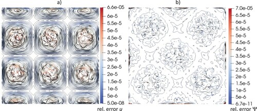
The rate of convergence is shown in Tables 1 and 2. The computed r_c,s of the velocity components are slightly greater than 1 (ranging from 1.14–1.22) due to the piecewise approximation of u and v inside each tetrahedron. The convergence rate obtained for the kinematic pressure is greater (ranging from 1.45–1.59) and the reason could be the nodal pressure distribution inside each tetrahedron, as described in section 5.2. In Figure 7 we plot the iso-contour lines, over a horizontal plane with z = 0.125 m, of the relative errors of the norm of u and of ψ obtained for the coarsest mesh. Close to the lateral boundary walls, the errors of the velocity decrease, due to the imposed BCs. On the opposite, the highest values of the relative errors of the kinematic pressure are close to the boundary lateral walls, since the Dirichlet BCs of ψ have been imposed over the upper and lower horizontal walls.

Figure 7. Test 1. Iso-contours of the relative error of the norm of (a) u, (b) ψ.

In Figure 8(a) we plot the norms of the relative errors, along with the 1st order convergence line.

Figure 8. Test 1. Investigation of the spatial and temporal accuracy. (a) Norms of relative errors vs. mean mesh size, (b) norms of relative errors vs. time step size.

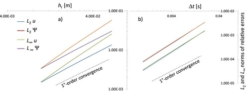
With this test we also analyzed the time convergence rate of the algorithm. In order to cancel out the error due to the spatial discretization, we assumed as the reference solution the one obtained over the finest mesh (with mean size h_l = 0.00996 m), and a time step size Δt = 0.001 s. At simulation time 2 s, we compared with the reference solution the numerical solutions obtained over the same mesh, assuming five different Δt values, ranging from 0.0015 s to 0.02 s. The L₂ and $L_{\mathrm{\infty }}$ norms of the relative errors are shown in Tables 3 and 4, along with the time rate of convergence, r_c,t, computed by comparing the relative errors of two sequential time step sizes Δt_l and Δt_l+1 (80c) $r_{c,t}=\frac{\log \left(\frac{L_{2}er{r}_l}{L_{2}er{r}_{l+1}}\right)}{\log \left(\frac{\mathrm{\Delta }{t}_l}{\mathrm{\Delta }{t}_{l+1}}\right)}$(80c)

Table 3. Test 1. L₂ norms of relative errors and time rate of convergence.

Δt [s]	L2 err u	L2 err v	L2 err ψ	rc,t u	rc,t v	rc,t ψ
0.02	1.50E–03	1.51E–03	1.53E–03	–	–	–
0.015	1.06E–03	1.06E–03	1.07E–03	1.20E+00	1.22E+00	1.26E+00
0.01	6.33E–04	6.33E–04	6.47E–04	1.28E+00	1.28E+00	1.24E+00
0.005	2.60E–04	2.61E–04	2.74E–04	1.28E+00	1.28E+00	1.24E+00
0.0025	1.08E–04	1.08E–04	1.16E–04	1.26E+00	1.27E+00	1.25E+00
0.001	3.39E–05	3.45E–05	3.63E–05	1.27E+00	1.25E+00	1.27E+00

Table 4. Test 1. L∞ norms of relative errors and time rate of convergence.

Δt [s]	$L_{\mathrm{\infty }}$ err u	$L_{\mathrm{\infty }}$ err v	$L_{\mathrm{\infty }}$ err ψ	rc,t u	rc,t v	rc,t ψ
0.02	3.37E–03	3.39E–03	3.44E–03	–	–	–
0.015	2.39E–03	2.38E–03	2.39E–03	1.19E+00	1.22E+00	1.26E+00
0.01	1.42E–03	1.42E–03	1.45E–03	1.29E+00	1.28E+00	1.24E+00
0.005	5.83E–04	5.84E–04	6.15E–04	1.28E+00	1.28E+00	1.24E+00
0.0025	2.44E–04	2.43E–04	2.59E–04	1.26E+00	1.27E+00	1.25E+00
0.001	7.62E–05	7.73E–05	8.12E–05	1.27E+00	1.25E+00	1.27E+00

The rate of convergence r_c,t is always greater than 1, ranging from 1.21–1.28, even if the model is 1st order accurate in time. This could be due to a twofold reason related to the MAST-PS, (1) the use of the internal time sub-grid during the ODEs solution, and (2) a polynomial time approximation order of the leaving momentum fluxes, using n_G = 3 Gauss points. In Figure 8(b) we plot the norms of the relative errors along with the 1st-order convergence line.

For the finest mesh, for each time step adopted for the time convergence rate analysis, we computed the maximum CFL number, as (81) $\text{CF}{\text{L}}_{max}=max\left(\frac{\mathrm{\Delta }t}{\sqrt[3]{W_e}}||{\mathbf{\text{u}}}_e||\right)e=1,\dots ,N_T$(81) CFL_max ranges from 2.56 (for Δt = 0.02) to 0.0128 (for the reference solution).

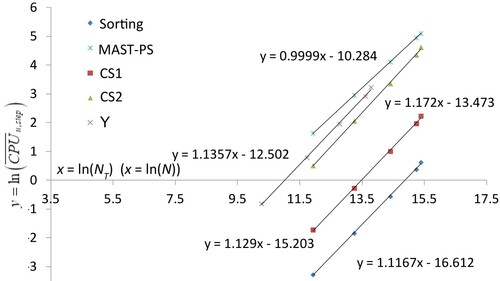
We also investigated the computational (CPU) times required by the different model steps, using a single Intel Core i7 at 3.49 GHz. Because computational times strongly depends on the adopted computer and on the specific algorithm coding, we focused on the correlation existing between the the computational time of the single step and the number of elements. We set the average CPU time per iteration and per model step equal to (82a) ${\overline{CPU}}_{step}=\exp (c){N_T}^{\beta }$(82a) and we assumed that a single step is efficiently solved as much as the β power exponent in the correlation 82(a) is small and close to 1. Equation (82a) in logarithmic space becomes (82b) $\ln ({\overline{CPU}}_{step})=c+\beta \ln (N_T)$(82b)

See in Figure 9 the ${\overline{CPU}}_{step}$ time required for the solution of the single model steps, i.e. cell sorting (${\overline{CPU}}_S$), solution of the MAST-PS step (${\overline{CPU}}_{MPS}$), solution of the CS1 and CS2 steps (${\overline{CPU}}_{CS1}$ and ${\overline{CPU}}_{CS2}$, respectively), as well as the kinematic pressure computation (${\overline{CPU}}_{\mathrm{\Psi }}$). MAST-PS is the most demanding one, but in this case the CPU is simply proportional to N_T, and in Equation (82a) power β is equal to one. The CPU required by the other model steps grows in the logarithm space more than linearly with the number of tetrahedrons due to their ‘non-explicit nature’, since solution of large linear systems is involved, but β is smaller than 1.20 for the CS2 step, and smaller than 1.12 in all the other ones. The sorting cell operation is the least demanding algorithm step and its CPU time is 2–3 magnitude orders smaller than the MAST-PS one.

Figure 9. Test 1. Computational time of model steps.

5.3.2. Lid driven cavity flow at different Reynolds numbers

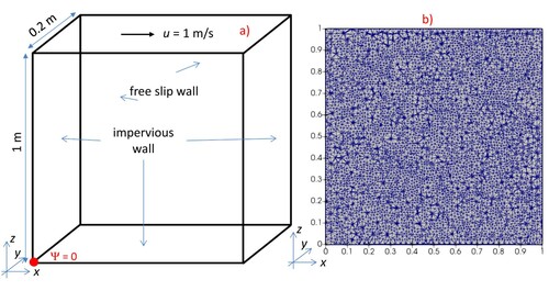
In this test the flow is confined inside a square cavity, and it is driven by the upper wall displacement in horizontal direction. The set-up of the test is shown in Figure 10(a). Cavity is [0, L] x [0, 0.2] x [0, L] with L = 1 m. At the east, west and bottom walls we set zero velocity with no slip BCs (Γ_u), while at the front and rear walls we set free slip BCs (Γ_m), and we impose a constant in time horizontal velocity equal to 1 m/s over the top wall with no slip BCs (Γ_u). We set zero kinematic pressure in the lowest left corner with coordinates (0, 0, 0), as shown in Figure 10(a). ICs are zero velocity and pressure inside domain.

Figure 10. Test 2. (a) set-up of the numerical test and BCs. (b) section of the mesh with a cutting plane.

Let the Reynolds number be (83) $Re=\frac{v_{max}L}{\nu }$(83) where v_max = 1 m/s. We run simulations for Re = 100, 400 and 1000.

The imposed horizontal velocity of the upper lid drives the fluid inside the cavity into a vortical flow. The resulting complex flow structure shows a large central vortex and small recirculating zones close to the cavity corners, whose shape depends on the value of Re.

We discretize the domain with 87,740 tetrahedrons and 17,388 nodes (see in Figure 10(b) an intersection of the mesh with a cutting plane), resulting in 84,385 clusters. The time step size Δt is set to 0.025 s, and the maximum computed CFL values are 2.18, 2.08 and 1.96 for Re = 100, 400 ad 1000, respectively.

In Figure 11 we plot the streamlines, as well as the vorticity and the iso-pressure fields. The minimum and maximum pressures are computed respectively at the upper-left and upper-right corners, where a discontinuity in the boundary condition occurs. Observe that, because of this singularity, no ad-hoc handling is required in the model, unlike what is found in Botella and Peyret (1998), Boppana and Gajjar (2010), Kuhlmann and Romanò (2019), and cited references. The minimum pressure values are associated with the foci of the vortices, due to the high centrifugal acceleration occurring around them. We obtain good agreement with the literature results (e.g. Dalal et al., 2008 and cited references), and the results provided by the present solver match very well the ones of the 2D benchmark solutions given by Ghia et al. (1982) and shown in Figure 12. The results in Figures 11 and 12 refer to the cutting plane (x-z) with y = 0.1 m (i.e. the diametral plane of the domain). The results obtained for other cutting planes (x-z) are very similar to the previous ones, and for brevity are not shown here.

Figure 11. Test 2. Velocity streamlines (left panels), vorticity (ω_z) (central panels), iso (kinematic) pressure (right panels). Top Re = 100, middle Re = 400, bottom Re = 1000.

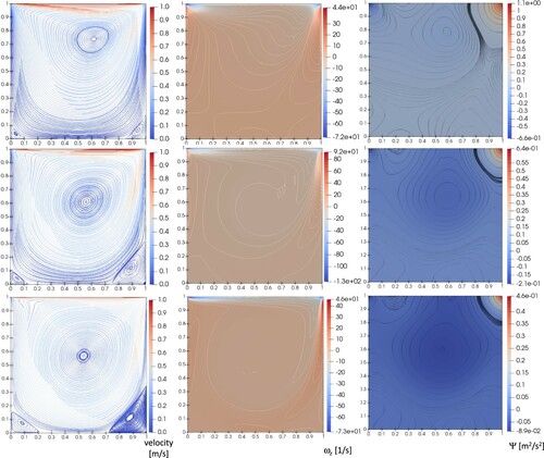
Figure 12. Test 2. x velocity component (top panel), z velocity component (bottom panel) (Nomenclature ‘Ref.’ are the results by Ghia et al. 1982).

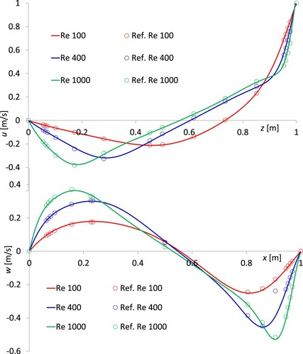
Observe that the value of the vertical velocity component computed for Re = 400 and x = 0.9063 provided by Ghia et al. (1982) (w_Ghia = −0.23827) (see table 2 of the referred paper) is quite different from the result obtained by the present solver. On the other hand, the w_Ghia result is missing in most of the papers where the lid-driven test is used as bench mark, including the papers reporting the solution by Ghia et al. (1982) for many other points (e.g. Xue & Burton, 2013 and many others), whereas in other papers the mentioned w_Ghia vertical velocity component does not match the result, like in Dalal et al. (2008).

5.3.3. Flow past a stationary sphere at different Reynolds numbers

In the past few decades, a plethora of experimental, theoretical and numerical studies of viscous flow past a stationary sphere S have been presented to investigate wake structures. The Reynolds number, defined as (84) $Re=\frac{U_0{D}_s}{\nu }$(84) based on the uniform undisturbed flow velocity U₀, on the diameter of the sphere D_s, and on the surrounding fluid viscosity ν, is used as a parameter to classify the wake structure (e.g. Johnson & Patel, 1999; Ploumhans et al., 2002; Sakamoto & Haniu, 1990, and cited references). The wake structure has been a strongly debated topic, and several controversial findings have been obtained by authors in the literature studies (e.g. Johnson & Patel, 1999; Ploumhans et al., 2002; Sakamoto & Haniu, 1990, and cited references). According to experimental and numerical studies, above 270 < Re < 290, the flow becomes unsteady but periodic, and vortex shedding starts around Re = 300 (e.g. Johnson & Patel, 1999; Ploumhans et al., 2002; Sakamoto & Haniu, 1990, and cited references), with formation of hairpin vortices (as shown in Figure 13, from the experimental studies by Sakamoto and Haniu (1990)). By progressively increasing Re, the vortices start to intertwine with each other, and above Re = 500 periodicity is lost (e.g. Johnson & Patel, 1999; Ploumhans et al., 2002; Sakamoto & Haniu, 1990, and cited references). For a more comprehensive review, we refer the readers to the cited works.

Figure 13. Test 3. Pattern of vortex shedding. Left panels Re = 300, (a) side view, (b) upper view. Right panel (c) 480 < Re < 800 (from Sakamoto & Haniu 1990)).

In the research referred to here we investigated the flow structures around a stationary sphere for Re = 300 and 600. The fluid is assumed to be water. In Figure 14 we plot the 3D view of the domain and the setup of the numerical test. We assume the sphere S, with D_s = 0.0254 m, symmetrically placed inside a large cylinder C with diameter D_C = 0.3 m ($\simeq$ 12 D_s) and length 1.1 m ($\simeq$ 43.5 D_s). The center of S is located 0.15 m ($\simeq$ 6 D_s) downstream of the inflow upstream face of C. At the upstream inflow section of C we set u uniform and constant in time (U₀, 0, 0), and the same velocity is imposed at the lateral walls of C in such a way that the flow around S is only weakly affected by the walls. Zero pressure is assumed at the downstream outflow section. Over the surface of S we assume no-slip BC. We assume flow at rest and zero pressure inside C at t = 0.

Figure 14. Test 3. (a) 3D view of the domain. (b) setup and BCs of the numerical runs.

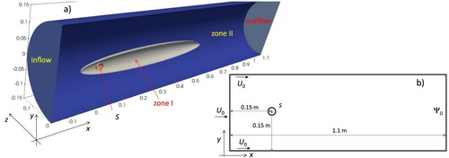
The mesh size is refined in zone I (around S and downstream of it, as shown in Figure 14(a)) in order to reproduce the strong velocity gradients close to the surface of S and the fluid vortices in the wake. A larger mesh size is adopted for the rest of the domain (zone II in Figure 14(a)). The mesh size (defined as in test 1) used for zones I and II is 0.00055 and 0.0128 m, respectively, with a smooth transition between the two zones. The total number of tetrahedrons in the mesh is 2,309,771, with 2,243,199 clusters and 392,850 nodes, and the surface of S is discretized with 4332 triangles.

Unfortunately, description of initiation of vortex shedding is most often ignored in numerical studies. In physical experiments, initiation of vortex shedding is generated by flow instabilities amplifying small flow disturbances (Sungsu, 2000). Such disturbances include, among others, asymmetric domain geometry, vibrations of the pipe, non-uniformity and turbulence of the inflow velocity, non-uniform roughness of the pipe walls and sphere surface, … (Sungsu, 2000). All these sources are missing in numerical experiments, and, for a stationary sphere inside a symmetric domain, symmetric steady solution are attained even for Reynolds numbers at which experimental unsteady vortex shedding has been detected (Sungsu, 2000). In numerical experiments, vortex shedding could be generated by (1) computational truncation and round-off errors, strongly dependent on the characteristics of the numerical solver and the computer, or (2) specifically introduced numerical perturbations (Sungsu, 2000). Examples of such numerical perturbations can be found, for example, in Ploumhans et al. (2002), Sungsu (2000) and cited references.

We performed a first series of simulations at Re = 300 without numerical perturbations, with an impulsive start of the inflow velocity. After rapid changes during the early stages of the process, the flow characteristics converted to a stationary solution. In Figure 15 we plot the streamlines of the stationary flow field in the (x-y) plane. After the early transient process due to the impulsive flow start, we computed the stationary values of drag and lift coefficients C_D and C_L listed in Table 5. These were obtained as $C_D=F_x/(1/2\rho U_0\pi D_S^2/4)$ and $C_L=F_y/(1/2\rho U_0\pi D_S^2/4)$, where F_x and F_y are the x and y components of the total force, sum of the pressure and the viscous forces. The streamlines in the (x-z) plane are almost symmetrical, and the mean-in-time value of the side coefficient C_S, obtained as $C_S=F_z/(1/2\rho U_0\pi D_S^2/4)$, is 1.34e-05.

Figure 15. Test 3, Re = 300. Velocity streamlines in the (x–y) plane, stationary case.

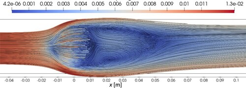
Table 5. Test 3. Values of the drag and lift coefficients.

	CD [–]		CL [–]
	Mean value	Amplitude value	Mean value	Amplitude value
Present solver without perturbation	0.67043	–	−0.0675	–
Present solver with perturbation (Equation (85))	0.6678	2.91E-03	−0.06061	1.47E-02
Ploumhans et al. (2002)	0.683	2.50E-03	−0.061	1.40E-02
Johnson and Patel (1999)	0.656	3.50E-03	−0.069	1.60E-02
Tomboulides (1993)	0.671	2.80E-03	not reported	not reported
Roos and Willmarth (1971)	0.629	not reported	not reported	not reported

It is important to underline that C_D and C_L are in very good agreement with the mean in time values provided by literature studies, which are reported in Table 5.

Similarly to Ploumhans et al. (2002), the most efficient method for the present solver to trigger vortices has been, after the impulsive flow start, to set the y velocity component (85) $v=\sin (\pi (\tau \ast -3))\frac{U_0}{4}\text{ with }\tau \ast =t{U}_0/D_S$(85) in the interval $3\le \tau \ast \le 4$, along the inflow section and the lateral walls of C. The time step size used for the simulations is 0.05 s and the maximum computed value of the CFL number is 3.5.

In Figure 16 we plot the 3D view of the vorticity structures identified by the Q-criterium (Hunt et al., 1988). In Figures 17 and 18 we show the velocity streamlines and the iso-contour lines of the kinematic pressure in the (x-y) and (x-z) planes, respectively. The time difference among the panels is one quarter of a period, and after the fourth panel (3/4 of period), the cycle repeats again. The present model satisfactorily reproduces the hairpin shapes of the vortical structure. Observe that, due to the strong pressure gradients feeding the movement of the vortices, the pressure minima in this case do not match their foci.

Figure 16. Test 3, Re = 300. 3D periodic time evolution of the vortical structures.

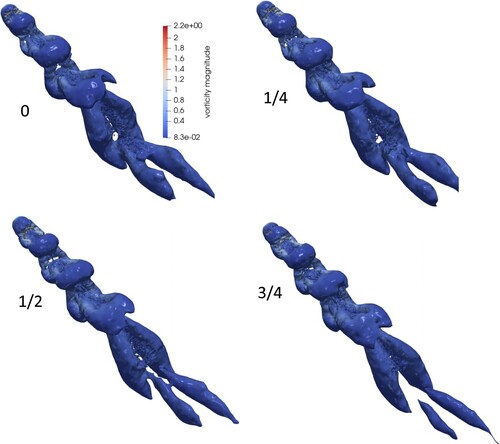
Figure 17. Test 3, Re = 300. Periodic time evolution of the velocity streamlines (left panels) and kinematic pressure (right panels), (x–z) plane.

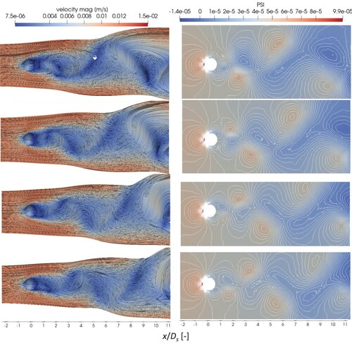
Figure 18. Test 3, Re = 300. Periodic time evolution of the velocity streamlines (left panels) and kinematic pressure (right panels), (x–y) plane.

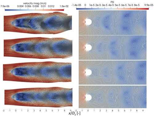
After a rapid transient phase, due to the impulsive start and to the imposed numerical perturbation, the time evolution of the C_D and C_L coefficients becomes periodic in time. The mean and amplitude values are listed in Table 5, and compared with the results provided by other literature works.

We also simulate the case with Re = 600. According to experimental observations, the shedding vortices become irregular for Re > 480 (Sakamoto & Haniu, 1990). In Figure 13(c) we have previously shown the pattern of vortex shedding for 480 < Re < 800 (from Sakamoto & Haniu, 1990). The setting of the ICs and BCs is the same as for Re = 300, as is the impulsive flow start. In this case, perturbation for generating vortex shedding was not necessary. The time step size used for the numerical runs was 0.025 s and the maximum value of the CFL number attained during the simulations was 3.12.

In Figure 19(a) we show the 3D vortical structure at τ* = 35, where τ* is defined in Equation (85) and the irregularity of the hairpin vortices and their intertwining with each other is evident, as experimentally observed by Sakamoto and Haniu (1990). In Figure 19(b) we plot the time histories of the drag lift and side coefficients. As expected, we lost the periodic trend of C_D and C_L observed for Re = 300, and the value of the side coefficient is of the same order as C_L.

Figure 19. Test 3, Re = 600. (a) 3D vortical structure at τ* = 35. (b) Time evolution of the drag, lift and side coefficients.

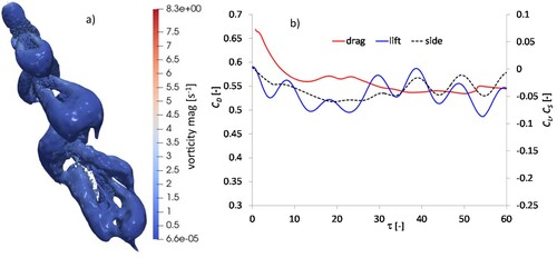
As mentioned in section 3.1.1, for the case of Re = 300, we estimate N_r,k and predict the corresponding computational time of parallelization of the MAST algorithm assuming different N_p number of processors. The maximum N_r,k is 3847. Neglecting the time ϵ and the other parallelization costs, the MAST solution time T_MAST would be equal to (86) $T_{MAST}=\sum _{i=1,N_{iter}}\left(\sum _{r=1,N_{R,k}}\left(Int\left(\frac{N_{r,k}}{N_p}\right)+1\right)\right)2T_T$(86) where N_iter is the number of time steps and N_R,k is the number of ranks at iteration k. This time is of course larger than the time T_min computed assuming all available processors working together, because N_r,i can be smaller than N_p and the ratio between T_MAST and T_min grows along with N_p.

See in Table 6 the ratios T_MAST / T_T and T_MAST / T_min computed in the simulation of test 3, with a mesh of 2,309,771 tetrahedrons, assuming a number of processors in the range 4-250, at the present time corresponding to small-medium workstations. You can observe that the ratio T_MAST / T_min attains a maximum value of 1.4 with the maximum number of 250 processors. This means that parallelization should work very well with this type of very popular computers even with large size problems.

Table 6. MAST solution time vs. no. of processors.

Np	Tmin/TT	TMAST/TT	TMAST /Tmin
4	676,184,582	680,355,106	1.006
12	225,394,080	229,004,379	1.016
40	67,618,224	71,041,472	1.051
50	54,094,345	57,521,651	1.063
100	27,046,587	30,304,361	1.120
150	18,031,058	20,938,102	1.161
200	13,522,708	16,347,121	1.209
250	10,818,869	15,173,010	1.402

5.3.4. Simulation of blood flow inside aneurism

In this test, we simulated the hemodynamic flow conditions inside a real abdominal aorta affected by a large aneurysm without thrombus in the lumen. The computational domain was computed starting from the kinematic field of a real (44-year-old female) patient-specific aortic wall, obtained from the data recorded by an electrocardiogram-gated computer tomography angiography (CTA) during a stabilized cardiac cycle, as described in (Aricò et al., 2020 and cited references).

Besides the CTA images, additional input data were the measurements, in a resting condition, of pressure (on the left arm) and aorta volumetric flow rate (in the carotid artery), during a stabilized cardiac cycle (Aricò et al., 2020). The cardiac cycle T_c of the patient was 0.83333 s.

The real aortic segment was approximately 0.16 m long (see Figure 20(a)). The computational domain was extended with respect to the real one by means of two transition stretches, and the real cross-sections were linearly morphed into circles of equivalent radii $r=\sqrt{A/\pi }$ (Figure 20(a)). The diameters of the inflow and outflow artificial sections, D_i and D_o, are 0.03213 and 0.0256 m, respectively, and the two stretches were approximately D_i long.

Figure 20. (a) Test 4. Real and computational domain. (b) computational mesh. (c) Section of the mesh with a generic plane.

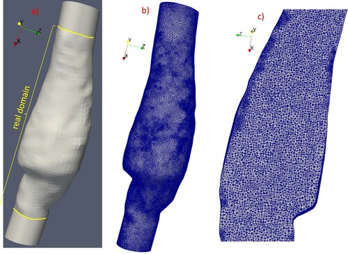
For the numerical model simulations, we set an inflow velocity profile and a uniform spatial pressure distribution along the upstream and downstream sections of the computational domain, respectively. The BCs of the present model were obtained as described in Aricò et al. (2020) and cited references.

In Figure 21(a) we plot the waveforms of the inflow velocity (obtained by dividing the waveform of the flow rate by the area of the inflow cross-section), and the outlet pressure. The ‘time of the diastolic (systolic) pressure’ is the time corresponding to the minimal (maximal) aortic pressure – tdp (tsp) in Figure 21. tdp and tsp were computed to be 0.0589 and 0.2946 s after the start of the cycle (Nagy et al., 2015).

Figure 21. Test 4. (a) waveforms of mean-in-time inflow velocity and outlet pressure. (b) Womersley inflow velocity profiles at four significant times (from Aricò et al., 2020).

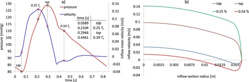
A Womersley velocity profile of the pulsatile flow (Womersley, 1955) was analytically computed for the diameter D_i, as described in Aricò et al. (2020), and assigned to the upstream boundary of the computational domain. The Womersley number α can be regarded as the ratio between the unsteady inertial forces and the viscous forces, and it is defined as (Womersley, 1955) (87) $\alpha =R\sqrt{\frac{\omega }{\nu }}\text{ with }\omega =1/T_c$(87) where R is the radius of the vessel at the boundary section. We set ν = 3.77 × 10⁻⁶ m²/s (blood kinematic viscosity). The original Poiseuille velocity profile is flattened proportionally to the α number. In the present case α is around 24, and Figure 21(b) shows the profiles computed for the significant times listed in the table of Figure 21(a).

The maximum value of the Reynolds number attained during the simulations was approximately 1200, which implies a fully laminar flow.

The computational domain corresponds to the fixed-in-time geometry computed, at the tsp time, applying the procedure proposed in Nagy et al. (2015). The computational mesh had 790,346 tetrahedrons and 146,995 nodes, and the number of cluster is 729,038. The mesh size ranged from 1.e-04 m to 1e-03 m. In Figure 20(b,c) we show the mesh and a zoom of a cutting generic plane. The time step size was 0.01 s and the maximum value of the CFL number computed during the simulations was 3.45.

In Figure 22, for the significant times listed in Figure 21(b), we show the computed velocity and the kinematic pressure fields. The black arrow indicates the main upstream-downstream flow direction. At tdp, the pressure gradient is oriented according to the main upstream-downstream direction. The velocity profile in the upstream portion of the studied reach is almost uniform along the radial vessel direction, and, close to the walls, recirculating flow zones arise (see the zoom in Figure 23). These recirculating flows could be generated by the inflow velocity computed in the most lateral part of the Womersley profile (see Figure 21(b)). The blood flow decelerates in the central region of the aorta, due to the enlargement of the vessel because of the aneurysm, and accelerates downstream of the aneurysm, due to the reduction of the section of the vessel. Due to the reduction of the inflow velocity assigned at the inflow section, from time 0.25 T_c to tsp, and the corresponding increase of the assigned outlet pressure in the same time interval (see Figure 21), the pressure gradient along the principal flow direction changes sign, becoming downstream-upstream oriented. The recirculating flow velocity zones close to the lateral walls then disappear, since the boundary Womersley velocities assigned at the inflow section are inward oriented. At time 0.54 T_c, the flow recirculation close to the vessel walls is stronger than at tdp. The size of the portion of the inflow section where the leaving Womersley velocities are set is similar to the one where the incoming velocities are assigned, and their norm is comparable to (or greater than) the values of the inflow velocity norm (see Figure 21(b)). Vorticities also arise in the central and downstream portions of the aortic vessel, as shown in the zoom of the velocity vector (Figure 22).

Figure 22. Test 4. Computed velocity vectors and kinematic pressure at the significant times in Figure 21.

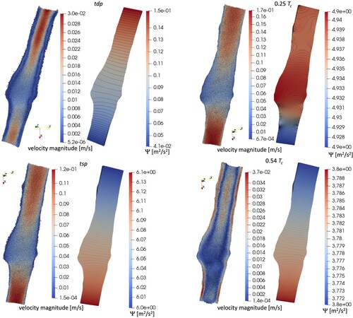
Figure 23. Test 4. Zoom of the velocity fields for tdp and 0.54 T_c.

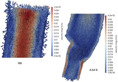
In Figure 24 we plot the values of the velocity components computed along the axis of the aneurism, shown in Figure 25, at four different times. The origin of the coordinates along the axis is also shown in Figure 25. These results are marked as ‘u (v, w) m1’. In Figure 24, we also superimpose the results obtained using a refined mesh, with 3,361,925 tetrahedrons, 599,988 nodes, and 3,116,998 clusters, marked as ‘u (v, w) m2’. The scatters between the two solutions are almost negligible.

Figure 24. Test 4. Velocity components computed along the axis shown in Figure 25, for two meshes.

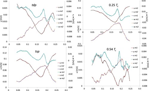
Figure 25. Test 4. Initial and final axis position.

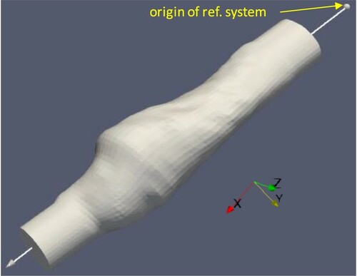
6. Conclusions

A new algorithm for the numerical solution of the 3D Navier–Stokes equations for incompressible fluids has been presented and validated with synthetic tests. The algorithm is radically new and is based on the Raviart-Thomas first order spatial discretization of pressure and velocity. The convective terms were solved using the Marching in Space and Time (MAST) technique, previously applied only to groundwater transport and shallow water problems. The algorithm has the following merits with respect to the many other competitors: (1) It can be applied to any tetrahedral, unstructured and non-Delaunay mesh, generated inside irregular boundaries; (2) it fully preserves mass conservation, (3) the time step size is not constrained by the CFL limit, (4) the CPU time required for the solution of a single time step, with a single physical processor, grows with a β power almost equal to 1.1, due to the solution of linear systems with matrices that are always positive-definite, holding the M-property, factorized only once at the beginning of the first time step.

Code parallelization and introduction of a turbulence model to solve the turbulence structures within the element scale would make MAST-RT0 model ready to solve also many other problems of great interest, like Fluid-Structure Interactions (FSI), flows around moving boundaries (e.g. swimming fishes) (e.g. Salih et al., 2019), sloshing tanks (e.g. Ghalandari et al., 2019) and many others.

Disclosure statement

No potential conflict of interest was reported by the author(s).

Notes

1 www.hsl.rl.ac.uk/catalogue/kb07.html, 1962.

2 hsl.rl.ac.uk/catalogue/mi21.html, 2013.

3 www.qhull.org/html/index.htm, 2020, and cited references.

4 www.paraview.org, 2020.

Appendix 1. The Order subroutine

Call ET (j,k) the index of the jth tetrahedron neighbor to tetrahedron k and Fl (j,k) the flux between tetrahedrons k and ET (j,k). ET (j,k) = 0 if the jth face of tetrahedron k is a boundary face. Flux FL (j,k) is positive if it goes from k to ET (j,k), negative otherwise. We assume the fluxes of two neighbor tetrahedrons k and kp to have the same norm and opposite sign in the shared face. The Order input are the integer matrices ET, FL and the initial IORD vector.

Call INV(k) the position m of tetrahedron k in the IORD vector, such that INV(IORD(m)) = m. Vector INV is initialized according to the input IORD vector. Initialize also two other auxiliary vectors AUX and BACK and one auxiliary matrix JC with size[4, N_T], where N_T is the number of tetrahedrons. All vectors RANK, BACK and JC are initialized with 0.

The Order algorithm computes the vector RANK and updates the vector IORD. The output vector IORD provides, for each index m, the tetrahedron k = IORD(m) with the following properties: (A1) $\begin{array}{rl}(\text{RANK}(\text{ET}(j,k))& >0\text{ or }\text{JC }(j,k)\ne 0)\text{ if }(\text{FL }(j,k)\\ & <0\text{ and }\text{ET }(j,k)>0)j=1,\dots ,4\end{array}$(A1) (A2) $\begin{array}{rl}(\text{RANK}(k)& >\text{RANK }(\text{ET}(j,k))\text{ or }\text{JC }(j,k)\ne 0)\\ & \text{if }(\text{FL }(j,k)<0\text{ and }\text{ET }(j,k)>0)\\ & j=1,\dots ,4\end{array}$(A2) (A3) $\begin{array}{rl}(\text{INV}(\text{ET}(j,k))& <\text{INV }(k)\text{ or }\text{JC }(j,k)\ne 0)\\ & \text{ if }(\text{FL }(j,k)<0\text{ and }\text{ET}(j,k)>0)\\ & \text{for any value }k\\ & =\text{iord }(s)\text{ and }0<s<m\end{array}$(A3)

The general strategy is to compute the mth tetrahedron of IORD and its rank RANK(IORD(m)) after the computation of the previous tetrahedrons IORD(1), … , IORD (m–1) and their rank. Order adopts the following subroutines, where apex i marks input variables and apex o marks output variables:

A1.1. Subroutine Switch

Input: nx, AUX, IORD, INV, FL, ET, RANK

Output: RANK, IORD, INV

Given the known index r = AUX(nx) of a tetrahedron which satisfies constraints A1 and has RANKⁱ(r) = 0, compute the new rank of r as the maximum rank of the neighbor tetrahedrons that satisfy constraint (A1), plus one. This allows tetrahedron r to satisfy also requirement A2. Switch the position of tetrahedrons r and IORDⁱ(m) in the IORD^o vector, by setting: s = INVⁱ(r), IORD^o(m) = r, IORD^o(s) = IORDⁱ(,m), INV^o(r) =m, INV^o(IORDⁱ(m)) = s. See the flow-chart in Figure A1.

A1.2. Subroutine Search

Input: nx, AUX, IORD, INV, FL, ET, RANK, BACK, JC

Output: nx, AUX, BACK, RANK, IORD, INV, JC

Call BACK(k) the neighbor of tetrahedron k with RANK(k) = 0 and RANK(BACK(k)) = 0 with the maximum flux going from to BACK(k) to k. Given a length nxⁱ≥ 1, check if constraint (A1) is satisfied for k = AUX(nx). If it is satisfied, apply Switch and set nx^o = nxⁱ – 1. Otherwise, select the neighbor tetrahedron kp with the minimum (maximum absolute value) entering flux smaller than zero and with RANKⁱ(kp) = 0. If BACK(kp) ≠ 0, we have a loop. In this case apply subroutine Cut and iterate the check. If constraint (A1) is not satisfied, select the neighbor tetrahedron kp with RANK(kp) = 0 and minimum entering flux, set BACK(k) = kp, update nx^o with nxⁱ + 1, set AUX(nx^o) = kp, and iterate until constraint (A1) is satisfied. See the flow-chart in Figure A2.

A1.3. Subroutine Cut

Input: nx, AUX, BACK, JC, FL, ET

Output: nx, BACK, JC

If a loop is found, compute the index mb and the tetrahedron kb = AUXⁱ (mb) corresponding to the minimum positive flux going from BACK (AUXⁱ (m)) to AUXⁱ (m) for mp ≤ m ≤ nxⁱ, where AUXⁱ (mp) = BACK (AUXⁱ (nxⁱ)). Set nx^o = mb and BACK^o (AUXⁱ (m)) = 0, for mb ≤ m ≤ nxⁱ. Set ka = BACK0ⁱ (kb), JC^o (n1,ka) = kb and JC^o (n2,kb) = ka, where n1 and n2 are the local indices of the face common to tetrahedrons ka and kb. See the flow-chart in Figure A3.

In Order we loop the index p from 1 to nel. At each iteration, if nx > 0 we apply Search. If nx = 0, we test the tetrahedron k = IORD(p). If constraint (A1) is satisfied, we apply Switch. If it is not satisfied, we set nx = 1, AUX(nx) = k and apply Search. See the flow-chart in Figure A4.

Observe that, if zero loops and zero flux sign changes occur, the solution obtained in the MAST procedure is the same with any adopted sorting rule providing a sequence vector IORD also different from the vector computed in the Order subroutine, if constraint (A3) is satisfied for all the tetrahedrons. Due to loop cuts and flux sign changes, this is not true and a much better solution turns out to be the one obtained by solving sequentially all the tetrahedrons with the same rank, starting from 1, also using parallel computing if available. Any open source subroutine, like QUICKSORT, can be used to order all the tetrahedrons according to their rank value after the RANK solution of Order is found.

See the flow-chart of the Order, Search, Cut and Switch subroutines in Figures A1–A4.

Figure A1. Flow-chart of the Order subroutine.

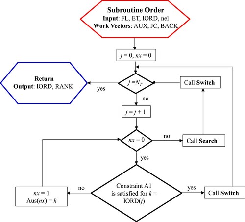
Figure A2. Flow-chart of the Search subroutine.

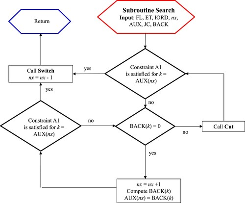
Figure A3. Flow-chart of the Cut subroutine.

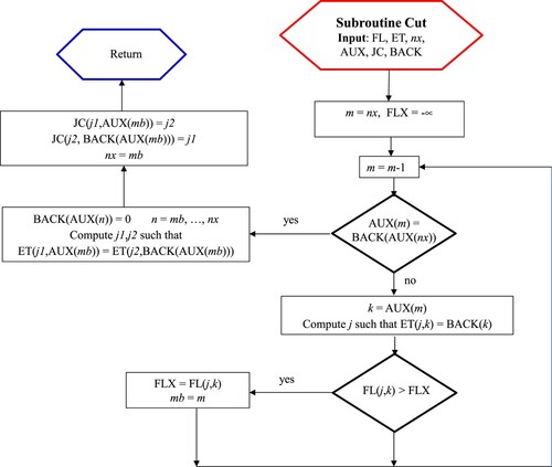
Figure A4. Flow-chart of the Switch subroutine.

References

- Aguerre, H. J., Venier, C. M., Pairetti, C. I., Márquez Damián, S., & Nigro, N. M. (2020). A SIMPLE-based algorithm with enhanced velocity corrections: The COMPLEX method. Computers & Fluids, 198(15), Article 104396. https://doi.org/https://doi.org/10.1016/j.compfluid.2019.104396
- Aricò, C., Nasello, C., & Tucciarelli, T. (2007). A marching in space and time (MAST) solver of the shallow water equations. Part II: The 2D model. Advances in Water Resources, 30(5), 1253–1271. https://doi.org/https://doi.org/10.1016/j.advwatres.2006.11.004
- Aricò, C., Sinagra, M., Begnudelli, L., & Tucciarelli, T. (2011). MAST-2D diffusive model for flood prediction on domains with triangular Delaunay unstructured meshes. Advances in Water Resources, 34(11), 1427–1449. https://doi.org/https://doi.org/10.1016/j.advwatres.2011.08.002
- Aricò, C., Sinagra, M., Nagy, R., Napoli, E., & Tucciarelli, T. (2020). Investigation of the hemodynamic flow conditions and blood-induced stresses inside an abdominal aortic aneurysm by means of a SPH numerical model. International Journal for Numerical Methods in Biomedical Engineering, 36, 3263. https://doi.org/https://doi.org/10.1002/cnm.3263
- Aricò, C., Sinagra, M., & Tucciarelli, T. (2012). The MAST-edge centred lumped scheme for the flow simulation in variably saturated heterogeneous porous media. Journal of Computational Physics, 231(4), 1387–1425. https://doi.org/https://doi.org/10.1016/j.jcp.2011.10.012
- Aricò, C., Sinagra, M., & Tucciarelli, T. (2013a). Monotonic solution of flow and transport problems in heterogeneous media using Delaunay unstructured triangular meshes. Advances in Water Resources, 52(4), 132–150. https://doi.org/https://doi.org/10.1016/j.advwatres.2012.09.006
- Aricò, C., Sinagra, M., & Tucciarelli, T. (2013b). Anisotropic potential of velocity fields in real fluids: Application to the MAST solution of shallow water equations. Advances in Water Resources, 62, 13–36. https://doi.org/https://doi.org/10.1016/j.advwatres.2013.09.010
- Aricò, C., & Tucciarelli, T. (2007a). MAST solution of advection problems in irrotational flow fields. Advances in Water Resources, 30(3), 665–685. https://doi.org/https://doi.org/10.1016/j.advwatres.2006.03.007
- Aricò, C., & Tucciarelli, T. (2007b). A marching in space and time (MAST) solver of the shallow water equations. Part I: The 1D model. Advances in Water Resources, 30(5), 1236–1252. https://doi.org/https://doi.org/10.1016/j.advwatres.2006.11.003
- Aricò, C., & Tucciarelli, T. (2009). The MAST-FV/FE scheme for the simulation of thermohaline processes in variable density saturated porous media. Journal of Computational Physics, 228(4), 1234–1274. https://doi.org/https://doi.org/10.1016/j.jcp.2008.10.015
- Aricò, C., & Tucciarelli, T. (2013). Monotonic solution of heterogeneous anisotropic diffusion problems. Journal of Computational Physics, 252, 219–249. https://doi.org/https://doi.org/10.1016/j.jcp.2013.06.017
- Auricchio, F., Beirão da Veiga, L., Brezzi, F., & Lovadina, C. (2017). Mixed finite element methods. In Encyclopedia of computational mechanics. 2nd ed. (pp. 1–53). https://doi.org/https://doi.org/10.1002/9781119176817.ecm2004
- Bassi, F., & Rebay, S. (1997). A high-order accurate discontinuous finite element method for the numerical solution of the compressible Navier-Stokes equations. Journal of Computational Physics, 131, 267–279. https://doi.org/https://doi.org/10.1006/jcph.1996.5572
- Bazilevs, Y., Takizawa, K., & Tezduyar, T. E. (2013). Computational fluid-structure interaction: Methods and applications. Wiley. https://doi.org/https://doi.org/10.1002/9781118483565
- Beirão da Veiga, L., Lovadina, C., & Vacca, G. (2018). Virtual elements for the Navier-Stokes problems on polygonal meshes. SIAM Journal on Numerical Analysis, 56(3), 1210–1242. https://doi.org/https://doi.org/10.1137/17M1132811
- Boppana, V. B. L., & Gajjar, J. S. B. (2010). Global flow instability in a lid-driven cavity. International Journal for Numerical Methods in Fluids, 62, 827–853. https://doi.org/https://doi.org/10.1002/fld.2040
- Botella, O., & Peyret, R. (1998). Benchmark spectral results on the lid driven cavity flow. Computers & Fluids, 27, 421–433. https://doi.org/https://doi.org/10.1016/S0045-7930(98)00002-4
- Braaten, M. E., & Shyy, W. (1986). Comparison of iterative and direct method for viscous flow, calculations in body-fitted coordinates. International Journal for Numerical Methods in Fluids, 6, 325–349. https://doi.org/https://doi.org/10.1002/fld.1650060603
- Brankin, R. W., Gladwell, I., & Shampine, L. F. (1993). RKSUITE: A suite of explicit Runge-Kutta codes. Computer Science. https://doi.org/https://doi.org/10.1142/9789812798886_0004
- Busto, F., Ferrìn, J. L., Toro, E. F., & Vazquez-Cendon, M. E. (2018). A projection hybrid high order finite volume/finite element method for incompressible turbulent flows. Journal of Computational Physics, 353, 169–192. https://doi.org/https://doi.org/10.1016/j.jcp.2017.10.004
- Calhoun, D. (2002). A Cartesian grid method for solving the two-dimensional stream function-vorticity equations in irregular regions. Journal of Computational Physics, 176, 231–275. https://doi.org/https://doi.org/10.1006/jcph.2001.6970
- Chorin, A. J. (1968). Numerical solution of the Navier-Stokes equations. Mathematics of Computation, 22, 745–762. https://doi.org/https://doi.org/10.2307/2004575
- Dalal, A., Eswaran, V., & Biswas, G. (2008). A finite-volume method for Navier-Stokes equations on unstructured meshes. Numerical Heat Transfer, Part B: Fundamentals, 54(3), 238–259. https://doi.org/https://doi.org/10.1080/10407790802182653
- Darwish, M., Abdel Aziz, A., & Moukalled, F. (2015). A coupled pressure-based finite-volume solver for incompressible two-phase flow. Numerical Heat Transfer, Part B: Fundamentals, 67, 47–74. https://doi.org/https://doi.org/10.1080/10407790.2014.949500
- Darwish, M., Sraj, I., & Moukalled, F. (2009). A coupled finite volume solver for the solution of incompressible flows on unstructured grids. Journal of Computational Physics, 228, 180–201. https://doi.org/https://doi.org/10.1016/j.jcp.2008.08.027
- Forsyth, P. A. (1991). A control volume finite element approach to NAPL groundwater contamination. SIAM Journal on Scientific and Statistical Computing, 12, 1029–1057. https://doi.org/https://doi.org/10.1137/0912055
- Fortin, M. (1981). Old and new finite elements for incompressible flows. International Journal for Numerical Methods in Fluids, 1, 347–364. https://doi.org/https://doi.org/10.1002/fld.1650010406
- Gao, W., Liu, R. X., & Li, H. (2012). A hybrid vertex-centered finite volume/element method for viscous incompressible flows on non-staggered unstructured meshes. Acta Mechanica Sinica, 28(2), 324–334. doi:https://doi.org/10.1007/s10409-012-0038-2
- Ghalandari, M., Bornassi, S., Shamshirband, S., Mosavi, A., & Chau, K. W. (2019). Investigation of submerged structures’ flexibility on sloshing frequency using a boundary element method and finite element analysis. Engineering Applications of Computational Fluid Mechanics, 13(1), 519–528. https://doi.org/https://doi.org/10.1080/19942060.2019.1619197
- Ghia, U., Ghia, K. N., & Shin, C. T. (1982). High-resolutions for incompressible flow using the Navier-Stokes equations and a multigrid method. Journal of Computational Physics, 48, 387–411. https://doi.org/https://doi.org/10.1016/0021-9991(82)90058-4
- Gingold, R. A., & Monaghan, J. J. (1977). Smoothed particle hydrodynamics-theory and application to non-spherical stars. Monthly Notices of the Royal Astronomical Society, 181, 375–389. https://doi.org/https://doi.org/10.1093/mnras/181.3.375
- Gosman, A. D., Koosinlin, M. L., Lockwad, F. C., & Spalding, D. B. (1976). Transfer of heat in rotating systems. ASME M. 76-GT 25. https://doi.org/https://doi.org/10.1115/76-GT-25
- Guermond, J. L., Minev, P., & Shen, J. (2006). An overview of projection methods for incompressible flows. Computer Methods in Applied Mechanics and Engineering, 195, 6011–6045. https://doi.org/https://doi.org/10.1016/j.cma.2005.10.010
- Hanby, R. F., & Silvester, D. J. (1996). A comparison of coupled and segregated iterative solution techniques for incompressible swirling flow. International Journal for Numerical Methods in Fluids, 22, 353–373. https://doi.org/https://doi.org/10.1002/(SICI)1097-0363(19960315)22:5<353::AID-FLD327>3.0.CO;2-Z
- Hang, S. (2015). Tetgen, a Delaunay-based quality tetrahedral mesh generator. ACM Transactions on Mathematical Software, 41(2), 1. https://doi.org/https://doi.org/10.1145/2629697
- Harlow, F. H., & Welch, J. E. (1965). Numerical calculation of three-dimensional time dependent viscous incompressible flow of fluid with free surface. Physics of Fluids, 8(12), 2182–2189. https://doi.org/https://doi.org/10.1063/1.1761178
- Hughes, T. J. R., Liu, W. K., & Brooks, A. (1979). Finite element analysis of incompressible viscous flows by the penalty function formulation. Journal of Computational Physics, 30(1), 1–60. https://doi.org/https://doi.org/10.1016/0021-9991(79)90086-X
- Hunt, J. C. R., Wray, A., & Moin, P. (1988). Eddies, stream, and convergence zones in turbulent flows. Center for Turbulence Research, Report CTR-S88.
- Joe, B. (1986). Delaunay triangular meshes in convex polygons. SIAM Journal on Scientific and Statistical Computing, 7, 514–539. https://doi.org/https://doi.org/10.1137/0907035
- Johnson, T. A., & Patel, V. C. (1999). Flow past a sphere up to a Reynolds number of 300. Journal of Fluid Mechanics, 378, 19–70. https://doi.org/https://doi.org/10.1017/S0022112098003206
- Kim, D., & Choi, H. (2000). A second-order time-accurate finite volume method for unsteady incompressible flow on hybrid unstructured grids. Journal of Computational Physics, 162, 411–428. https://doi.org/https://doi.org/10.1006/jcph.2000.6546
- Kim, J., & Moin, P. (1985). Application of a fractional-step method to incompressible Navier-Stokes equations. Journal of Computational Physics, 59, 308–323. https://doi.org/https://doi.org/10.1016/0021-9991(85)90148-2
- Kuhlmann, H. C., & Romanò, F. (2019). The lid-driven cavity. In Computational methods in applied sciences, Vol. 50 (pp. 233–309). https://doi.org/https://doi.org/10.1007/978-3-319-91494-7_8
- Lehrenfeld, C., & Schöberl, J. (2016). High order exactly divergence-free hybrid discontinuous Galerkin methods for unsteady incompressible flows. Computer Methods in Applied Mechanics and Engineering, 307, 339–361. https://doi.org/https://doi.org/10.1016/j.cma.2016.04.025
- Letniowski, F. W. (1992). Three-dimensional Delaunay triangulations for finite element approximations to a second-order diffusion operator. SIAM Journal on Scientific and Statistical Computing, 13, 765–770. https://doi.org/https://doi.org/10.1137/0913045
- Li, X. Y., & Teng, S. H. (2001, January 7–9). Generating well-shaped Delaunay meshes in 3D. Proceedings of the Twelfth Annual Symposium on Discrete Algorithms, Washington, DC, USA. Association for Computing Machinery. https://doi.org/https://doi.org/10.1145/365411.365416
- Liu, X., & Chen, Z. (2019). The nonconforming virtual element method for the Navier-Stokes equations. Advances in Computational Mathematics, 45, 51–74. https://doi.org/https://doi.org/10.1007/s10444-018-9602-z
- Lucy, L. B. (1977). A numerical approach to the testing of the fission hypothesis. The Astronomical Journal, 82(12), 1013–1024. https://doi.org/https://doi.org/10.1086/112164
- Malan, A. G., Lewis, R. W., & Nithiarasu, P. (2002). An improved unsteady, unstructured, artificial compressibility, finite volume scheme for viscous incompressible flows: Part I. Theory and implementation. International Journal for Numerical Methods in Engineering, 54, 695–714. https://doi.org/https://doi.org/10.1002/nme.447
- Mathur, S. R., & Murthy, J. Y. (1997). A pressure-based method for unstructured meshes. Numerical Heat Transfer, Part B: Fundamentals, 31(2), 195–215. https://doi.org/https://doi.org/10.1080/10407799708915105
- Mazhar, Z. (2016). A novel fully implicit block coupled solution strategy for the ultimate treatment of the velocity–pressure coupling problem in incompressible fluid flow. Numerical Heat Transfer, Part B: Fundamentals, 69(2), 130–149. https://doi.org/https://doi.org/10.1080/10407790.2015.1093787
- Nagy, R., Csobay-Novák, C., Lovas, A., Sótonyi, P., & Bojtár, I. (2015). Non-invasive in vivo time-dependent strain measurement method in human abdominal aortic aneurysms: Towards a novel approach to rupture risk estimation. Journal of Biomechanics, 48(10), 1876–1886. https://doi.org/https://doi.org/10.1016/j.jbiomech.2015.04.030
- Oger, G., Doring, M., Alessandrini, B., & Ferrant, P. (2007). An improved SPH method: Towards higher order convergence. Journal of Computational Physics, 225(2), 1472–1492. https://doi.org/https://doi.org/10.1016/j.jcp.2007.01.039
- Ozoe, H., & Tao, W. Q. (2001). A modified pressure-correction scheme for the SIMPLER method, MSIMPLER. Numerical Heat Transfer, Part B: Fundamentals, 39(5), 435–449. https://doi.org/https://doi.org/10.1080/104077901750188831
- Pai, S. A., Prakash, P., & Patnaik, B. S. V. (2013). Numerical simulation of chaotic mixing in lid drive cavity: Effect of passive plug. Engineering Applications of Computational Fluid Mechanics, 7(3), 406–418. https://doi.org/https://doi.org/10.1080/19942060.2013.11015481
- Patankar, S. V. (1980). Numerical heat transfer and fluid flow. https://doi.org/https://doi.org/10.1201/9781482234213
- Patankar, S. V. (1981). A calculation procedure for two-dimensional elliptic situations. Numerical Heat Transfer, 4(4), 409–425. https://doi.org/https://doi.org/10.1080/01495728108961801
- Perot, J. B. (2000). Conservation properties of unstructured staggered mesh schemes. Journal of Computational Physics, 159, 58–89. https://doi.org/https://doi.org/10.1006/jcph.2000.6424
- Perron, S., Boivin, S., & Herard, V. (2004). A finite volume method to solve the 3D Navier-Stokes equations on unstructured collocated meshes. Computers & Fluids, 33, 1305–1333. https://doi.org/https://doi.org/10.1016/j.compfluid.2003.10.006
- Plana Fattori, A., Chantoiseau, E., Doursat, C., & Flick, D. (2013). Two-way coupling of fluid-flow, heat transfer and product transformation during heat treatment of starch suspension inside tubular exchanger. Engineering Applications of Computational Fluid Mechanics, 7(3), 334–345. https://doi.org/https://doi.org/10.1080/19942060.2013.11015475
- Ploumhans, P., Winckelmans, G. S., Salmon, J. K., Leonard, A., & Warren, M. S. (2002). Vortex methods for direct numerical simulation of three-dimensional bluff body flows: Application to the sphere at Re = 300, 500, and 1000. Journal of Computational Physics, 178, 427–463. https://doi.org/https://doi.org/10.1006/jcph.2002.7035
- Raviart, P. A., & Thomas, J. M. (1977). A mixed finite element method for 2-nd order elliptic problems. In I. Galligani & E. Magenes (Eds.), Mathematical aspects of finite element methods. Lecture Notes in Mathematics, Vol. 606. Springer. https://doi.org/https://doi.org/10.1007/BFb0064470
- Roos, F. W., & Willmarth, W. W. (1971). Some experimental results on sphere and disk drag. AIAA Journal, 9, 285–291. https://doi.org/https://doi.org/10.2514/3.6164
- Sakamoto, H., & Haniu, H. (1990). A study of vortex shedding from spheres in a uniform flow. Journal of Fluids Engineering, 112, 386. https://doi.org/https://doi.org/10.1115/1.2909415
- Salih, S. Q., Aldlemy, M. S., Rasani, M. R., Ariffin, A. K., Ya, T. M. Y. S. T., Al-Ansari, N., Yaseen, Z. M. M., & Chau, K. W. (2019). Thin and sharp edges bodies-fluid interaction simulation using cut-cell immersed boundary method. Engineering Applications of Computational Fluid Mechanics, 13(1), 860–877. https://doi.org/https://doi.org/10.1080/19942060.2019.1652209
- Schöberl, J. (1997). NETGEN – an advancing front 2D/3D-mesh generator based on abstract rules. Computing and Visualization in Science, 1(1), 41–52. https://doi.org/https://doi.org/10.1007/s007910050004
- Shyy, W., & Mittal, R. (1998). Solution methods for the incompressible Navier-Stokes equations. In R. W. Johnson (Ed.), Handbook of fluid dynamics (pp. 31.1–31.33). CRC Press. ISBN 9780849325090.
- Sungsu, L. (2000). A numerical study of the unsteady wake behind a sphere in a uniform flow at moderate Reynolds numbers. Computers & Fluids, 29, 639–667. https://doi.org/https://doi.org/10.1016/S0045-7930(99)00023-7
- Tao, W. Q. (2001). Numerical heat transfer (2nd ed.). Xi'an Jiaotong University Press. ISBN 10: 7560514367/ISBN 13: 9787560514369.
- Taylor, G. I., & Green, A. E. (1937). Mechanism of the production of small eddies from large ones. Proceedings of the Royal Society of London. Series A – Mathematical and Physical Sciences, 158, 499–521. https://doi.org/https://doi.org/10.1098/rspa.1937.0036
- Tomboulides, A. G. (1993). Direct and Large-Eddy simulation of wake flows: Flow past a sphere, PhD thesis, Princeton University.
- Toro, E. F., Müller, L. O., & Siviglia, A. (2020). Bounds for wave speeds in the Riemann problem: Direct theoretical estimates. Computers & Fluids, 209. https://doi.org/https://doi.org/10.1016/j.compfluid.2020.104640
- Toro, E. F., & Vazquez-Cendon, M. E. (2012). Flux splitting schemes for the Euler equations. Computers & Fluids, 70, 1–12. https://doi.org/https://doi.org/10.1016/j.compfluid.2012.08.023
- Vidovic, D., Segal, A., & Wesseling, P. (2004). A superlinearly convergent finite volume method for the incompressible Navier-Stokes equations on staggered unstructured grids. Journal of Computational Physics, 198, 159–177. https://doi.org/https://doi.org/10.1016/j.jcp.2004.01.005
- Vrahliotis, S., Pappou, T., & Tsangaris, S. (2012). Artificial compressibility 3-D Navier-Stokes solver for unsteady incompressible flows with hybrid grids. Engineering Applications of Computational Fluid Mechanics, 6(2), 248–270. https://doi.org/https://doi.org/10.1080/19942060.2012.11015419
- Womersley, J. R. (1955). Method for the calculation of velocity, rate of flow and viscous drag in arteries when the pressure gradient is known. The Journal of Physiology, 127(3), 553–563. https://doi.org/https://doi.org/10.1113/jphysiol.1955.sp005276
- Xue, S. C., & Burton, G. W. (2013). A finite volume formulation for transient convection and diffusion equations with unstructured distorted grids and its applications in fluid flow simulations with a collocated variable arrangement. Computer Methods in Applied Mechanics and Engineering, 253, 146–159. https://doi.org/https://doi.org/10.1016/j.cma.2012.09.016
- Younes, A., Ackerer, P., & Chavent, G. (2004). From mixed finite elements to finite volumes for elliptic PDEs in two and three dimensions. International Journal for Numerical Methods in Engineering, 59, 365–388. https://doi.org/https://doi.org/10.1002/nme.874
- Younes, A., Ackerer, P., & Lehmann, F. (2006). A new mass lumping scheme for the mixed hybrid finite element method. International Journal for Numerical Methods in Engineering, 67(1), 89–107. https://doi.org/https://doi.org/10.1002/nme.1628
- Zienkiewicz, O., Taylor, R., & Nithiarasu, P. (2013). The finite element method for fluid dynamics. Elsevier. https://doi.org/https://doi.org/10.1016/C2009-0-26328-8