Influence of blade inlet angle on the performance of a single blade centrifugal pump

Abstract

Single blade centrifugal pump is suitable for transporting sewage water with large obstacles in diameter, which is required to achieve high performance. The blade inlet angle is a parameter that affects the performance of the single blade centrifugal pump. However, the selection of blade inlet angle is frequently based on experiences and demonstrates certain arbitrariness. Therefore, six impellers with different blade inlet angles are designed using ANSYS Bladegen and NX software. These impellers are categorized into Groups 1 and 2. The blade inlet angle of the impellers in Group1/Group2 increases/decreases from the front shroud to the rear one, respectively. Subsequently, the numerical simulation is carried out to investigate the effect of the blade inlet angle on the performance of the single blade pump. The blade inlet angle has more obvious influence on the head, efficiency, and shaft power for the impellers in Group 1 than those in Group 2. The lowest pressure is negative for one of the impellers in Group 1. Moreover, an optimum blade inlet angle improves the pump performance. In addition, the alternating load is small on the blades of the impellers in Group 2. The present results are helpful in designing the single blade centrifugal pump and improving its performance.

KEYWORDS:

• Single blade centrifugal pump
• blade inlet angle
• numerical calculation
• external characteristics

1. Introduction

Environmental protection has been paid increasing attention with the sustained and rapid economic development, together with the continuous advancement of urbanization. Building and improving various types of sewage treatment facilities is necessary. Thus, the research on sewage pumps becomes very urgent. For example, the single blade centrifugal pump is investigated as a good case. This type of pump is a special category of centrifugal pumps. It has a single flow channel that is formed by a large wrap angle envelope (Tan et al., 2017). Given that the single blade pump only has one blade, it provides a large channel cross section for the fluid flow (Michael et al., 2009). Thus, this type of pump is commonly used as the sewage pump to transport substances that contain solids to avoid clogging disturbance. However, the structure with low blade number faces great challenges, such as low efficiency, pressure fluctuation, and hydrodynamic unbalance (Aoki, 1984; Pei, Yuan, & Dohmen, 2012b).

To improve the sewage pump performance, many researchers have performed studies using theoretical, experimental, and numerical methods. Nishi et al. (2006) and Nishi et al. (2009) applied the CFD analysis to predict the performance of single blade sewage pump to reduce radial force fluctuation components and proposed a method for designing the impeller of single blade centrifugal pumps. Benra et al. (2005) investigated the effect of the impeller position on flow parameters through numerical and experimental methods. Moreover, De Souza et al. (2008) and De Souza et al. (2010) optimized the single blade impeller through design of experiments and computational fluid dynamics (CFD), proposed a novel volute design method with the constant speed method, and applied the proposed method to a single blade impeller. Benra and Dohmen (2008) investigated the radial force of a single blade pump through experiments and CFD software. Subsequently, they employed numerical and PIV schemes to verify the reliability of a Navier–Stokes solver that predicts the transient flow in a single blade pump. Pei, Dohmen & Yuan (2012a) studied the vibration and periodic unstable flow that originated from the single blade pump under non-design conditions by using numerical and experimental methods. Pei et al. (2013) investigated the periodic unsteadiness in the rotor and volute domains for the normal operation quantitatively. Tan et al. (2018) obtained the characteristics of the fluid force that induced the vibration of a single blade pump under different operating conditions. Wang, Long & Yang (2020) and Wang, Long & Wang (2020) studied the influence of impeller blade structure on pump performance.

The aforementioned review indicates that most of the studies are focused on design methods and analyzing the unsteady and turbulence flows, and only few research has carried out investigations on the impact of the blade inlet angle on the performance of the single blade centrifugal pump. As a matter of fact, the blade inlet angle affects the degree of blade bending, which further influences the blade area of the inlet flow. Meanwhile, the position of the stagnation point and the appearance of cavitation are affected (Guan, 2011). Therefore, investigating the influence of the blade inlet angle on the pump performance is very necessary.

For the present study, the 3D modeling software is used to determine the blade inlet angle, which has not been conducted before. Six impellers with different blade inlet angles are designed to reveal the impact of the blade inlet angle on the behavior of the single blade centrifugal pump. Then, the CFD simulation is carried out so that the performance of the six impellers is investigated. We hope to obtain some valuable results to evaluate the relationship between the blade inlet angle and the single blade centrifugal pump performance.

2. Computational model

2.1. Studied pump

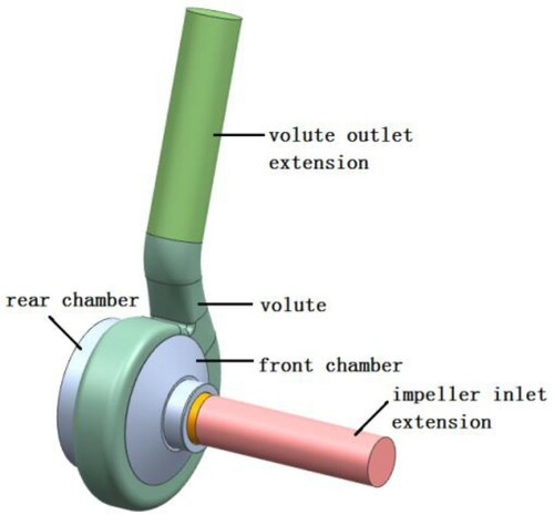
Figure 1 shows the single blade centrifugal pump (the front chamber is removed) investigated in the present study. The volute is stationary, and the impeller rotates at a rotating speed of 2940 rpm. The single blade centrifugal main specifications are listed in Table 1. For the present computation, the water at 25?? is selected as the operating fluid.

Figure 1. View of the single blade centrifugal pump.

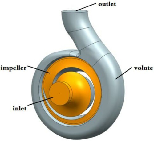
Table 1. Single blade centrifugal pump specifications.

Parameters	Value	Parameters	Value
Head (H)	11 m	Impeller inlet diameter (D1)	45 mm
Rated flow rate (Qd)	20 m^3/h	Impeller outlet diameter (D2)	125 mm
Rotating speed (n)	2940 rpm	Impeller outlet width (b2)	31 mm
Volute inlet diameter (D3)	135 mm	Blade wrap angle (φ)	360°
Volute inlet width (b3)	46 mm	Blade outlet angle (β2)	18°
Specific speed (ns)	132	Blade inlet angle (β1)	To be determined

2.2. Blade inlet angle and impeller model

When the impeller model is established in accordance with the geometric parameters, the profile of the blade leading edge is not a complete surface for the inlet angle higher than 30°. Therefore, the maximum blade inlet angle is set to 30°.

Moreover, Figure 2 shows the axial and plan projection of the single blade impeller. Hence, the three axial streamlines divide the blade axial projection into four equal parts. For the present study, six impellers with different blade inlet angles are designed. The blade inlet angle β₁, which is the inlet angle at the blade suction side, is shown in Figure 2(b). Moreover, the corresponding inlet angles are presented in Table 2, where six impellers are divided into two groups.

Figure 2. Schematic presentation of the impeller. (a) Axial projection (b) Plan projection (removed front shroud).

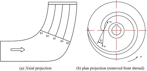
Table 2. Blade inlet angles of six impellers.

Streamline
Impeller	s1	s2	s3	s4	s5	Remarks
Impeller 11	12°	15°	18°	21°	24°
Impeller 12	15°	18°	21°	24°	27°	Group1
Impeller 13	18°	21°	24°	27°	30°
Impeller 21	24°	21°	18°	15°	12°
Impeller 22	27°	24°	21°	18°	15°	Group2
Impeller 23	30°	27°	24°	21°	18°

In Group 1, the streamline inlet angle of each impeller increases 3° from s₁ to s₅, whereas the streamline inlet angle of each impeller in Group 2 decreases 3°. Designed impellers are called impellers 11, 12, 13, 21, 22, and 23. The inlet angles for the same streamlines of impellers 11, 12, and 13 differ sequentially by 3°, whereas those of impellers 21, 22, and 23 are the same. The blade inlet angles at different streamlines for the six impellers are listed in Table 2.

According to design parameters, six impellers with different blade inlet angles and the same other parameters are designed with the Ansys Bladegen and NX software. An isometric view of one of the impellers is shown in Figure 3. The present blade is a twisted one.

Figure 3. Isometric view of a designed single blade impeller. (a) Impeller (b) Blade.

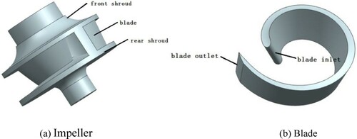
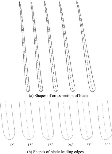
Figure 4(a) shows the evolution of blade cross section for different streamlines. Moreover, the blade thickness gradually increases from streamline s₁ to s₅ regardless of the value of the streamline inlet angle. Figure 4(b) shows the shapes of the blade leading edges for different blade inlet angles. When the inlet angle studied in this paper is relatively small, the pressure side of the blade leading edge is symmetrical to its suction side. However, with the increase in angle, the blade leading edge gradually shows asymmetry.

Figure 4. Blade shapes in different cases. (a) Shapes of cross section of blade, (b) Shapes of blade leading edges.

3. Numerical analyses

Computational fluid dynamics (CFD) is a modern simulation technology that is widely used in various fields (Abadi et al., 2020; Ghalandari et al., 2019; Salih et al., 2019). For the present investigation, CFD software ANSYS CFX is used to simulate the flow in the single blade centrifugal pump. Here, the flow is assumed to be a steady state to simplify the study. Note that CFX is a coupled solver, and governing equations are solved simultaneously.

3.1. Numerical model

Figure 5 indicates that the computational domain includes the impeller inlet extension, front chamber, impeller, rear chamber, volute, and volute outlet extension. Studies (Peng et al., 2020; Zhou et al., 2020) show that extending the impeller inlet and volute outlet in length can improve the stability of inlet and outlet fluid flow, respectively.

Figure 5. Computational domain.

3.2. Grid generation

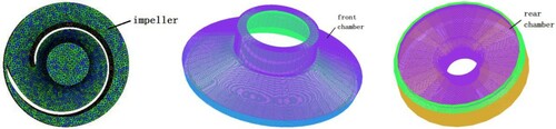
For the present study, the ICEM CFD software is applied to generate the unstructured grids for impeller and volute regions, whereas structured grids are used for other regions. The head and efficiency under the design condition are studied as the criteria to perform the grid independency analysis for impeller 12. Figure 6 shows the calculated results. As the grid number increases, the stability and efficiency of the head also rise. However, when the grid number is more than 2.5×10⁶, both of them vary by less than 0.5%. Thus, based on the results of the grid independency test, the number of grids for all cases is approximately 2.84×10⁶. y⁺ near the walls of the impeller and volute are approximately 80. Figure 7 illustrates the generated grids for the impeller, the front chamber, and the rear chamber.

Figure 6. Grid independency.

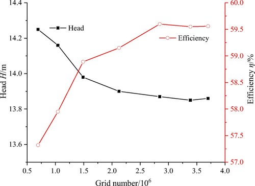
Figure 7. Computational domain and grids of the impeller and chamber.

3.3. Turbulence model

In this steady state case, the Reynolds Average Navier–Stokes equations are used to express the fluid flow in the pump. The turbulence model should be selected to solve the RANS equations. The standard k–ε, RNG k–ε, standard k–ω, and SST k–ω are four commonly used turbulence models. To select a reasonable turbulence model, the calculated results for impeller 12 under the design condition for the four turbulence models are listed in Table 3. As shown in Table 3, the standard k–ε turbulence model can obtain a result similar to the experimental one (the related introduction can be seen in section 5), and the computational time is the shortest among the other models. Hence, in this research, the standard k–ε turbulence model is used to discriminate the turbulence flow. The equations are discretized by finite volume technique. High resolution and first order are adopted for the advection scheme and the turbulence numerics, respectively.

Table 3. Comparison for different turbulence models.

	Head (m)	Efficiency (%)	Relative error in Head (%)	Relative error in Efficiency (%)	Consuming time (minutes)
Experimental results	13.11	57.0
Standard k-ε	13.87	59.6	5.50	4.56	111
RNG k-ε	13.87	58.9	5.50	3.33	209
Standard k-ω	14.04	60.8	7.09	6.67	410
SST k-ω	13.76	59.7	4.96	4.73	217

3.4. Boundary conditions

Scalable wall function is applied to the near wall region. Moreover, the no-slip boundary condition is imposed on the wall surface of the impeller. The wall surface roughness of the volute is defined as 50 µm. The predefined total pressure and the mass flow rate are selected as the inlet and outlet boundary conditions, respectively. The inlet pressure is set to a standard atmospheric pressure, and the inlet turbulence intensity is considered 5%. A region between rotational and stationary ones is connected by a frozen rotor interface, whereas two stationary regions are connected by a general connection interface. To optimize the calculation time and accuracy, the calculation stops when the convergence residual is less than 10⁻⁴.

In addition, models, such as LES, DES and SAS, belong to the scale resolving turbulence model. The characteristics of these models have very high demands for computational resource and cost. Therefore, they are not very suitable for the real engineering question because of a huge computational cost. Limited to the finite computational resource, combining the above analyses, the standard k–ε is chosen here. In addition, although the fluid flow in a single blade centrifugal pump may be unsteady, the present computation shows that some valuable results can be obtained by means of the present condition. Therefore, unsteady computation, unsteady boundary conditions, and the scale resolving turbulence model are not applied here because of complex computations.

4. Results and discussions

4.1. Analyses of the external characteristics

The numerical simulations of the six impellers with different blade inlet angles have been carried out in the foregoing section. The obtained heads of the six impellers are presented in Table 4. The head decreases as the flow rate increases. At each operating point, no fixed meaningful relationship is observed between the head and the blade inlet angle. When the flow rate is 16, 20, and 28 m³/h, impeller 11 in Group 1 has the highest head whereas the head of impeller 13 is the lowest. Furthermore, impeller 22 in Group 2 has the highest head, except for the flow rate of 24m³/h. Table 4 lists the difference between the maximum and the minimum heads of the three impellers in Groups 1 and 2 at each operating point, where the maximum difference is 0.37 m. The influence of the blade inlet angle on the head of Group 1 is more obvious than that of Group 2. Further analyses show that impeller 21 has the lowest head at low flow rates, whereas that of impeller 23 is the smallest at high flow rates. Moreover, the produced head of impeller 21 is the same as that of impeller 23 when the pump works at the design condition. The comparison of the heads between impellers 11 and 21, impellers 12 and 22, and impellers 13 and 23 at different working conditions shows that the maximum head difference is 0.27, 0.32, and 0.18 m, respectively. Furthermore, the produced heads of impellers 11, 22, and 23 are higher for most of working conditions. In other words, when the inlet angle is small, the impeller head in Group 1 is high. Moreover, as the inlet angle increases, the head of the impeller in Group 2 rises.

Table 4. Obtained heads for different impellers.

Q (m^3/h)	12	16	20	24	28
Impeller 11	16.33	15.18	13.92	12.18	10.96
Impeller 12	16.69	15.00	13.87	12.08	10.89
Impeller 13	16.52	14.96	13.55	12.30	10.70
Hmax-Hmin	0.36	0.22	0.37	0.22	0.26
Impeller 21	16.32	14.95	13.73	12.45	10.94
Impeller 22	16.70	15.02	13.75	12.40	10.98
Impeller 23	16.58	14.97	13.73	12.35	10.78
Hmax-Hmin	0.38	0.07	0.02	0.1	0.2

Table 5 shows the efficiency of each impeller. The single blade pump cannot operate at low flow rates because the efficiency abruptly decreases with the flow rate. The influence of the blade inlet angle on the efficiency of Group 1 is more obvious than that of Group 2. When the flow rate is higher than 20 m³/h, the efficiency for the impeller in Group 2 is higher than those of Group 1. The range with a high efficiency of the impeller in Group 2 is wider than that of Group 1. At each operating point, the difference among impeller efficiencies is small. Therefore, the blade inlet angle has a small impact on the efficiency of the single blade centrifugal pump. The comparison of the efficiencies between impellers 11 and 21, impellers 12 and 22, and impellers 13 and 23 indicate that the latter impeller efficiency is higher than that of the former impeller at the design condition, respectively. Moreover, the efficiency impeller 22 is the highest, whereas that of impeller 13 is the lowest. The difference between them is 2.8%. At the design condition, the impellers in Group 2 can improve the pump efficiency well.

Table 5. Obtained efficiencies for different impellers.

Q (m^3/h)	12	16	20	24	28
Impeller 11	50.2	56.0	60.5	61.5	60.1
Impeller 12	49.5	55.0	61.0	60.2	59.5
Impeller 13	50.2	57.3	58.5	62.3	59.3
Impeller 21	50.5	55.2	60.8	62.8	59.7
Impeller 22	50.1	55.3	61.3	62.5	60.0
Impeller 23	50.1	55.5	60.8	62.3	59.4

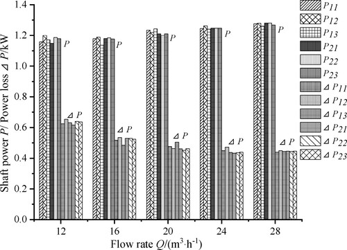
Figure 8 illustrates the histogram of the shaft power and the power loss for different impellers. The variation of the shaft power with the flow rate of six impellers is similar in the whole operating range. The shaft power increases with the flow rate. When the blade inlet angle varies, the shaft powers of the three impellers in Group 1 are significantly affected. Notably, the consumed shaft power of impellers11, 12, and 13 at the design condition are higher than those of impellers 21, 22, and 23, respectively. The corresponding difference between them is 24, 9, and 33 W, respectively. Moreover, the power loss against flow rate has almost a parabolic distribution. When the inlet angle changes, the power losses of the impellers in Group 1 change dramatically, whereas those of Group 2 change relatively gently. At the design condition, the power loss of the impeller in Group 2 is higher than that of Group 1. Power losses of impellers 11, 12 and 13 are 15, 12, and 43 W higher than those of impellers 21, 22, and 23, respectively. This finding is consistent with the results of the efficiency analysis in the foregoing section.

Figure 8. Histogram of shaft power and power loss for six impellers.

The relationship between the external characteristics of a single blade centrifugal pump and its blade inlet angle may be interpreted as follows. When the blade inlet angle increases, the blade bending is reduced, thereby expanding the blade inlet flow area. Therefore, pump head and efficiency are improved. On the other hand, given that a single blade centrifugal pump has only one blade, the capability of the pump on the fluid delivery is weakened, and thus pump head and efficiency decreases. The ultimate increase or decrease in pump head and efficiency depends on the strength of the foregoing two conditions. First, the blade streamline inlet angles of impellers 11, 12, and 13 increase from the front shroud to the rear one, thereby causing the impeller channel to diffuse and generate vortices. Thus, the efficiency of the three impellers is slightly lower than that of impellers 21, 22, and 23, respectively. This finding can be confirmed in Figure 10(a’,b’). That is, the fluctuation of the relative velocity on the streamline of the pressure surface of impellers in Group 1 is more serious than that of Group 2.

4.2. Flow field analyses

Figure 9 depicts the relative velocity contour distribution for six impellers at mid-span under the design condition (Q_d=20 m³/h). The relative velocity distributions of the six impellers are similar. Low velocity exists at the partial blade pressure/suction surface, the blade inlet, and near the tongue, and it reaches the maximum at the blade outlet. For the six impellers, a wake flow at the blade outlet.

Figure 9. Relative velocity contour distributions for six impellers under the design condition.

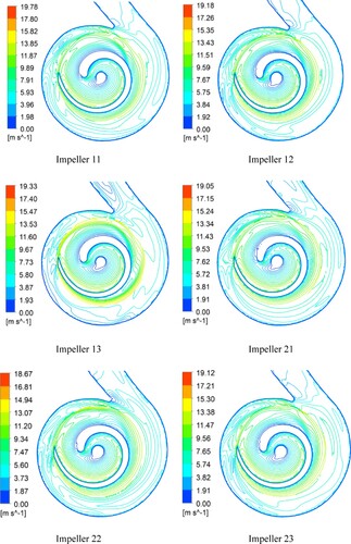
Figure 10 shows the relative velocity distribution curves of the blade pressure surface and suction surface streamlines at mid-span under the design condition. In Figure 10, the circumferential angle is plotted on the abscissa. Considering that the blade wrap angle is 360°, the blade inlet is set to 0°, and the blade outlet is set to 360°. Figure 10(a) shows the changes in the relative velocity from 0° to 11.25° for the middle streamline on pressure surface and suction surface of the impellers in Group 1. Figure 10(b) presents the impellers in Group 2. The range from 0° to 11.25° is exactly around the blade leading edge. Figure 10(a’,b’) shows the changes of the two above variables from 11.25° to 360°. After the fluid enters into the impeller, it circumvents the blade leading edge. After a short distance, the relative velocity on the streamline of the blade pressure surface (w_p) reaches the maximum value (the relative velocity can be considered to reach its maximum value at 0°) and then decreases to the minimum value at approximately 80°. Subsequently, although the relative velocity fluctuates, it generally increases until the impeller outlet is reached. w_p of impeller 13 fluctuates the most seriously. This phenomenon may be the reason why impeller 13 has the lowest efficiency under the design condition. Figure 10 shows that w_p suddenly decreases at about 160°, and the region from 0° to 160° is where fluid separation occurs on the blade pressure surface in Figure 9. Further analysis shows that w_p of impellers in Group 2 is larger than those of in Group 1 at 0°. Moreover, w_p of the impellers in the two groups approximately decreases to the same value at the same position (80°). That is, the velocity gradient of the impellers in Group 2 is larger than that of in Group 1. Therefore, as shown in Figure 9, the flow separation of impellers in Group 2 at the front of the blade pressure surface is more serious than that of impellers in Group 1.

Figure 10. Relative velocity distribution curves of the middle streamline on the pressure/suction surface

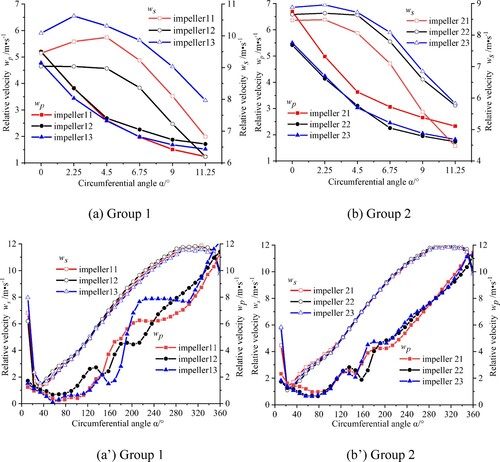
In Figure 10, very high velocities are generated on the suction surface of the blade leading edge because of the flow around the blade leading edge. w_s is the relative velocity on the streamline of the blade suction surface. In the range of 0° to 20°, w_s of impeller 21 is smaller than that of impeller 11. Thus, the pressure of the former is higher than that of in the latter (Figure 9). The same is true for impellers 23 and 13. Similarly, for impellers 12 and 22, the difference of w_s between them is very small; hence, the pressure difference is also very minimal. Furthermore, because of the thickness of the impeller blade trailing edge, the wake flow is observed at the blade outlet. The wake at the blade outlet is related to the velocity difference between the blade pressure surface and the suction surface here. The greater the velocity difference is, the more significant the wake is. In Group 1, impeller 11 has the smallest velocity difference, and impeller 22 is the smallest one in Group 2. In summary, the relative velocity distributions of impellers 11 and 22 are the most uniform in Groups 1 and 2, respectively.

Figure 11 shows the pressure distribution of six impellers at mid-span under the design condition. According to Figures 9 and 10, the pressure distribution of the impeller corresponds to its velocity distribution. For instance, when the relative velocity is high, the pressure is low, and vice versa. For the impellers in Group 1, the high-pressure range decreases with the increase in blade inlet angle. Moreover, the low pressure at the blade inlet first increases and then decreases as the blade inlet angle rises. Although the low-pressure region in impeller 13 decreases, negative pressure appears at the blade inlet. For clarification, the negative pressures are lower than the water vapor pressure (3.17kPa) at the standard atmospheric condition. Therefore, cavitation and corrosion easily occur at the suction surface near blade inlet. Meanwhile, for the impellers in Group 2, the minimum pressure first decreases and then increases, and no negative pressure occurs. Compared with impeller 13, the high-pressure range in impeller 23 rises. More specifically, the minimum pressure increases from −1.08 kPa to 9.83 kPa. Similarly, for impellers 11 and 21, the minimum pressure value increases from 4.02–10.2 kPa, whereas the minimum pressure value has a minimal difference for impellers 12 and 22. Therefore, for the impellers in Group 2, the possibility of cavitation is low at the lowest pressure area.

Figure 11. Pressure distributions in six impellers under the design condition.

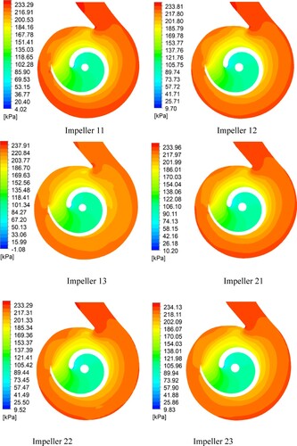
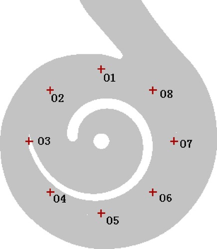
Figure 12 shows the positions of points O1–O8 at the impeller outlet. Points O1–O8 divide the impeller outlet into eight equal parts. The circumferential angle of point O1 is set to 0°. Consistent with the direction of rotation of the impeller, the circumferential angle of point O2 is set to 45°. Therefore, the circumferential angles of points O3–O8 increase by 45° in turn.

Figure 12. Corresponding point to the circumferential angle of the impeller outlet.

The pressure circumferential distribution of the six impellers at the impeller outlet is presented in Figure 13. The pressure distributions of all impellers along the circumference are extremely non-uniform. Moreover, minimum and peak pressure values are found downstream and near the tongue, respectively. The non-uniformity of the impeller outlet pressure represents the mixing loss that occurred here. As the non-uniformity degree increases, the outlet flow becomes more disordered, and the loss of the mixing collision between the fluid in volute and the impeller outflow rises. The standard deviation of pressure is used to evaluate the corresponding fluctuations. The pressure standard deviations of impellers 11, 12, and 13 are 4.41, 4.23, and 6.02 kP, respectively. These standard deviations indicate that the mixing collision loss of impeller 12 is the minimum, whereas that of impeller 13 is the maximum. Moreover, the pressure standard deviation of impellers 21, 22, and 23 are 3.75, 3.79, and 3.69 kP, respectively. Meanwhile, the difference in their mixing collision losses is negligible. The mixed collision loss of impellers in Group 2 is lower than those of Group 1.

Figure 13. Pressure distribution along the circumferential direction. (a) Impeller 11, 12 and 13 (b) Impeller 21, 22 and 23.

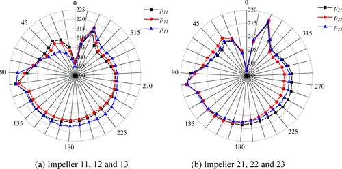
Figure 14 shows the relative velocity distribution at the impeller outlet. The relative velocity distributions of the six impellers are not remarkably uniform. As the non-uniformity degree increases, the flow becomes more disorganized at the outlet, and the energy exchange becomes more intense. Furthermore, the greater the relative velocity is, the lower the converted energy will be. The standard deviations of the relative velocity of impellers 11, 12, and 13 are 0.77, 0.78, and 0.88 m/s, respectively. On the other hand, the average relative velocities of the three impellers are 11.18, 11.40, and 13.25 m/s, respectively. Therefore, for the three impellers in Group 1, the adoption of a smaller blade inlet angle is beneficial to reduce the non-uniformity of the fluid flow at the impeller outlet, thereby improving the effect that impellers transform the fluid kinetic energy into pressure energy. The standard deviations of the relative velocity of impellers 21, 22, and 23 are 0.76, 0.89, and 1.00 m/s, respectively. The average relative velocities of the three impellers are 11.19, 11.07, and 11.26 m/s. The relative velocity of impellers in Group 2 is lower than that of Group 1, and the corresponding energy conversion degree of the former is higher than the latter. Meanwhile, the sudden expansion loss from the impeller to the volute can be reduced, whereas the relative velocity non-uniformity of impellers in Group 2 is slightly higher than that of Group 1. For the two groups, the relative velocity fluctuates more seriously at the impeller outlet as the blade inlet angle increases. Obviously, the outlet relative velocity of impeller 13 is much greater than those of the other impellers.

Figure 14. Relative velocity distribution along the circumferential direction. (a)Impellers 11, 12 and 13 (b) Impellers 21, 22 and 23.

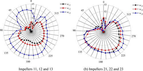
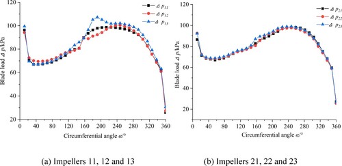
Figure 15 shows the blade load distribution for six impellers on the streamline at mid-span. The blade surface load refers to the pressure difference between the pressure surface and the suction surface at the same radius for the same blade. For Group 1, the blade load of impeller 11 changes relatively flat, whereas that of impeller 13 changes abruptly at approximately 200°. Flow separation is the reason for the sudden change in blade load. For Group 2, the blade load distribution of the three impellers is very similar, and no sudden change is observed in the blade load. For the two groups, Figure 12 shows that the blade load distribution of the impellers in Group 2 is flatter than those of Group 1. Therefore, the internal flow of the impellers in Group 2 is more uniform, and the alternating load is small on the blades, which does not cause fatigue failure easily.

Figure 15. Blade load distribution on the middle streamline.(a) Impellers 11, 12 and 13 (b) Impellers 21, 22 and 23.

5. Experimental validation

An open pump test rig is set up in the Jiangsu University (China) to verify the accuracy of the calculation (Figure 15). The WT2000 pressure transmitters are applied to measure the inlet and outlet pressures with the accuracy of ±0.1%. Moreover, the LWGY-50A turbine flow meter is applied to obtain the amount of fluid through the pump with the precision of ±0.5%.

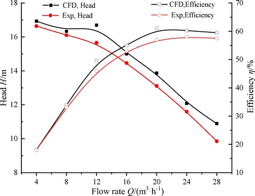
Impeller 12 is selected as the test impeller. The performance curves of the model pump are shown in Figure 16. The efficiencies of the numerical computation are higher than those for the experiment. The difference between the numerical and experimental results may come from the ignored various losses in the numerical simulation. However, the numerical and experimental results show similar trends. Compared with the experimental data, the maximum relative errors of the pump head is 6.6%, except for the flow rate of 28m³/h, and the maximum relative errors of efficiency is 7.8%. Therefore, the numerical results have an acceptable accuracy (Figure 17).

Figure 16. Open pump test rig.

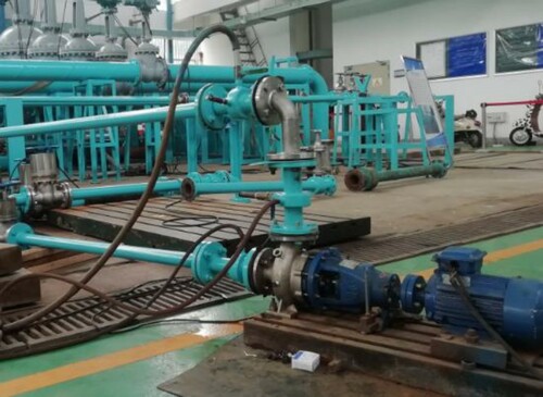
Figure 17. Performance curves of the model pump.

6. Conclusion

The relationship between the blade inlet angle and the behavior of the single blade centrifugal pump is investigated on the basis of CFD simulation and experiment results. The following conclusions are drawn on the basis of the aforementioned analyses:

1. In comparison with the three impellers of Group 2, the head and shaft power of the three impellers in Group 1 are more sensitive to the blade inlet angle. The distribution of the efficiency curve versus the flow rate for Group 2 impellers is almost flat. Blade inlet angle has an evident influence on the pressure and velocity distribution. The present results show that impeller 11 in Group 1 and impeller 22 in Group 2 have the best performance.

2. The blade inlet angle has a great influence on the first quarter of the blade pressure surface and the fluid recirculation at the blade inlet. For the three impellers in Group 1, the relative velocity on the last of streamline of the blade pressure surface fluctuates seriously. Moreover, the alternating load is large on the blades of the three impellers in Group 1.

3. The analysis of the distributions of pressure and velocity suggests that the energy conversion ability of impellers in Group 2 are higher than that of Group 1. For the studied impellers, the use of an impeller with a decreasing inlet angle from the front shroud to the rear one is recommended.

4. Considering that the present blade is a twisted blade, the blade manufacturing accuracy is not in agreement with the expected one. Therefore, the error between the calculated and the experimental results seems to be slightly huge. The inner flow mechanism, the appearance of radial force, and the noise of the single blade centrifugal pump are promising research directions in the future.

Disclosure statement

No potential conflict of interest was reported by the authors.

Additional information

Funding

This work was supported by the National Natural Science Foundation of China [Nos 51979138 and 51776087].

References

- Abadi, A. M., Sadi, M., Farzaneh-Gord, M., Ahmadi, M.H., Kumar, R., &Chou, K.W. (2020). A numerical and experimental study on the energy efficiency of a regenerative heat and mass exchanger utilizing the counter-flow Maisotsenko cycle. Engineering Applications of Computational Fluid Mechanics, 14(1), 1–12. https://doi.org/https://doi.org/10.1080/19942060.2019.1617193
- Aoki, M. (1984). Instantaneous inter blade pressure distributions and fluctuating radial thrust in a single-blade centrifugal pump. Bulletin of JSME, 27(233), 2413–2420. https://doi.org/https://doi.org/10.1299/jsme1958.27.2413
- Benra, F. K., & Dohmen, H. J. (2008). Investigation on the time-variant flow in a single blade centrifugal pump. Proceedings of the 5th WSEAS International Conference on Fluids Mechanics (Fluids 08), 629–634.
- Benra, F. K., Dohmen, H. J., & Sommer, M. (2005). Periodically unsteady flow in a single-blade centrifugal pump numerical and experimental results. Proceedings of ASME Fluids Engineering Division Summer Meeting. Houston,USA, 1, 1223–1231.
- De Souza, B., Niven, A., & Daly, J. (2008). Single-blade impeller development using the design of experiments method in combination with numerical simulation. Proceedings of the Institution of Mechanical Engineers, Part E: Journal of Process Mechanical Engineering, 222(3), 135–142. https://doi.org/https://doi.org/10.1243/09544089JPME218
- De Souza, B., Niven, A., & Mcevoy, R. (2010). A numerical investigation of the constant- velocity volute design approach as applied to the single blade impeller pump. Journal of Fluids Engineering, 132(6), 1–7. https://doi.org/https://doi.org/10.1115/1.4001773
- Ghalandari, M., et al. (2019). Investigation of Submerged Structures’ Flexibility on Sloshing Frequency using a boundary element method and finite element analysis. Engineering Applications of Computational Fluid Mechanics, 13(1), 519–528. https://doi.org/https://doi.org/10.1080/19942060.2019.1619197
- Guan, X. F. (2011). Theory and design of modern pump. China Astronautic Publishing House.
- Michael, H., Kuhimann, J., & Benra, F. K. (2009). Designing high-power sewage water pumps. World Pumps, 514, 20–25.
- Nishi, Y., Fujiwara, R., & Fukutomi, J. (2009). Design method for single blade centrifugal pump impeller. Journal of Fluid Science and Technology, 4(3), 786–800. https://doi.org/https://doi.org/10.1299/jfst.4.786
- Nishi, Y., Makita, K., & Fukutomi, J. (2006). A study on a new type of sewage pump. Nippon Kikai Gakkai Ronbunshu B Hen(Transactions of the Japan Society of Mechanical Engineers Part B (Japan), 72(720), 1984–1992.
- Pei, J., Dohmen, H. J., & Yuan, S. Q. (2012a). Investigation of unsteady flow-induced impeller oscillations of a single-blade pump under off-design conditions. Journal of Fluids and Structures, 35, 89–104. https://doi.org/https://doi.org/10.1016/j.jfluidstructs.2012.08.005
- Pei, J., Yuan, S. Q., & Dohmen, H. J. (2012b). Numerical prediction of unsteady pressure field within the whole flow passage of a radial single-blade pump. Journal of Fluids Engineering, 134(10), 1–11. https://doi.org/https://doi.org/10.1115/1.4007382
- Pei, J., Yuan, S. Q., & Yuan, J. P. (2013). Numerical analysis of periodic flow unsteadiness in a single-blade centrifugal pump. Science China Technological Sciences, 56(1), 212–221. https://doi.org/https://doi.org/10.1007/s11431-012-544-x
- Peng, G., Huang, X., Zhou, L., Zhou, G., & Zhou, H. (2020). Solid-liquid two-phase flow and wear analysis in a large-scale centrifugal slurry pump. Engineering Failure Analysis, 114, 104602. https://doi.org/https://doi.org/10.1016/j.engfailanal.2020.104602
- Salih, S. Q., Suliman, M., Rasani, M.R., Ariffin, A.K., & Yaseen, Z.M. (2019). Thin and sharp edges bodies-fluid interaction simulation using cut-cell immersed boundary method. Engineering Applications of Computational Fluid Mechanics, 13(1), 860–877. https://doi.org/https://doi.org/10.1080/19942060.2019.1652209
- Tan, L. W., Shi, W. W., & Zhang, D. S. (2018). Experiment on fluid force induced vibration for centrifugal pumps. Transactions of the Chinese Society for Agricultural Machinery, 49(5), 179–185. https://doi.org/https://doi.org/10.6041/j.issn.1000.1298.2018.05.020
- Tan, L. W., Shi, W. D., Zhang, D. S., Zhang, Y., & Zhang, W. Q. (2017). Effects of blade outlet angle on performance for single blade pumps. Journal of Drainage and Irrigation Machinery Engineering, 35(10), 835–855. https://doi.org/https://doi.org/10.3969/j.issn.1674-8530.16.0235
- Wang, H., Long, B., Wang, C., Han, C., & Li, L. (2020). Effects of the impeller blade with a Slot structure on the centrifugal pump performance. Energies, 13(7), 1628. https://doi.org/https://doi.org/10.3390/en13071628
- Wang, H., Long, B., Yang, Y., Xiao, Y., & Wang, C. (2020). Modelling the influence of inlet angle change on the performance of submersible well pumps. International Journal of Simulation Modelling, 19(1), 100–111. https://doi.org/https://doi.org/10.2507/IJSIMM19-1-506
- Zhou, L., Han, C., Bai, L., Li, W., El-Emam, M., & Shi, W. (2020). CFD-DEM bidirectional coupling simulation and experimental investigation of particle ejections and energy conversion in a spouted bed. Energy, 118672. doi:https://doi.org/10.1016/j.energy.2020.118672