
 ?Mathematical formulae have been encoded as MathML and are displayed in this HTML version using MathJax in order to improve their display. Uncheck the box to turn MathJax off. This feature requires Javascript. Click on a formula to zoom.
Abstract
The efficient removal of material debris by flushing is critical for the performance and the surface quality of the electrical discharge machining (EDM) manufacturing process. The particle concentration alters the thermal, mechanical, and electrical properties of the particle–dielectricum suspension and affects the manufacturing process and the surface quality by inducing high thermal loads. For the first time, we perform a direct particle–fluid simulation of the flushing cycle in a generic EDM cavity using a hierarchical Cartesian sharp-interface cut-cell method. The flow around each debris particle is completely resolved and the heat transfer between the particles and the fluid is taken into account. The rate of material removal and the cooling performance of the flushing mechanism are studied for three-volume loadings. The results show that the flow around the particles has a pronounced impact on the heat transfer between the dielectricum and the workpiece. A particle loading of 14% increases the mean heat transfer by approximately 16%. The particle loading also has a pronounced impact on the rate at which particles are flushed out of the cavity. Increasing the initial volume loading from 6% to 14% decreases the amount of particles that get flushed out of the cavity by 14%.
1. Introduction
Electrical discharge machining (EDM) (Singh et al., Citation2004) is a manufacturing process frequently used in the automotive, aerospace, microelectromechanical systems (Michel et al., Citation2000; Uhlmann et al., Citation1999), and bio-medical industry (Ho & Newman, Citation2003). It produces high-quality surfaces while allowing precise material removal. The process shapes a workpiece using a large number of high-frequency electrical discharges produced by an electrode submerged in a liquid insulating dielectricum under the action of an electric current. After removal, the material solidifies in the form of very small spherical hollow particles with a diameter in the range of depending on the process parameters (Haas et al., Citation2013; Murray et al., Citation2016). The particle concentration alters the thermal, mechanical, and electrical properties of the particle–dielectricum suspension and affects the manufacturing process and the resulting surface quality by inducing high thermal loads (Kumar et al., Citation2009). The heat transfer between the workpiece and the fluid is responsible for the temperature distribution in the workpiece's rim zone and critical for the resulting surface integrity. That is, due to thermal expansion effects, the heat flux defines the machining precision and is to be determined in detail to evaluate the EDM process. This study focuses on die-sink EDM where the material is removed in a small cavity within the workpiece. The stability of the process is dominated by the capacity of the flushing mechanism to cool the electrode and the workpiece and to pump the removed material through the lateral gaps of the electrode out of the cavity (Goodlet & Koshy, Citation2015; Uhlmann et al., Citation2005). Therefore, the die-sink EDM process uses a hybrid cycle with two phases: (I) a material removal phase in which the workpiece is eroded by a large number of high-frequency sparks and (II) a flushing phase in which the particles generated from the eroded material are flushed out from the working cavity. In the pressure flushing technique, the fresh dielectricum is pumped through a drilled machining electrode right into the cavity, to remove the material symmetrically through the lateral gap between the electrode and the workpiece. The lateral gap thicknesses between the electrode and the workpiece and the cavity depth are on the order of
. These small gaps combined with the geometrical constraints of the problem and the physical properties of the EDM process, i.e. intensive electrical discharges with small time scales, make measurements of the particle–laden flow in the working cavity extremely challenging. Therefore, primarily numerical simulations were conducted to study the flushing mechanisms in EDM. Haas et al. (Citation2013) performed numerical simulations of the fluid flow in wire-cut EDM using the Reynolds-Averaged Navier–Stokes (RANS) equations of a two-dimensional single-phase fluid to optimize the design of flushing nozzles. The analysis resulted in significant improvements of the cooling efficiency and wire stability of the process. The fluid flow induced by single electrical discharge was simulated by Shabgard et al. (Citation2013) using a RANS method to study how the pulse time affects the flushing efficiency of molten material. Z. Wang et al. (Citation2018) used steady two-dimensional axisymmetric simulations to develop a flushing mechanism that combines electrode-internal with electrode-external flushing and significantly improves the process efficiency by reducing the material debris concentration in the machining gap. Kliuev et al. (Citation2018) performed three-dimensional RANS simulations using the k-ϵ turbulence model to evaluate the flushing efficiency of multi-channel electrode configurations in deep hole drilling.
Two-phase RANS simulations were performed by Xu et al. (Citation2015) and Ji et al. (Citation2013) to evaluate the performance of new flushing mechanisms. Xu et al. (Citation2015) designed a multi-hole electrode with variable hole diameter, where the numerical simulations were used to optimize the diameter distribution and evaluate the performance of the electrode with respect to the produced material removal rate. Ji et al. (Citation2013) simulated a new hybrid coaxial-orbital flushing technique and the material removal rate performance was evaluated against that of non-hybrid coaxial and orbital methods. Liu et al. (Citation2018) studied the impact of ultrasonic electrode vibrations on the flushing of material debris from the machining gap using three-dimensional fluid simulations with a Lagrangian-particle model. The influence of the gas-bubble dynamics on the material removal and its role on the cavity flow field of the EDM process were analyzed by J. Wang and Han (Citation2014) using a three-phase RANS approach. Recently, the heat transfer and the heat dissipation rate of the dielectric fluid were investigated by Das et al. (Citation2019) using a three-dimensional fluid simulation with a state-of-the-art bubble-dynamics model that takes material vaporization into account. The erosion, ejection, and solidification processes in EDM were simulated by Zhang et al. (Citation2019). Modeling the heat flux density, vapor flow, and the stages of the eroded material prior to particles, i.e. melting, ejection, and solidification, the EDM process of a single–pulse discharge experiment could be analyzed.
Note that these studies and numerous other analyses of the flushing cycle found in the literature are based on the RANS approach. That is, the accuracy of the results relies on turbulence models developed for aerodynamic slender body flows over smooth surfaces. However, in the analysis of EDM flushing impinging jets, boundary layer separation, and complex vortical structures occur. Furthermore, the application of one-way coupling between fluid and particles is an extremely simple model since it does not account for the interaction between the phases (Elghobashi, Citation1994). Even the Euler–Lagrange approach for multi-phase models determines an uncertainty since a fundamental condition that has to be satisfied by the numerical method for such analyses is the conservation of mass, momentum, and energy at the particle–fluid interface. Euler-Lagrangian techniques are generally not well suited, since to satisfy the geometric conservation law expensive and continuous remeshing is required due to the arbitrarily large particle displacements which are not known a priori. Non-boundary conforming methods avoid remeshing by superimposing the particle geometry on a background mesh (Saliha et al., Citation2019). In the original immersed boundary method (Peskin, Citation1972), the effect of the moving boundaries on the flow is simulated by a discrete forcing term in the momentum equation. The known jumps across the interface are taken into account via correction terms in the numerical discretization (Z. Li & Lai, Citation2001). This approach, however, suffers from being not strictly conservative and smearing the sharp interface over several cell layers. A superior approach to overcome the limits of modeling are direct particle–fluid simulations (DPFS).
Direct particle–fluid simulations, i.e. numerical simulations of multi-phase flows in which turbulence and the flow field around each particle are fully resolved, are computationally a challenging multi-physics multi-scale problem when the particle diameter is in the range of the Kolmogorov length scale (Balachandar & Eaton, Citation2010). Schneiders et al. perform DPFS to investigate particle–laden isotropic turbulence for particle and turbulence parameters that forbid any modeling approach (Schneiders et al., Citation2019, Citation2017a, Citation2017b). They developed and used a massively parallel (Lintermann et al., Citation2014) adaptive hierarchical Cartesian cut-cell method (Hartmann et al., Citation2011) for multi-phase flows (Meinke et al., Citation2013; Schneiders et al., Citation2016) and complex geometries (Günther et al., Citation2014).
Based on the method by Schneiders et al. (Citation2017a), we perform DPFS of the mono-hole pressure flushing flow in a generic die-sink EDM cavity, i.e.the flow around each debris particle is fully resolved and the heat transfer between the particles and the fluid is also taken into account. Hence, the effect of the particle-particle interaction in the dielectricum and the fluid–particle interactions are accounted for. We address the question whether fluid–particle interactions can be neglected or should be modeled in the numerical analyses of the EDM flushing cycle to predict the thermal loads that need to be sustained by the workpiece. The necessity of incorporating the debris particles in numerical simulations of the flushing cycle of EDM is studied by quantifying their impact on the total heat exchange.
The paper is organized as follows. In Section 2, the generic die-sink EDM cavity and the mathematical model to describe the multi-phase flow are introduced. In Section 3, the numerical method is presented. Then, the results are discussed in Section 4 and finally, some conclusions are drawn in Section 5.
2. Mono-hole pressure flushing in die-sink EDM
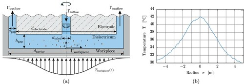
The generic axisymmetric die-sink EDM cavity is schematically shown in Figure (a), in which the cavity geometry and boundary conditions of the problem are described. A cut through the drilled electrode, depicted by dashed lines, reveals the single pipe-like hole of diameter through which the fresh dielectricum enters the cavity. The cylindrical cavity has a diameter
, a height
, and is initially filled with a particle suspension at rest. The particle–laden fluid exits the system through the lateral cylindrical gap of thickness
between the electrode and the workpiece. On the bottom boundary between the fluid and the workpiece, a temperature distribution is used to model the latent heat stored in the workpiece during the material removal phase of the EDM process.
Figure 1. (a) Axisymmetric geometry of the die-sink EDM cavity including boundary notations. (b) Axisymmetric temperature distribution from thermographic camera measurements (Brito Gadeschi, Schneider, et al., Citation2017).
Next, the mathematical model to describe the two-phase fluid flow is introduced. This includes the model for the unsteady flow, the rigid body particle dynamics, the heat transfer between the particles and the fluid, and the boundary conditions. The parameters of the fluid and the solid particles are given in Tables and in Section 4.
2.1. Mathematical model
This section briefly introduces the mathematical model used to describe the physics of the two-phase solid–fluid flow in the EDM gap once all gas bubbles created by the electrical discharges have left the cavity, i.e. a third gaseous phase is not considered in this study. The Navier–Stokes equations are used to describe the motion of the fluid, whereas the debris particles are modeled as rigid spheres.
2.1.1. Navier–Stokes equations
The integral non-dimensional form of the unsteady conservation equations of mass, momentum, and energy for a moving control volume reads
(1)
(1) The conserved quantities
are defined by the density ρ, pressure p, velocity vector
, and specific total energy E. The nonlinear flux vector
(2)
(2) Reynolds number
, shear stresses
, and heat flux
. The quantity
denotes the velocity of the control volume. Since the fluid can be considered to be incompressible, a low Mach number of M = 0.1 is assumed. Further information on the governing equations can be found in Brito Gadeshi, Schneiders, et al. (Citation2017) and Schneiders et al. (Citation2017a, Citation2017b).
2.1.2. Boundary conditions
The boundary conditions for the inflow, outflow, and solid wall boundaries are introduced next. Let Γ denote a boundary surface, the inflow boundary condition on is given by
(3)
(3) where
is the vector normal to the boundary surface pointing inside the fluid domain. The quantity
is the radial coordinate of the cylindrical coordinate system shown in Figure (a). The axisymmetric parabolic laminar velocity profile
prescribed at the inflow reads
(4)
(4) where the maximum velocity at r = 0 is
. The maximum velocity is
using the rectangular function χ that is
for
and
otherwise. The mass flow is
(5)
(5) On the outflow boundary
,
(6)
(6) are prescribed. The pressure is defined by the hydrostatic pressure
at the outflow of the lateral cylindrical gap. On the bottom of the cavity
, a no-slip boundary condition with a prescribed temperature distribution
(7)
(7) is imposed, where the pressure is determined by the approximation of a vanishing normal gradient. The surface temperature
on the workpiece which is sketched in Figure (a) is obtained from thermographic camera measurements by Brito Gadeschi, Schneider, et al. (Citation2017) the distribution of which is shown in Figure (b). It is prescribed using a steady Gaussian temperature profile with a peak temperature
.
2.2. Heat-conducting moving solid particles
The debris particles are modeled as rigid spheres of diameter and their boundary denoted by
is illustrated in Figure (a). First, the governing equations are briefly discussed. Then, the boundary conditions are defined.
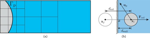
Figure 2. (a) Exemplary two-dimensional hierarchical Cartesian grid in which the cells intersected by the particle–fluid interface are reshaped to conform to the moving boundary. (b) Modeling of the collision between the particle i and a solid wall at distance
using a mirror particle j such that the short-range repulsive force
points in the wall-normal direction towards the particle i.
2.2.1. Governing equations
The governing equations of translational and rotational motion are
(8)
(8)
(9)
(9) with the particle mass m, the particle velocity
, the hydrodynamic force
, the collision force
, the gravitational acceleration
, the moment of inertia
, the angular velocity
, and the hydrodynamic torque
. That is, the particles move in response to the fluid forces and alter the flow field, which in turn changes the fluid forces acting on the particles. Hence, a fully coupled fluid-structure interaction problem is considered.
Furthermore, the particles exchange heat with the embedding fluid altering the particle temperature . The change of
is modeled using a first-order approach for small particles
(10)
(10) The material parameters of the particle density
, specific heat capacity
, and thermal conductivity
are listed in Table . Further computational details can be found in Brito Gadeshi, Schneiders, et al. (Citation2017) and Schneiders et al. (Citation2017a, Citation2017b).
2.2.2. Boundary conditions
The momentum and energy exchange between the particle and the fluid is prescribed using the following boundary condition for the fluid phase on the particle boundary
(11)
(11)
2.3. Initial condition
The flow field for a quiescent fluid is initialized by ,
, and
. Initially, the particles are at rest and the particle temperature equals the maximum temperature obtained from the thermographic camera measurements by Brito Gadeschi, Schneider, et al. (Citation2017). The particles are distributed homogeneously and axisymetrically at a distance of one
over the cavity bottom surface.
3. Numerical method
The cut-cell finite-volume method used in this work is a conservative multi-phase method for compressible flows (Hartmann et al., Citation2008, Citation2011) that has been extended to moving boundary problems (Schneiders et al., Citation2016, Citation2013), complex moving boundaries (Günther et al., Citation2014), and massively parallel computing (Lintermann et al., Citation2014). It has been successfully applied to study particle–laden flows using Euler–Lagrange (Siewert et al., Citation2014) and fully resolved particle models (Schneiders et al., Citation2019, Citation2017a, Citation2017b). In Brito Gadeschi et al. (Citation2015) and Brito Gadeshi, Schneiders, et al. (Citation2017), also the heat transfer between particles and fluid is taken into account. As for direct-numerical simulations (DNS) of single-phase flows, all scales of particle–laden flows are resolved in the DPFS, i.e. no turbulence modeling is used. A brief description of the numerical method, i.e. the spatial discretization, the temporal integration, and the representation of particles, is given in the remainder of this section.
The fluid equations described in Section 2.1 are solved on an unstructured hierarchical Cartesian mesh (Schneiders et al., Citation2016). For the spatial discretization of the inviscid flux terms an advection upstream splitting method (AUSM) is used (Liou & Steffen, Citation1993; Meinke et al., Citation2002). The viscous flux is discretized by central differences.
The boundary of the particles in Figure (a) is described by a level-set function on the hierarchical Cartesian grid (Osher & Sethian, Citation1988). The function is the scalar field of the shortest distance between point
and the particle surface
. The level-set field is computed analytically using the particle position
and the radius
(Günther et al., Citation2014). The fluid cells intersected by the solid boundary are reshaped to yield a linear boundary representation. The pressure and stress forces are integrated over the boundary of the fully resolved particles and the right-hand side of Equations (Equation8
(8)
(8) ) and (Equation9
(9)
(9) ) are determined to move the particles. Analogously, the heat flux is computed to integrate Equation (Equation10
(10)
(10) ). The forces of particle–particle and particle–wall collisions
in Equation (Equation8
(8)
(8) ) are based on a model by Glowinski et al. (Citation1999) illustrated in Figure (b). For the latter case, a mirror image of the particle outside the physical domain is considered such that the direction of the short-range repulsive force is normal to the solid wall.
The heat flux in Equation (Equation10
(10)
(10) ) is based on Fourier's law and the temperature difference between the particle and the surface of the particle. While the particle temperature
represents an average, the temperature at the surface of the particle is defined by the local boundary conditions at
.
For the temporal integration of the flow field governed by Equation (Equation1(1)
(1) ) and the particle motion described by Equations (Equation8
(8)
(8) ) and (Equation9
(9)
(9) ), a 5-stage Runge–Kutta scheme is used (Schneiders et al., Citation2016). The predictor–corrector scheme ensures stability up to a Courant–Friedrichs–Levy (CFL) number of 4. In this study, the CFL numbers for the inviscid and viscous terms are
and
.
4. Results
The numerical method has previously been validated for multi-phase flows (Schneiders et al., Citation2016, Citation2017a) and conjugate heat transfer (Brito Gadeschi et al., Citation2014, Citation2015). In the following, first, the single-phase formulation of the numerical method is validated for an internal flow problem and the accuracy of the particle–wall collision model is assessed. Next, the heat transfer and particle transport of mono-hole pressure flushing is analyzed. The single-phase flushing flow is studied first, and then these results are compared against the particle–laden flushing flow.
4.1. Channel flow
The findings of the single-phase formulation of the numerical method for channel flow are compared with the direct numerical simulation results of Moser et al. (Citation1999). The flow and numerical parameters are given in Table and the simulation setup is shown in Figure . The quantity H is the channel height, the channel length, and W = 1.75H the cannel width. Symmetry boundary conditions are used on the lateral sides of the channel and the inflow bulk velocity
and the outflow pressure
are prescribed according to the pressure gradient required to obtain
(Moser et al., Citation1999). The Mach number is M = 0.1 and the simulated time equals the time required for a fluid particle to traverse the channel length 27 times according to the fluid bulk velocity. The number of cells is approximately
and the number of time steps is 200,000.
Figure 3. Domain and boundary conditions of channel flow.
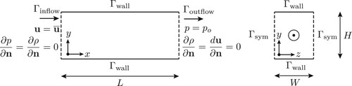
Table 1. Flow and numerical parameters for channel flow.
Table 2. Geometric, material, boundary and initial condition parameters for generic flushing-flow in die-sink EDM using mono-hole pressure flushing with the Oelheld IME-68 dielectric (Oelheld dielectrics, https://www.oelheld.com/).
The instantaneous -contours (Jeong & Hussain, Citation1995) colored by the streamwise velocity component in Figure illustrate the turbulent structures of the flow field. The root-mean-square (RMS) of the velocity components spatially averaged in the streamline and spanwise direction are shown in Figure (a). The temporal averaging was computed over 27 convective units. A good agreement with the results from Moser et al. (Citation1999) is obtained for
,
, and the turbulent shear stress
. A slight overshoot of
in the range
is observed. The shear balance in Figure (b) shows a minor deviation of the total shear stress τ in the range
. Finally, the comparison of the distributions of the streamwise velocity component
normalized by the friction velocity in Figure (c) shows an excellent agreement with the data of Moser et al. (Citation1999).
Figure 4. Instantaneous -contours colored by the non-dimensional streamwise velocity component
.
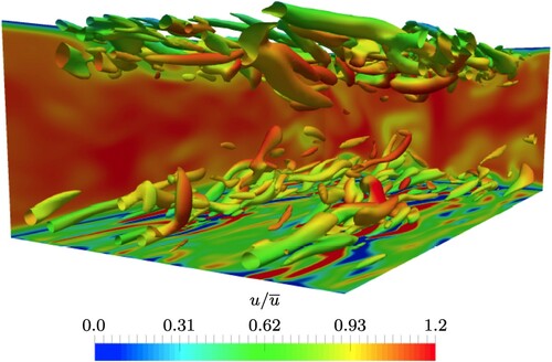
Figure 5. (a) Root-mean-square (RMS) distributions of the velocity components; (b) shear balance, laminar and turbulent shear stress, and
, and the total shear stress
; (c) streamwise velocity component
normalized by the friction velocity
on a semi-logarithmic scale.
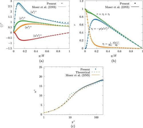
In conclusion, these results for the single-phase channel flow show a convincing match with the results of Moser et al. (Citation1999). The overshoot in and the deviations observed in the shear stress τ are small and can be attributed to the usage of different meshes between the current simulations and the reference. The findings demonstrate the validity of the method to accurately analyze internal flows such as EDM flushing.
4.2. Sphere–wall collision
The study of the dynamics of a sphere immersed in a viscous fluid impinging on a solid wall is an area of active research (Izard et al., Citation2014; X. Li et al., Citation2011). In this section, the results of the numerical method for particle-wall collisions based on Glowinski's model (Glowinski et al., Citation1999) are compared with findings from the literature. The experimental and numerical study of X. Li et al. (Citation2011) considers a configuration, ‘Case 7’, with a ratio of the particle density and the fluid density , which is on the same order of magnitude as the density ratio in the subsequent sections of this study (
).
The simulation setup is shown in Figure (a). The stationary solid wall is located at and free-stream boundary conditions are imposed on all other outer boundaries. The fluid is a mixture of Glycerol and water with a viscosity of
. The time is non-dimensionalized by
. The particle is initially at rest and its bottom is located at a distance of 3.75
above the wall and at rest. The impact Reynolds number is
. Note that the particle does not reach its terminal velocity before impact.
Figure 6. Impact of a sphere against a solid wall: (a) domain and boundary conditions; (b) computational grid; (c) comparison of the position of the particle bottom as a function of time
computed using the Glowinski model with the numerical results of X. Li et al. (Citation2011).
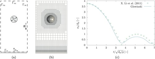
The three-dimensional computational domain is discretized using the adaptive hierarchical Cartesian grid is shown in Figure (b). The grid contains approximately 800,000 cells and the particle diameter is discretized by approximately 25 cells, that is, the smallest cell length is .
Figure (c) shows the distance between the particle bottom and the wall as a function of time . The time span in which the first two collisions with the wall occur is shown. The first collision occurs at t = 3.6 and the second one at
. During the initial fall, the Glowinski model results agree well with the experimentally calibrated numerical results of X. Li et al. (Citation2011) and the time instant at which the first collision with the wall occurs is captured by the scheme. Due to the grid in conjunction with the discretization, the Glowinski model starts repulsing the particle before the actual collision occurs, i.e. the particle's minimum distance to the wall is
which corresponds to 6.5 grid cells. Furthermore, the Glowinski model transfers less energy into the particle resulting in a smaller peak height at t = 5.1 after the first bounce.
Note that the collision model used by X. Li et al. (Citation2011) is computationally very costly and models the lubrication and elastic force terms with experimentally calibrated coefficients. For the purpose of this study considering EDM flushing, in which numerous particles and particle–particle and particle–wall collisions are considered, the simpler Glowinski model is a reasonable compromise between accuracy and computational efficiency.
4.3. Flushing flow
Next, the flow field in a generic die-sink EDM cavity using mono-hole pressure flushing described in Section 2 is studied. First, the geometric and flow parameters are introduced and an appropriate spatial discretization for the problem is defined. Then, the single-phase flow, i.e. the flushing flow without particles, is analyzed in Section 4.3.2. Subsequently, the particle–laden flushing flow is investigated and the single-phase and multi-phase flow results are compared in Section 4.3.3.
4.3.1. Geometry and flow parameters
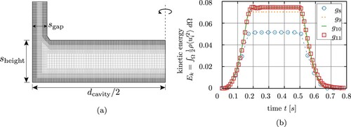
The parameters governing the geometry of the die-sink EDM cavity illustrated in Figure (left) are the cavity height and the cavity and electrode diameters
and
. The difference
defines the lateral gap of the cavity
. The aspect ratios between the lateral cavity gaps and the cavity diameter and between the cavity height and the cavity diameter are
and
.
Figure 7. (a) Radial axisymmetric slice of the hierarchical Cartesian grid ; (b) turbulent kinetic energy
of the fluid phase over time for the grids
.
The dielectric fluid Oelheld IME 68 is used. Its density and kinematic viscosity at are
and
. The Prandtl number of the flow is Pr = 23.4 and the Mach number is M = 0.1. The Reynolds number of the flow is
. A parabolic velocity profile with a maximum inlet velocity
is applied at the inflow boundary condition for a period of
, i.e. before
and after
the inlet velocity is zero. The fluid temperature at the inflow corresponds to the ambient temperature in the experiments,
C. These parameters are summarized in Table .
4.3.2. Single-phase flushing flow
Next, the mesh resolution for the flushing flow analysis is defined and the single-phase flow is investigated. A grid convergence study based on four grids is performed and the parameters of the grids are given in Table . A radial slice of the grid is shown in Figure (a). The parameters in Table are the length of the smallest isotropic Cartesian cell
, the total number of cells
, and the number of time steps to perform the simulation satisfying the stability constraints on the time step. The unstructured grids
have the same ‘pattern’ as that shown in Figure (a), i.e. every mesh is based on 4 levels. The subscript m in the mesh notation
denotes the number of isotropic refinements performed from an initial square Cartesian cell, which is large enough to encompass the whole computational domain, to the cell with the smallest cell length. That is, the smallest cell in
has twice the length as the smallest cell in
.
Table 3. The parameters of the spatial discretizations for the grid convergence study are the smallest cell length , the total number of cells
, and the total number of time steps
.
Table 4. Geometric, material, and initial condition parameters of the particles.
The criterion for the grid resolution study is the volume integrated turbulent kinetic energy
(12)
(12) which is shown as a function of time for each grid in Figure (b). The turbulent kinetic energy increases until
and remains constant until the jet is turned off at
. Then,
decays rapidly until
, where it achieves almost zero. Subsequently, the rate of dissipation is reduced and the kinetic energy continues to decay very slowly. A small amount of kinetic energy is still present in the flow at
.
The global temporal dynamics of the production, saturation, and dissipation of the kinetic energy is satisfactorily predicted by the meshes ,
, and
. However, only the two finest grids
and
hardly show any difference in the growth rate, the decay rate, and the plateau of the kinetic energy of the velocity fluctuations. Note that although the
resolution suffices, the grid
is used throughout this study.
The velocity magnitude and vorticity fields for 8 distinct time instants in the time interval are shown in Figures and . During the time interval
, the fluid is injected into the cavity. The inlet jet impinges upon the bottom of the cavity and generates a tip vortex and a stagnation flow. At
, the boundary layer extends over approximately
where also the weak tip vortex occurs. At the same time, large vortices form next to the core of the jet. While the fluid accelerates, vortex stretching occurs extending the structures to the lateral cavity gap at
. During vortex stretching, the boundary layer covering the cavity bottom interacts with the cylindrical cavity walls at
and a torus-like zone of recirculation occurs. The blockage caused by this recirculation decreases the cross-section to transport fluid and particles towards the lateral gaps. This narrow section causes the flow to be accelerated in the time interval
. The stream is surrounded by the vortex next to the jet and the zone of recirculation.
Figure 8. Velocity magnitude of the flushing flow at the time instants .
![Figure 8. Velocity magnitude of the flushing flow at the time instants t=[0.05 s,0.136 s,0.227 s,0.318 s,0.455 s,0.545 s,0.682 s,0.910 s].](/cms/asset/29b36c73-8330-4601-b29f-496dbd0b09c2/tcfm_a_1877198_f0008_oc.jpg)
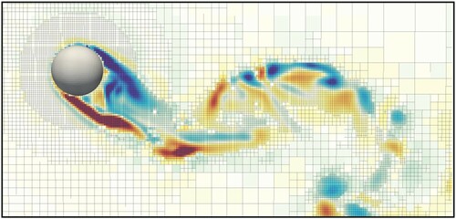
Figure 9. Nondimensional vorticity of the flushing flow at the time instants . Blue and red regions are counter–rotating.
![Figure 9. Nondimensional vorticity of the flushing flow at the time instants t=[0.05 s,0.136 s,0.227 s,0.318 s,0.455 s,0.545 s,0.682 s,0.910 s]. Blue and red regions are counter–rotating.](/cms/asset/384ac9bc-253e-4c97-a2eb-f5a099fc2467/tcfm_a_1877198_f0009_oc.jpg)
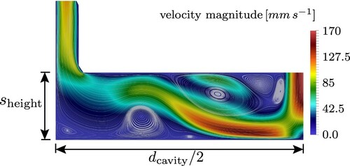
The structure of the jet and the recirculation region at can be observed in the streamlines of the projection of the velocity field in a two-dimensional cross section at
in Figure . It evidences that the recirculation region on the cavity bottom corner is formed by two small and elongated vortex cores at
and
and a larger core at
which grows till it reaches a height of
normal to the wall. The recirculation region on the electrode base is adjacent to the jet and also consists of three vortices. A large core at
and two small cores close to the jet at
and
occur.
Figure 10. Streamlines of the two-dimensional axisymmetric projection of the flushing flow at the time instant .
The heat flux through the workpiece surface controls the temperature in the rim zone. This distribution is critical for the resulting surface integrity and the machining precision of the electrical discharge machining process. The average heat flux per surface area between the solid and the fluid is determined by
(13)
(13) where
is positive in the wall-normal direction. That is, a positive heat flux denotes that heat is transferred from the solid into the fluid. The cooling effect of the single-phase flow on the workpiece is shown in Figure , where the average heat flux over a full flushing cycle is shown. The heat flux increases monotonically as the thin boundary layer shown in Figures and develops. When the recirculation region in the cavity corner begins to form at
, the area of the cavity bottom that interacts with the cold fluid stream decreases. The heat flux reduces slowly when the recirculation cores begin to form at
. This process is accelerated by the growth of the recirculation region. When the jet is turned off at
, the heat flux decays to approximately zero due to the dissipation of the kinetic energy.
4.3.3. Multi-phase flushing flow
In the following, the initial condition of the single-phase flushing flow is modified by introducing solid spherical heat conducting particles in the fluid. Three different volume loadings 6%, 9%, and 14% are studied. The particle diameter observed by Brito Gadeschi, Schneider, et al. (Citation2017) is which is of the same order of magnitude as the particle diameters observed by Tanjilul et al. (Citation2018). Since the total volume in the working gap is
, this results in 1500, 2300, and 3500 particles in the computational domain.
To quantify the influence of the material debris on the heat transfer through the workpiece during flushing, three homogeneous particle distributions corresponding to a volume loading of 6%, 9%, and 14% are studied. These volume loadings correspond to high material-removal rates in the range of
(Murray et al., Citation2016) which corresponds to a range from 1000 to 3500 particles. The particles are radially initialized at a distance of
over the cavity bottom surface. The heat transferred from the solid into the fluid during the solidification of the particles is taken into account by using an initial particle temperature of
C which corresponds to the maximum temperature obtained from the thermographic camera measurement shown in Figure (b). Although this initial particle temperature introduces a heat source in the initial condition that is not present in the single-phase flow case, the overall impact on the heat transfer through the workpiece is negligible.
The material parameters of the particles are listed in Table . The solid density is which corresponds to a solid-to-fluid density ratio
. The thermal conductivity and heat capacity of the particles
W/(m K) and
J/(kg K) are required to compute the heat exchange between the particles and the fluid.
The flow around the debris particles is resolved by adaptively refined mesh shown in Figure . The signed-distance field that captures moving boundaries is used to refine the grid around moving boundaries (Schneiders et al., Citation2016). Shear layers and steep velocity gradients are detected by the magnitude of the vorticity vector which drives the physics-based adaptation algorithm (Hartmann et al., Citation2008).
Figure 11. The adaptive mesh around a debris particle in regions of high vorticity. Blue and red regions are counter-rotating.
Next, the particle motion and the effect of the particles on the flushing flow are analyzed. Before the jet impinges on the cavity bottom, the temperature of the particles approximately takes on the local temperature of the fluid. It is shown in Figure that the particles are lifted-off the bottom of the cavity by the initial vortex tip and are transported out of the cavity through the fluid stream into the lateral gap. Figure illustrates the particle distribution for and
volume loading at the time instant
. The particles are colored by the temperature and their positions are projected onto a two-dimensional plane. In the cavity region near the axis, i.e. for the radius
, most particles have already been flushed away at
. The remaining particles in this region are located close to the electrode surface at the top of the cavity. These particles were lifted into this region by the tip vortex that is formed in the beginning of the flushing process and are trapped in the vortex ring between the surface of the electrode and the main flow. The pressurized jet continuously cools this region with fresh fluid and the particles attain a temperature of 20–22
. The temperature of the fluid above the main flow increases monotonously towards the lateral gap up to 25–26
. For both volume loadings, the particles located close to the workpiece surface possess a higher temperature of 35–36
in the area up to the radius
, where the prescribed workpiece temperature reaches
. The flow field underneath the main flow contains two recirculation regions centered at (I)
and (II)
. For both volume loadings, the particle temperature and particle distribution show these recirculation regions. However, for the larger volume loading 14%, the recirculation regions are more pronounced since there are more particles and their average temperature is higher. On average, the particle temperature of the second recirculation region is lower than that of the first for both volume loadings. Finally, the temperature of the particles in the main flow rises from
C at the center of the working gap to 28–29
in the lateral gap. In the lateral gap, the particle temperature decreases since the particles are flushed away due to the higher fluid velocity in the gap.
Figure 12. The fluid temperature (color map) and the particles (grey) located within a cylindrical region of radius of the domain at the time instant
.
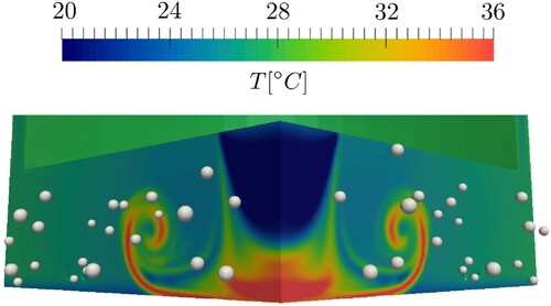
Figure 13. Planar projection of the particle distribution colored by the particle temperature for a volume loading of (a) 6% and (b) 14% at the time instant . (a) Volume loading 6% and (b) Volume loading 14%.
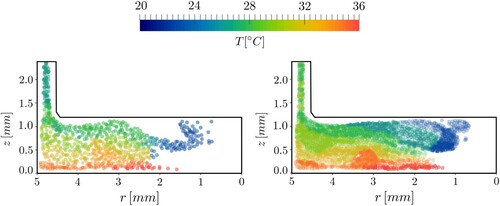
Figure 14. The distribution of the total heat flux on the surface of the workpiece as a function of time for the single phase flow and the three multi-phase flow cases.
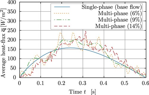
The effect of the particle loading on the spatially averaged heat flux (Equation13
(13)
(13) ) is shown in Figure . During the flushing of the cavity, positive values of the heat flux occur, i.e. the workpiece is cooled by the flow. The average heat flux through the cavity bottom of the three multi-phase flushing flow cases show a similar trend as that of the single-phase flow. Nevertheless, the distribution is significantly more perturbed. Initially, the heat flux increases up to the time
. During this phase, the average heat flux is lower than that of the single phase flow. This is due to the smaller temperature gradients that result from the heat released by the initially hot particles close to the cavity bottom. Due to their higher heat capacity, each solid particle stores the same thermal energy as an equivalent isothermal spherical fluid volume of radius
which has a three times larger volume. When this energy is released into the fluid, its temperature increases and reduces the heat flux through the cavity bottom. Depending on the volume loading, the heat flux reaches its maximum and plateaus in the time interval
. It oscillates strongly and shows a somewhat chaotic behavior. These oscillations result from increased heat transport in the recirculation regions containing entrained solid particles. Due to their higher heat capacity they are able to transport heat more efficiently into the main fluid stream since they are lifted up by the vortex cores. As the particles are flushed away from the cavity, the heat flux of all cases starts to converge. Finally, when the jet is turned off at
, the differences in the heat flux between the multi-phase and the single-phase flow are caused by the inertia of the particles in the recirculation regions which slow down the decay of total kinetic energy in the system.
To quantify the difference between the cases considered, the total average heat flux during the flushing cycle, i.e. the time integral of the surface averaged heat flux, is given in Table for the single-phase and the three multi-phase flow cases. The findings show that the solid particles have a pronounced impact on the heat flux through the workpiece. As the volume loading increases, the total heat flux increases with respect to the single-phase flow configuration.
Table 5. Total heat flux through a flushing cycle.
The particle removal statistics for a single flushing cycle of are provided in Table . Here,
is the total amount of particles flushed,
is their volume, and
is the volume of the initial amount of particles in the cavity. The findings show that the initial volume loading has a pronounced impact on the amount of debris flushed out of the cavity. As the initial volume loading increases, the amount of debris particles flushed
increases. However, this increase grows slower than the initial volume loading as shown by the ratio of the removed and initial volume loadings
, which decreases as the initial volume loading increases. That is, an increase in the initial volume loading from
to
reduces the relative amount of particles that are flushed from the cavity and therefore the efficiency of the flushing mechanism by
. This phenomena is caused by the constant surface area of the lateral cavity gap for which the particles need to compete for to escape from the cavity. Assuming a spacing of one particle diameter between the particles when exiting the gap, for the current configuration, the surface area of the lateral cavity gap is the same as that of 768 debris particles. This phenomena is observed in Figure (a) at the location where the lateral gap and the working gap meet, where the forming of a particle cluster characteristic for particle choking is found.
Table 6. Debris removal statistics: is the total number of debris particles removed during a flushing cycle,
is their volume, and
is the volume of the initial amount of particles in the cavity.
5. Conclusions
The efficient removal of material debris by flushing is critical for the performance and resulting surface quality of the electrical discharge machining (EDM) manufacturing process. In this study, a numerical model for quantifying the heat transfer between the workpiece and the flushing flow in a generic die-sink EDM cavity has been introduced. A hierarchical Cartesian cut-cell method that accounts for the fluid-particle heat transfer has been presented and applied to study the single-phase and multi-phase flushing flow in the generic EDM cavity by direct particle–fluid simulations. Three particle volume loadings have been considered. The analysis shows that the dynamics of the recirculation generates a high-speed stream which transports most of the fluid out of the cavity, while simultaneously creating recirculation regions in which particles are entrained. The comparison of the heat transfer from the workpiece into the fluid for the single-phase and the three multi-phase flow cases shows that the debris particles have a pronounced impact on the heat flux through the workpiece. To be more precise, a particle volume loading of 6%, 9%, and 14% increases the mean heat flux by 10%, 15%, and 16%. Furthermore, the analysis shows that the initial volume loading has a pronounced impact on the relative amount of particles that are flushed out of the working gap during a flushing cycle. Since the lateral gap surface remains constant, the particles choke trying to exit the cavity, reducing the overall efficiency of the flushing mechanism. Increasing the initial volume loading from 6% to 14% decreases the relative amount of particles that get flushed out of the cavity by 14%.
This study presents a fully resolved two-phase flow model to analyze the flushing flow in electrical discharge machining. This work is currently extended along two research directions, to experimentally validate the two-phase flow model presented in this work and to further develop the present method such that three-phase solid–fluid-gas flushing flows can be analyzed by fully-resolved simulations.
Acknowledgements
This work has been funded by the German Research Foundation (DFG) within the framework of the SFB/Transregio 136 ‘Process Signatures’ (subproject M04). This support is gratefully acknowledged. Computing resources were provided by the High Performance Computing Center Stuttgart (HLRS) and by the Jülich Supercomputing Center (JSC) within a Large-Scale Project of the Gauss Center for Supercomputing (GCS).
Disclosure statement
No potential conflict of interest was reported by the author(s).
Additional information
Funding
References
- Balachandar, S., & Eaton, J. K. (2010). Turbulent dispersed multiphase flow. Annual Review of Fluid Mechanics, 42(1), 111–133.
- Brito Gadeschi, G., Meinke, M., & Schröder, W. (2014). A hierarchical Cartesian method for conjugated heat transfer. AIAA-Paper 2014-2785.
- Brito Gadeschi, G., Schneider, S., Mohammadnejad, M., Meinke, M., Klink, A., Schröder, W., & Klocke, F. (2017). Numerical analysis of flushing-induced thermal cooling including debris transport in electrical discharge machining (EDM). Procedia CIRP, 58, 116–121.
- Brito Gadeschi, G., Schneiders, L., Meinke, M., & Schröder, W. (2015). A numerical method for multiphysics simulations based on hierarchical Cartesian grids. Journal of Fluid Science and Technology, 10(1), 1–12.
- Brito Gadeshi, G., Schneiders, L., Meinke, M., & Schröder, W. (2017). Direct particle–fluid simulation of flushing in die-sink electrical-discharge machining. AIAA-Paper 2017-3619.
- Das, S., Paul, S., & Doloi, B. (2019). Application of CFD and vapor bubble dynamics for an efficient electro-thermal simulation of EDM: an integrated approach. The International Journal of Advanced Manufacturing Technology, 102(5–8), 1787–1800.
- Elghobashi, S. (1994). On predicting particle-laden turbulent flows. Applied Scientific Research, 52(4), 309–329.
- Glowinski, R., Pan, T.-W., Hesla, T. I., & Joseph, D. D. (1999). A distributed Lagrange multiplier/fictitious domain method for particulate flows. International Journal of Multiphase Flow, 25(5), 755–794.
- Goodlet, A., & Koshy, P. (2015). Real-time evaluation of gap flushing in electrical discharge machining. CIRP Annals, 64(1), 241–244.
- Günther, C., Meinke, M., & Schröder, W. (2014). A flexible level-set approach for tracking multiple interacting interfaces in embedded boundary methods. Computers & Fluids, 102(1), 182–202.
- Haas, P., Pontelandolfo, P., & Perez, R. (2013). Particle hydrodynamics of the electrical discharge machining process. Part 1: Physical considerations and wire EDM process improvement. Procedia CIRP, 6, 41–46.
- Hartmann, D., Meinke, M., & Schröder, W. (2008). An adaptive multilevel multigrid formulation for Cartesian hierarchical grid methods. Computers & Fluids, 37(9), 1103–1125.
- Hartmann, D., Meinke, M., & Schröder, W. (2011). A strictly conservative Cartesian cut-cell method for compressible viscous flows on adaptive grids. Computer Methods in Applied Mechanics and Engineering, 200(9–12), 1038–1052.
- Ho, K. H., & Newman, S. T. (2003). State of the art electrical discharge machining (EDM). International Journal of Machine Tools and Manufacture, 43(13), 1287–1300.
- Izard, E., Bonometti, T., & Lacaze, L. (2014). Modelling the dynamics of a sphere approaching and bouncing on a wall in a viscous fluid. Journal of Fluid Mechanics, 747, 422–446.
- Jeong, J., & Hussain, F. (1995). On the identification of a vortex. Journal of Fluid Mechanics, 285, 69–94.
- Ji, R., Cai, B., Zhang, Y., Liu, Y., Zheng, C., Wang, F., & Shen, Y. (2013). Computational fluid dynamics analysis of working fluid flow and machining debris movement in end electrical discharge milling and mechanical grinding compound machining. In Advances on material science and manufacturing technologies (Vol. 621, pp. 191–195). Trans Tech Publications.
- Kliuev, M., Baumgart, C., & Wegener, K. (2018). Fluid dynamics in electrode flushing channel and electrode-workpiece gap during EDM drilling. Procedia CIRP, 68, 254–259. 19th CIRP Conference on Electro Physical and Chemical Machining, 23–27 April 2017, Bilbao, Spain.
- Kumar, S., Singh, R., Singh, T. P., & Sethi, B. L. (2009). Surface modification by electrical discharge machining: A review. Journal of Materials Processing Technology, 209(8), 3675–3687.
- Li, X., Hunt, M. L., & Colonius, T. (2011). A contact model for normal immersed collisions between a particle and a wall. Journal of Fluid Mechanics, 691, 123–145.
- Li, Z., & Lai, M. C. (2001). The immersed interface method for the Navier–Stokes equations with singular forces. Journal of Computational Physics, 171(2), 822–842.
- Lintermann, A., Schlimpert, S., Grimmen, J. H., Günther, C., Meinke, M., & Schröder, W. (2014). Massively parallel grid generation on HPC systems. Computer Methods in Applied Mechanics and Engineering, 277(4), 131–153.
- Liou, M. S., & Steffen, C. J. (1993). A new flux splitting scheme. Journal of Computational Physics, 107(1), 23–39.
- Liu, Y., Chang, H., Zhang, W., Ma, F., Sha, Z., & Zhang, S. (2018). A simulation study of debris removal process in ultrasonic vibration assisted electrical discharge machining (EDM) OF deep holes. Micromachines, 9(8), 378.
- Meinke, M., Schneiders, L., Günther, C., & Schröder, W. (2013). A cut-cell method for sharp moving boundaries in Cartesian grids. Computers & Fluids, 85(2), 135–142.
- Meinke, M., Schröder, W., Krause, E., & Rister, T. (2002). A comparison of second- and sixth-order methods for large-eddy simulations. Computers & Fluids, 31(4–7), 695–718.
- Michel, F., Ehrfeld, W., Koch, O., & Gruber, H P. (2000). EDM for micro fabrication-technology and applications. Proceedings international seminar on precision engineering and micro technology (Aachen), Rhiem, (pp. 127–139).
- Moser, R. D., Kim, J., & Mansour, N. N. (1999). Direct numerical simulation of turbulent channel flow up to Reτ=590. Physics of Fluids, 11(4), 943–945.
- Murray, J. W., Sun, J., Patil, D. V., Wood, T. A., & Clare, A. T. (2016). Physical and electrical characteristics of EDM debris. Journal of Materials Processing Technology, 229, 54–60.
- Osher, S., & Sethian, J. A. (1988). Fronts propagating with curvature-dependent speed: Algorithms based on Hamilton-Jacobi formulations. Journal of Computational Physics, 79(1), 12–49.
- Peskin, C. S. (1972). Flow patterns around heart valves: A numerical method. Journal of Computational Physics, 10(2), 252–271.
- Salih, S. Q., Aldlemy, M. S., Rasani, M. R., Ariffin, A. K., Ya, T. M. Y. S. T., Al-Ansari, N., Yaseen, Z. M., & Chau, K.-W. (2019). Thin and sharp edges bodies-fluid interaction simulation using cut-cell immersed boundary method. Engineering Applications of Computational Fluid Mechanics, 13(1), 860–877.
- Schneiders, L., Fröhlich, K., Meinke, M., & Schröder, W. (2019). The decay of isotropic turbulence carrying non-spherical finite-size particles. Journal of Fluid Mechanics, 875, 520–542.
- Schneiders, L., Günther, C., Meinke, M., & Schröder, W. (2016). An efficient conservative cut-cell method for rigid bodies interacting with viscous compressible flows. Journal of Computational Physics, 311(3), 62–86.
- Schneiders, L., Hartmann, D., Meinke, M., & Schröder, W. (2013). An accurate moving boundary formulation in cut-cell methods. Journal of Computational Physics, 235(2), 786–809.
- Schneiders, L., Meinke, M., & Schröder, W. (2017a). Direct particle–fluid simulation of Kolmogorov-length-scale size particles in decaying isotropic turbulence. Journal of Fluid Mechanics, 819, 188–227.
- Schneiders, L., Meinke, M., & Schröder, W. (2017b). On the accuracy of Lagrangian point-mass models for heavy non-spherical particles in isotropic turbulence. Fuel, 201(3), 2–14.
- Shabgard, M., Ahmadi, R., Seyedzavvar, M., & Oliaei, S. N. B. (2013). Mathematical and numerical modeling of the effect of input-parameters on the flushing efficiency of plasma channel in EDM process. International Journal of Machine Tools and Manufacture, 65(5), 79–87.
- Siewert, C., Kunnen, R.P. J., & Schröder, W. (2014). Collision rates of small ellipsoids settling in turbulence. Journal of Fluid Mechanics, 758, 686–701.
- Singh, S., Maheshwari, S., & Pandey, P. C. (2004). Some investigations into the electric discharge machining of hardened tool steel using different electrode materials. Journal of Materials Processing Technology, 149(1–3), 272–277. 14th International Symposium on Electromachining (ISEM XIV).
- Tanjilul, M., Ahmed, A., Kumar, A.S., & Rahman, M. (2018). A study on EDM debris particle size and flushing mechanism for efficient debris removal in EDM-drilling of Inconel 718. Journal of Materials Processing Technology, 255(1–2), 263–274.
- Uhlmann, E., Piltz, S., & Doll, U. (2005). Machining of micro/miniature dies and moulds by electrical discharge machining – recent development. Journal of Materials Processing Technology, 167(2–3), 488–493. 2005 International Forum on the Advances in Materials Processing Technology.
- Uhlmann, E., Spur, G., & Doll, U. (1999). Application of μ-EDM in the machining of micro structured forming tools application of μ-EDM in the machining of micro structured forming tools. 3rd International machining and grinding conference, Society of Manufacturing Engineers (Vol. 4, pp. 561–573).
- Wang, J., & Han, F. (2014). Simulation model of debris and bubble movement in consecutive-pulse discharge of electrical discharge machining. International Journal of Machine Tools and Manufacture, 77(14), 56–65.
- Wang, Z., Tong, H., Li, Y., & Li, C. (2018). Dielectric flushing optimization of fast hole EDM drilling based on debris status analysis. The International Journal of Advanced Manufacturing Technology, 97(5–8), 2409–2417.
- Xu, H., Gu, L., Zhao, W., Chen, J., & Zhang, F. (2015). Influence of flushing holes on the machining performance of blasting erosion arc machining. Proceedings of the Institution of Mechanical Engineers, Part B: Journal of Engineering Manufacture, 231(11), 1949–1960.
- Zhang, S., Zhang, W., Chang, H., Liu, Y., Ma, F., Yang, D., & Sha, Z. (2019). Study of the thermal erosion, ejection and solidification processes of electrode materials during EDM. Engineering Applications of Computational Fluid Mechanics, 13(1), 1153–1164.