Study on dynamic characteristic analysis of vehicle shock absorbers based on bidirectional fluid–solid coupling

Abstract

To design a high-quality vehicle shock absorber, the internal structure of the piston assembly of a shock absorber is analyzed in this study. Using the fluid–solid coupling method, a high-precision flow grid model and a solid finite element model of the stacked valve are built and analyzed. A bidirectional fluid–solid coupling method is proposed, which can be adopted to simulate and analyze the dynamic nonlinear response characteristics for a stacked valve slice of a vehicle shock absorber in Workbench software. The results indicate that the superposition valve slice maximum occurs at the inner radius, but the area of maximum deformation is near the piston hole and the maximum deformation is about 0.0636 mm. When the stack valve plate just opens the valve, the displacement and speed of the stack valve plate will simultaneously produce a jump change. The results of the calculation analysis are broadly in line with the test results, which indicates that the bidirectional fluid–solid coupling method is accurate and dependable, and can be used to study the dynamic characteristics of vehicle shock absorbers. This has important reference value for the optimization design of the internal valve system of vehicle shock absorbers.

KEYWORDS:

• Vehicle shock absorber
• fluid–solid coupling
• stacked valve slice
• dynamic characteristics

1. Introduction

1.1. Motivation and technical challenges

The vehicle shock absorber is regarded as the core component of vehicle suspension. Its quality directly affects ride comfort, operation stability and safety (Zhou et al., 2016). The damping force of the vehicle shock absorber is mainly generated by the internal damping valve (Duan, Pan, & Chen, 2017a). The generated damping force can attenuate the vibrations between the wheel and the vehicle body, and also alleviate vehicle body vibration and impact generated by rough road surfaces, to improve the vehicle riding comfort (Guntur & Hendrowati, 2015). Therefore, the characteristics of the damping valve play a decisive role in the working qualities of the vehicle shock absorber.

The design and analysis of the damping valve parameters have become central to vehicle shock absorber development. However, the method of ‘experience repeated test’ has mainly been used to estimate and design the parameters of the damping valve of vehicle shock absorbers both in China and in other countries; using this method it is difficult to obtain the flow coefficient, throttle parameter and deformation parameter inside the damping valve, which leads to low accuracy of estimation and seriously affects the working quality of vehicle shock absorbers (Duan, Pan, & Chen, 2017b). With the rapid development of the finite element method and computational fluid dynamics, it has become possible to accurately calculate the parameters of the damping valve through fluid–solid coupling simulations. Therefore, based on the fluid–solid coupling method, this paper will analyze the dynamic characteristics of a vehicle shock absorber, to enhance the quality of the vehicle shock absorber and shorten the development cycle, aspects which have important theoretical and practical value.

1.2. Literature review

Lv et al. (2003) used the fluid–structure coupling model in ADINA to analyze the dynamic response of the shock absorber. They obtained the nonlinear throttle characteristics of the damper valve, the dynamic motion response of the valve plate and the flow-field characteristics in the damping valve, and carried out experimental verification. Salih et al. (2019) proposed an adaptive mesh refinement algorithm, combined with a cut-cell immersed boundary method, and applied two-stage pressure velocity correction to the fluid–structure interaction problem of thin objects. Jiang et al. (2012) carried out fluid–solid coupling dynamic response analysis using the fluid–solid coupling module of ADINA, and obtained the nonlinear throttling characteristics, dynamic response characteristics of the superimposed throttle valve and flow-field characteristics of the damper throttle system. He, Gu, and Long (2012) combined the finite volume method and finite element method to solve the fluid–solid coupling model problem for vehicle shock absorbers; the flow-field characteristics of the damper valve of the shock absorber were obtained and the nonlinear dynamic characteristics of the superimposed valve were analyzed.

Chen et al. (2013) adopted ANSYS CFX software to carry out fluid–solid coupling simulation analysis, obtained the flow characteristics and dynamic characteristics of the damper, and obtained the pressure and displacement distribution of the damping valve. Ghalandari et al. (2019) used the finite element and boundary element method to model structural dynamics and sloshing, and then used the established model to evaluate the dynamic parameters of the fluid–structure system. Yang (2001) carried out multiparameter coupling simulation and experimental research on the mechanical characteristics of the impact, obtained the shock absorber flow-field characteristics and tested the controllable design ability of the shock absorber. Czop et al. (2012) carried out numerical calculations and analysis on fluid–solid coupling of hydraulic shock absorbers, obtained the flow-field characteristics in the damping valve of a hydraulic shock absorber, proposed a method to optimize the internal structure of the damping valve and carried out experimental verification.

1.3. Scientific and engineering contributions

Dynamic characteristics are the core technical indicators of vehicle shock absorbers. Current vehicle shock absorbers have poor dynamic characteristics, which in turn leads to the problems of vehicle vibration and noise, thereby affecting vehicle stability and comfort. This paper makes some contributions to vehicle comfort and stability, and proposes a bidirectional fluid–solid coupling method, which is used to design and improve high-quality vehicle shock absorbers, in order to solve effectively the problems of vehicle vibration and noise. Addressing vehicle shock absorber improvement, this paper makes contributions in terms of: (1) modeling the shock absorber accurately; (2) double verification by simulation and experiment; and (3) proposing a bidirectional fluid–solid coupling method, which can analyze effectively the dynamic characteristics of the shock absorber.

1.4. Organization of the paper

The remainder of this paper is arranged as follows. The structure of a shock absorber is analyzed in Section 2. The fluid–solid coupling numerical method is described and parsed in Section 3. Fluid–solid coupling is modeled and analyzed in Section 4. Simulation results and test results are compared and discussed in Section 5, and conclusions are presented in Section 6.

2. Structural analysis of shock absorber

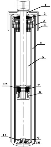
The internal structure of the shock absorber is relatively complex. The structure of a twin-tube hydraulic shock absorber is shown in Figure 1. Figure 1 indicates that the shock absorber is composed of a piston cylinder, a piston and a bottom valve. These parts divide the shock absorber into an upper chamber, a lower chamber and an oil storage chamber (Ju et al., 2014). The main damping components are the recovery valve and the flow valve on the piston. When the shock absorbers are in stretch operation, the recovery valve is used to relieve the vibration. When the shock absorbers are in compression operation, the flow valve mainly realizes the oil flow.

Figure 1. Structure of a twin-tube hydraulic shock absorber: 1, piston rod; 2, oil seal; 3, guide seat; 4, dust pad; 5, oil reservoir; 6, working cylinder; 7, recovery valve; 8, piston assembly; 9, compression valve; 10, bottom valve assembly; 11, compensation valve; 12, flow valve.

3. Fluid–solid coupling numerical method

Key technical difficulties in fluid–solid coupling involve not only the solution of the fluid model, but also the solution of the solid model (Jin, 2002). The fluid–solid coupling problem involves simultaneous solution and analysis of both fluid and solid, and is mainly used to solve the problem of the motion state between fluid and solid (Behera, 1992). Therefore, the basic principle of fluid–solid coupling needs to be studied from the aspects of both the fluid and the solid.

3.1. Fluid control equation

The flow of fluid needs to comply with the basic conservation law, which mainly consists of three parts: mass conservation law, energy conservation law and momentum conservation law (P. F. Liu, 2015).

3.1.1. Continuity equation

In the flow field, when the fluid flows into the control body from one control surface, it will also flow out of the control body from another control surface. In this process, the fluid quality in the control body will change (Wang, 2012). According to the mass conservation law in physics, the gap value between the inflow control body mass and outflow control body mass will be equivalent to the added mass of fluid inside the control body. According to the above theory, the fluid continuity integration equation is derived, as shown in formula (1): (1) $\frac{\mathrm{\partial }}{\mathrm{\partial }\text{t}}\underset{V}{\int \int \int }\rho \text{d}V\text{ + }\int \underset{S}{\int }\rho V\bullet \text{d}S=0$(1) where $\rho$ is the density of liquid, $V$ is the control volume, and $S$ is the control plane. In formula (1), the first term represents the growth rate of fluid mass in the control body, and the second term represents the net mass flow out of the entire control body through the control surface.

In Cartesian coordinates, formula (1) can be converted into a differential form, as shown in formula (2): (2) $\frac{\mathrm{\partial }\rho }{\mathrm{\partial }\text{t}}\text{ + }u\frac{\mathrm{\partial }(\rho u)}{\mathrm{\partial }x}+v\frac{\mathrm{\partial }(\rho v)}{\mathrm{\partial }y}+w\frac{\mathrm{\partial }(\rho w)}{\mathrm{\partial }z}=0$(2) where $u$ is the fluid speed component in the x direction, $v$ is the fluid speed component in the y direction, and $w$ is the fluid speed component in the z direction.

3.1.2. Momentum equation

In a given fluid system, the fluid momentum gradient over time is equivalent to all external forces acting on its surface (Li et al., 2010). This is the momentum conservation law of fluid in physics, and its differential expression is shown in formula (3): (3) $\{\begin{array}{l}\rho \frac{\text{d}u}{\text{d}t}=\rho F_{bx}+\frac{\mathrm{\partial }{p}_{xx}}{\mathrm{\partial }x}+\frac{\mathrm{\partial }{p}_{yx}}{\mathrm{\partial }y}+\frac{\mathrm{\partial }{p}_{zx}}{\mathrm{\partial }z}\\ \rho \frac{\text{d}v}{\text{d}t}=\rho F_{by}+\frac{\mathrm{\partial }{p}_{xy}}{\mathrm{\partial }x}+\frac{\mathrm{\partial }{p}_{yy}}{\mathrm{\partial }y}+\frac{\mathrm{\partial }{p}_{zy}}{\mathrm{\partial }z}\\ \rho \frac{\text{d}w}{\text{d}t}=\rho F_{bz}+\frac{\mathrm{\partial }{p}_{xz}}{\mathrm{\partial }x}+\frac{\mathrm{\partial }{p}_{yz}}{\mathrm{\partial }y}+\frac{\mathrm{\partial }{p}_{zz}}{\mathrm{\partial }z}\end{array}$(3) where $p_{xx}$, $p_{xy}$, $p_{xz}$, $p_{yy}$, $p_{yz}$ and $p_{zz}$ represent the components of the internal stress tensor of the fluid, and $F_{bx}$, $F_{\text{by}}$ and $F_{bz}$ respectively represent the mass force per unit fluid mass in the x, y and z directions.

3.1.3. Energy equation

According to the first law of thermodynamics (Tu & Zou, 2005), the energy equation of the fluid can be expressed by the relevant fluid physical quantity, as shown in formula (4): (4) $\begin{array}{rl}& \frac{\mathrm{\partial }}{\mathrm{\partial }\text{t}}(\rho E)+\frac{\mathrm{\partial }}{\mathrm{\partial }{x}_i}[u_i(\rho E+\rho )]\\ & =\frac{\mathrm{\partial }}{\mathrm{\partial }{x}_i}\left[k_{\text{eff}}\frac{\mathrm{\partial }T}{\mathrm{\partial }{x}_i}-\sum _{j^{\mathrm{\prime }}}{h}_{j^{\mathrm{\prime }}}{J}_{j^{\mathrm{\prime }}}+u_j{({\tau }_{ij})}_{\text{eff}}\right]+S_h\end{array}$(4) where $E=h-p/\rho +{u_i}^2/2$, $u_i$ is the velocity of fluid flow, $k_{\text{eff}}$ is the effective heat conduction coefficient, $k_{\text{eff}}=k+k_t$, $k_t$ is the turbulent heat conduction coefficient, $J_{j^{\mathrm{\prime }}}$ indicates component diffuse flux, and $S_h$ indicates the chemistry-generated heat and other customized definition volumetric heat sources. The first three distributions on the right-hand side of formula (4) describe the heat conduction, the diffuse component and the energy transport generated by sticky dissipation, respectively.

3.2. Solid control equation

Based on Newton’s second law, the conservation equation is obtained for the solid part, as shown in formula (5): (5) ${\rho }_s{\ddot{d}}_s=\mathrm{\nabla }\bullet {\sigma }_s+f_s$(5) where ${\rho }_s$ is the density of the solid, ${\sigma }_s$ is the Cauchy stress tensor, $f_s$ is the volume force vector, and ${\ddot{d}}_s$ is the regional acceleration vector.

3.3. Fluid–solid coupling solution equation

The fluid–solid coupling solution should follow the conservation law, and the fluid pressure is conserved or equal to the solid stress, the displacement, the heat flux, the temperature and other variables for the fluid–solid coupling interface (Y. Liu, 2015); that is, four basic equations are satisfied, as shown in formula (6): (6) $\{\begin{array}{l}{\tau }_f\bullet n_f={\tau }_s\bullet n_s\\ d_f=d_s\\ q_f=q_s\\ T_f=T_s\end{array}$(6) where ${\tau }_f$ and ${\tau }_s$ are fluid stress and solid stress, respectively; $n_f$ and $n_s$ are the boundary unit normal vectors of the fluid and solid, respectively; $d_f$ and $d_s$ are the displacements of fluid and solid after loading, respectively; $q_f$ is the heat flux through the fluid, $q_s$ is the heat flux through the solid; $T_f$ is the fluid temperature, and $T_s$ is the solid temperature.

4. Fluid–solid coupling modeling

4.1. Model simplification

Considering the huge amount of calculation required in the three-dimensional (3D) geometric model of the recovery valve of a vehicle shock absorber, to enhance the work efficiency of the recovery valve simulation analysis, while not deviating from the actual application, a 3D geometric model of the recovery valve is assumed and simplified.

1. The complete geometric model of the recovery valve of a vehicle shock absorber is highly complex, and there are many complicated auxiliary connecting parts, such as the adjusting valve piece, nut and spring leaf. The main areas of study are the velocity field, pressure field, temperature field, cavitation phenomenon and damping characteristics of the superposition valve slice. These components have little influence on the flow field near the superposition valve, so they can be ignored or simplified.

2. Because the through-hole of a vehicle shock absorber often exchanges oil, a reserved liquid clearance layer (He, Gu, & Long, 2012) with a height of 0.04 mm is inserted between the shock absorber piston and shock absorber superposition valve slice in the model, which is used to simulate the common through-hole flow rate and improve the calculation accuracy for the shock absorber.

3. Since the 1/4 3D geometric model of the recovery valve is consistent with the simulation results of the recovery valve overall model, to decrease the amount of calculation and increase the speed of calculation, the shock absorber oil reservoir and working cylinder are treated as rigid bodies, and the 1/4 model of the recovery valve is used for calculation in the simulation (Shams et al., 2007).

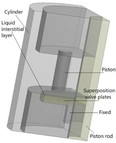
After simplification, according to the requirements of the parameter design mathematical model of the recovery valve, a 1/4 3D geometric model of the recovery valve of the vehicle shock absorber is drawn in PROE software. This model is shown in Figure 2.

Figure 2. A 1/4 three-dimensional geometric model of the recovery valve.

4.2. Establishment of shock absorber recovery valve fluid model

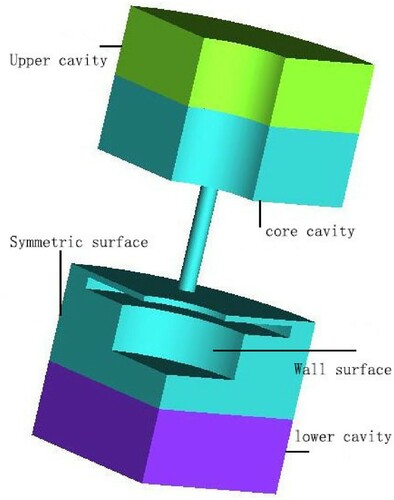
The established recovery valve 1/4 3D model is imported into Workbench software. The Fill operation is used to extract the recovery valve fluid model. A Boolean operation is used to trim the extracted recovery valve fluid model, and finally the recovery valve fluid model required for simulation is obtained. The recovery valve fluid model is shown in Figure 3. Figure 3 shows that the recovery valve fluid model is mainly composed of the upper oil cavity, lower oil cavity and core cavity (Wang et al., 2016).

Figure 3. Fluid model of the recovery valve.

4.3. Establishment of shock absorber recovery valve grid model

Jiang et al. (2012) studied the nonlinear characteristics of superposition of the shock absorber valve piece; however, they did not consider the reserved liquid gap layer, which is the ideal situation, and the recovery valve fluid grid adopted a tetrahedral mesh density. However, without considering the real operating conditions of a vehicle shock absorber, it is easy to make large computational errors.

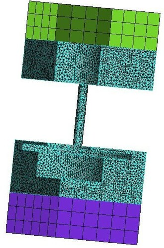
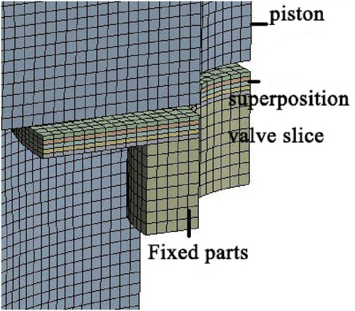
Based on the above analysis, the recovery valve fluid grid model is meshed, as shown in Figure 4. Figure 4 indicates that the flow fields of the key cavities change dramatically when the shock absorber is working normally. The key cavities of the shock absorber are divided into dense tetrahedral grids, with a total of 15,323 grids. The flow field varies smoothly in the upper oil cavity and the lower oil cavity. To decrease the work of calculation, the upper and lower oil cavities are meshed in sparse hexahedral grids, and the total number of grids is 3326. Considering the normal orifice oil flow, a reserved liquid gap layer is added between the piston and the superposition valve slice. All the variables of the recovery valve are established at the inflection point node, and the numerical calculation is accurate.

Figure 4. Grid model of the recovery valve.

4.4. Establishment of superposition valve slice model

The geometric model of the shock absorber recovery valve is imported into Workbench, and then the material properties and geometric properties of the recovery valve stack valve are defined in Workbench. The specific information is as follows: elastic modulus E = 1.8e5 MPa, density $\rho$ = 7800 kg/m³, Poisson’s ratio $\mu$ = 0.26, thickness h = 0.22 mm, inner radius a = 10 mm and outer radius b = 20 mm. The solid finite element model of the superposition valve slice is gained by meshing, as shown in Figure 5.

Figure 5. Solid finite element model of the superposition valve slice.

4.5. Setting of fluid–solid coupling surface

The recovery valve fluid grid model is mainly simulated in CFX. The solid model of the restoring valve superposition valve slice is mainly used for simulation calculations in ANSYS (Fang, 2012). Therefore, to connect the simulation data of the two calculations, the fluid–solid coupling surface must be set. Theoretically, superposition valve parts in contact with the oil fluid–solid interaction need to be set, but in general, only the superposition valve fluid–solid coupling surface is set on both sides.

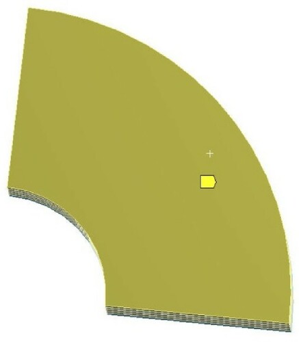
There are two main reasons for this. First, the outer edge of the superposition valve slices relative to the area of contact with the oil superposition valve slice surface is very small, and can be neglected. Second, when the superposition valve is open, there is deflection deformation, as shown in Figure 6. As can be seen from Figure 6, the nodes on the superposition valve slice are disturbed, which will lead to the parametric distortion of the fluid grid, affect the simulation results of fluid-solid coupling, and even make the simulation calculation difficult to carry out. Therefore, this paper only sets up two convection–solid coupling surfaces, on the upper and lower surfaces of the superimposed valve. The upper surface of the superposition valve slice fluid–solid coupling is shown in Figure 7, and the lower surface in Figure 8.

Figure 6. Schematic diagram of deflection deformation of the superposition valve slice.

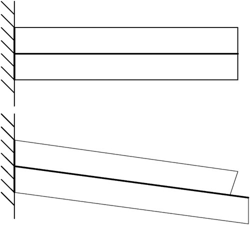
Figure 7. Superposition valve slice fluid–solid coupling: upper surface.

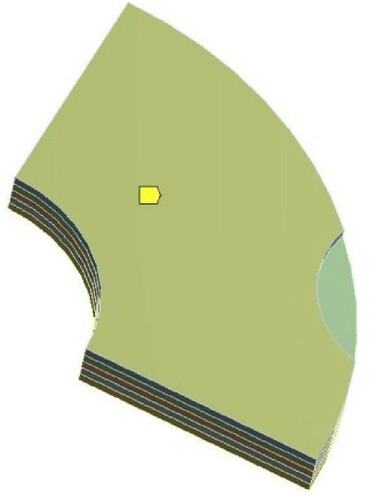
Figure 8. Superposition valve slice fluid–solid coupling: lower surface.

5. Analysis of simulation and test

5.1. Material setting of fluid–solid coupling

The simulation calculation of bidirectional fluid–solid coupling for a vehicle shock absorber is carried out in Workbench, for which the solid and fluid areas need to be set up. In the solid region, since the superposition valve slice has a preload that affects the analysis of the dynamic characteristics of the vehicle shock absorber, to reduce errors in the simulation calculation, the displacement load is set on the surface of the superposition valve slice to achieve the effect of simulation preload. To reach the goal of transferring solid and fluid information to each other, the upper and lower parts of the superposition valve slice are simultaneously regarded as fluid–solid coupling surfaces.

Since the inner radius of the superimposed disc hardly moves when opening the valve, the fixed load is set at the inner radius of the superimposed disc. For the fluid region, the shock absorber oil has a kinematic viscosity of 13.05 mm²/s, density of 870 kg/m³ and viscosity index of 198, and the reference pressure is set at 0 Pa. The fluid–solid coupling model is used for transient solution. The solution method is a standard model. This paper used a velocity-type fluid inlet and a pressure-type fluid outlet. In FLUENT, the superposition valve slice is set as system coupling to realize the simulation and calculation of the dynamic grid. The UDF (custom function) is used to achieve the purpose of interchanging the inlet velocity at any time with parabolic variations (Xin, 2013).

5.2. Solution setting of fluid–solid coupling

The simulation calculation solution is optimized and selected in Workbench software, to improve the effectiveness of the simulation and obtain better results.

1. To achieve better convergences and calculation accuracies, the relaxation factor has been set as 0.65.

2. The compressibility of the oil inside the shock absorber is ignored (Huang et al., 2013), and the friction between the shock absorber superposition valve slices and the friction between the piston rod and the guide seat are ignored (Yu et al., 2014).

3. Only the moving grid of superposition valve slices in the core area is considered.

4. Owing to the existence of large perturbation deformation in the superposition valve slice under stress, it was found that a penalty stiffness coefficient $F_{kn}\text{ = }1.0$ could solve the problem of large perturbation deformation of the superposition valve slice, so the penalty stiffness coefficient is set to $F_{kn}\text{ = }1.0$ (He, Long, & Xiao, 2012).

5. An adaptive step size is adopted and efforts are made to reduce the time step size to improve the computational efficiency under the condition of convergence.

5.3. Simulation analysis

The bidirectional fluid–solid coupling simulation diagram is shown in Figure 9. Under the effect of heterogeneity of oil pressure, the restoring valve stack valve plates of each area of the maximum stress and maximum deformation area are in different positions (Takahashi, 1996). The stress cloud chart of the superposition recovery valve slice is shown in Figure 10. The displacement cloud chart of the superposition recovery valve slice is shown in Figure 11.

Figure 9. Simulation block diagram of bidirectional fluid–solid coupling.

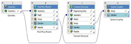
Figure 10. Stress cloud chart of the superposition recovery valve slice.

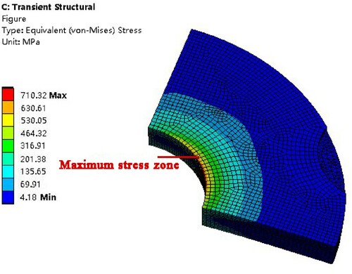
Figure 11. Displacement cloud chart of the superposition recovery valve slice.

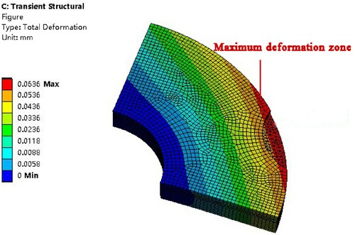
Figures 10 and 11 show that the maximum stress on the superposition valve slice occurs at the inner radius of the superposition valve slice, and the maximum stress is approximately 710.32 MPa. The maximum deformation area of the recovery valve superposition valve slice is near the piston hole, and the deformation of the recovery valve superposition valve slice is uniformly distributed, with the maximum deformation displacement being approximately 0.0636 mm. The greater the damping force, the greater the pressure fluctuation and the easier the deformation.

The recovery valve stack valve slice at a certain moment of internal displacement determines the instantaneous flow volume of shock absorber oil, and the oil flow size can influence the damping force for a vehicle shock absorber. Therefore, in the dynamic movement analysis of a vehicle shock absorber, recovery of the movement of the valve stack valve plate affects the size of the shock absorber damping force inside. The displacement–time diagram of the recovery valve superimposed plate is shown in Figure 12, and the speed–time diagram of the restoring valve stack plate is shown in Figure 13.

Figure 12. Displacement–time diagram of the recovery valve superimposed plate.

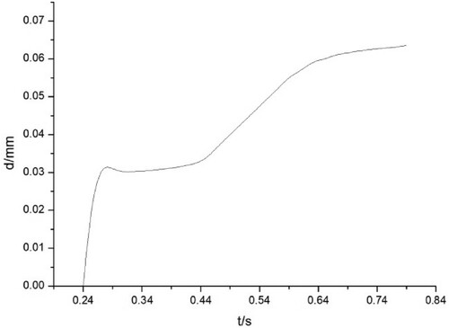
Figure 13. Speed–time diagram of the restoring valve stack plate.

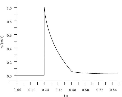
It can be seen from Figures 12 and 13 that the displacement value and velocity value of the maximum displacement point of the superposition valve slice recovery valve are both zero at the beginning of the operation of the vehicle shock absorber. When t is 0.24 s, the speed and displacement of the maximum displacement point of the recovery valve superposition disc suddenly increase, indicating that this is the opening time point of the shock absorber. As time goes on, the stress on the superposition valve slice increases gradually, and the displacement of the superposition valve slice also increases gradually. However, owing to the influence of the stiffness of the valve plate, the velocity of the maximum displacement point shows a nonlinear decrease. When the valve is completely opened, the velocity of the maximum displacement point of the superposition valve slice is 0, but the displacement reaches the maximum value. It can be seen from Figures 12 and 13 that the maximum displacement point of the superposition valve slice of the recovery valve and the time point of the abrupt change in velocity are almost the same, indicating that the fluid–solid coupling method has a good dynamic nonlinear analysis function and can accurately demonstrate the dynamic nonlinear response of the superposition valve slice of the vehicle shock absorber.

5.4. Test analysis

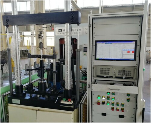
To verify the validity of the bidirectional fluid–solid coupling method proposed in this paper, a real shock absorber was used in an indicator test. The area, size and shape fullness of the indicator diagram obtained from the test can be used to judge the dynamic characteristics of the shock absorber to prove whether the simulation results are correct. Therefore, the combination of simulation analysis and experimental verification is a meaningful research method.

The shock absorber test platform is shown in Figure 14. The test equipment used in this study is the shock absorber servo dynamometer QJ-4A-10, and the dynamometer amplitude is 50 mm. The test environment is normal temperature. The accuracy and error have been analyzed and the relaxation factor is set as 0.65, which can obtain good convergence and simulation accuracy. In the experimental measurement stage, 20 double-cylinder hydraulic shock absorbers (model number S50-230 GH2), which have the same structural parameters, are regarded as the test samples. The test data adopt the average value and the mean square errors are calculated and analyzed to reduce the test error.

Figure 14. Shock absorber test platform.

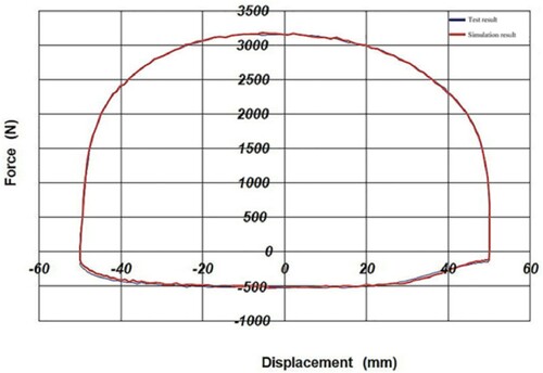
The shock absorber velocity characteristics chart is shown in Figure 15 and the shock absorber indicator characteristics chart is shown in Figure 16, which accurately demonstrates the indicator characteristics of the shock absorber. Figure 15 shows that the damping behavior of the shock absorber is asymmetric, and the force generated on extension of the shock absorber is three times larger than that on compression. Figure 16 shows that the damping behavior of the shock absorber is also asymmetric, and the force generated on extension of the shock absorber is six times larger than that on compression. It can be seen from Figures 15 and 16 that the simulation results of indicator performance are broadly in line with the test results, which indicates that the method proposed in this paper is accurate and dependable for simulating and analyzing the working conditions of the inside valve system of a shock absorber.

Figure 15. Shock absorber velocity characteristics chart.

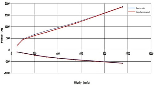
Figure 16. Shock absorber indicator characteristics chart.

The damping coefficient of a shock absorber is expressed by the equivalent dynamic damping coefficient, and the work done by the recovery stroke of the shock absorber is calculated by formula (7): (7) $\begin{array}{rl}W& =A_f={\int }_0^{\pi }{S}_1(t)dF(t)\\ & =\frac{\pi }{2}{C}_{f}w{S}_{max}^2\\ & ={\pi }^{2}f{C}_f{S}_{max}^2\end{array}$(7) where $S_1(t)=S_{\text{lmax}}\sin (wt)$ and $S_1(t)$ is the given simple harmonic excitation, $S_{\text{lmax}}$ is the excitation amplitude, w is vibration angular velocity, $A_f$ is the indicator characteristic chart area of the recovery stroke, $F(t)$ is the damping force of the recovery stroke, $S_{\text{max}}$ is the vibration amplitude of the piston, f is the excitation frequency, and $C_f$ is the damping coefficient of the recovery stroke.

According to formula (7) and Figure 16, the damping coefficient calculation in formula (8) can be obtained: (8) $C_f=\frac{A_f}{{\pi }^{2}f{S}_{max}^2}$(8) where $A_f$ = 0.211 $\text{kN}\cdot \text{m}$, f = 2.65 Hz and $S_{\text{max}}$ = 0.05 m, so the damping coefficient of the extension stroke shock absorber is 3.23 $\text{kN}\cdot \text{s}/\text{m}$.

This is similar to the calculation of the damping coefficient of the recovery stroke, and the damping coefficient of the compression stroke can be calculated by formula (9): (9) $C_y=\frac{A_y}{{\pi }^{2}f{S}_{max}^2}$(9) where $A_y$ is the area of the indicator characteristics chart of the compression stroke, and $A_y$ = 0.040 $\text{kN}\cdot \text{m}$, so the calculated damping coefficient of the compression stroke is 0.615 $\text{kN}\cdot \text{s}/\text{m}$. The damping coefficient of the recovery stroke is about 5.25 times greater than the damping coefficient of the compression stroke for the shock absorber. The damping force of the shock absorber is related to the damping coefficient. The greater the damping coefficient, the greater the damping force. Therefore, it can be seen from Figure 16 that the damping force of the recovery stroke is much greater than the damping force of the compression stroke, and the damping force of the recovery stroke is about six times the damping force of the compression stroke.

The impact force of the vehicle is absorbed mainly through the shock absorber’s compression stroke, and the shock absorber converts kinetic energy into elastic potential energy. When the compression damping force is small, the shock absorber can absorb the impact effectively. The energy absorbed by the shock absorber is released in the form of heat energy through the recovery stroke. The bigger the damping force in the recovery stroke, the more energy is released by the shock absorber. There will be less energy transferred to the vehicle and passengers will be more comfortable. Research results show that when the restored damping force is large, the vibration of the car body rapidly decreases and better ride comfort can be obtained.

6. Conclusions and future work

This paper has established and analyzed the fluid control equation, solid control equation and fluid–solid coupling solution equation, and the damping coefficient of the shock absorber has been calculated and selected. On the strength of the fluid–solid coupling method, a high-precision flow grid model and a solid finite element model of the stacked valve are built and analyzed. A bidirectional fluid–solid coupling method is proposed in this paper, which can be adopted to simulate and analyze the dynamic nonlinear response characteristics of a stacked valve slice of a vehicle shock absorber in Workbench software. The study results indicate that the superposition valve slice maximum occurs at the inner radius, but the maximum deformation area is near the piston hole, and the maximum deformation is about 0.0636 mm. When the stack valve plate just opens the valve, the displacement and speed of the stack valve plate will simultaneously produce a jump change. The results of the calculation analysis are broadly in line with the test results, which indicates that the method proposed in this paper is accurate and dependable.

The research demonstrates that this method can reduce the dependence on experiments in the development process of vehicle shock absorbers, and improve the design precision of the superposition of vehicle shock absorber valve plates. In summary, the method proposed in this paper can be used effectively to enhance the quality of vehicle shock absorbers and shorten the development cycle, which has important theoretical and practical value. In the future, the authors plan to research the compression valve internal situation and the cavitation for vehicle shock absorbers, to further improve the quality of vehicle shock absorbers.

Acknowledgements

The authors would like to thank the anonymous reviewers for their helpful comments and suggestions for improving the manuscript.

Disclosure statement

No potential conflict of interest was reported by the authors.

Additional information

Funding

This research was supported by the Key Research Program of Jiangxi Province [grant number 20171BBE50039] and the National Natural Science Foundation of China [grant number 51565011].

References

- Behera, N. (1992). On the solutions of fluid flow and solid deformation interaction problems. The Ohio State University.
- Chen, Q. P., Shu, H. Y., & Fang, W. Q. (2013). Fluid structure interaction for circulation valve of hydraulic shock absorber. Journal of Central South University, 20(3), 648–654. https://doi.org/https://doi.org/10.1007/s11771-013-1531-x
- Czop, P., Gasiorek, D., & Gnilka, J. (2012). The fluid-structure simulation of a valve system, informs in hydraulic dampers. Modelowanie Inżynierskie, 14(45 s 197), 205.
- Duan, F. B., Pan, J., & Chen, W. H. (2017a). Damping force modeling and sensitivity analysis of double-tube hydraulic damper. Chinese Journal of Engineering Design, 24(2), 149–155. https://doi.org/https://doi.org/10.3785/j.issn.1006-754X.2017.02.004
- Duan, F. B., Pan, J., & Chen, W. H. (2017b). Modeling and reliability evaluation of damping force degradation of double-cylinder hydraulic shock absorber. Chinese Journal of Mechanical Engineering, 53(24), 201–210. https://doi.org/https://doi.org/10.3901/JME.2017.24.201
- Fang, W,Q. (2012). Finite element reconstruction calculation and analysis of the dynamic characteristics of automobile hydraulic shock absorber valve plate. Chongqing University.
- Ghalandari, M., Bornassi, S., & Shamshirband, S. (2019). Investigation of submerged structures’ flexibility on sloshing frequency using a boundary element method and finite element analysis. Engineering Applications of Computational Fluid Mechanics, 13(1), 519–528. https://doi.org/https://doi.org/10.1080/19942060.2019.1619197
- Guntur, H. L., & Hendrowati, W. (2015). A Comparative study of the damping force and energy absorbtion capacity of regenerative and conventional-viscous shock absorber of vehicle suspension. Applied Mechanics and Materials, 758, 45–50. https://doi.org/https://doi.org/10.4028/www.scientific.net/AMM.758.45
- He, L. P., Gu, L., & Long, K. (2012). Simulation analysis of dynamic characteristics of automotive shock absorbers based on fluid solid coupling. Journal of Mechanical Engineering, 48(13), 96–101. https://doi.org/https://doi.org/10.3901/JME.2012.13.096
- He, L. P., Long, K., & Xiao, J. P. (2012). Finite element analysis of ANSYS 13.0 and HyperMesh 1.0 Co-simulation [M]. Machinery Industry Press.
- Huang, X. X., Yang, Y., & Shen, Y. Y. (2013). Characteristics analysis of hydro pneumatic suspension based on gas dissolution and oil compressibility. Transactions of the Chinese Society for Agricultural Machinery, 44(6), 14–18. https://doi.org/https://doi.org/10.6041/j.issn.1000-1298.2013.06.003
- Jiang, H. C., Zhang, N., & Yu, Z. H. (2012). Nonlinear characteristics simulation analysis of shock absorber throttle valves. Computer Simulation, 29(5), 338–342. https://doi.org/https://doi.org/10.3969/j.issn.1006-9348.2012.05.083
- Jin, Y. (2002). Numerical study on fluid solid coupling in turbine-turbine-Induced vibration of some airflow. Tsinghua University.
- Ju, R., Liao, C. R., & Zhou, Z. J. (2014). Car mr fluid shock absorber with mono-tube and charged-gas bag. Journal of Vibration and Shock, 33(19), 86–92. https://doi.org/https://doi.org/10.13465/j.cnki.jvs.2014.19.015
- Li, X. B., Shen, J. S., & Ning, X. B. (2010). Restriction characteristic study of shock absorber superimposition restoration valve based on fsi. Jiangsu Machine Building & Automation, 39(4), 20–22. https://doi.org/https://doi.org/10.3969/j.issn.1671-5276.2010.04.007
- Liu, P. F. (2015). Thermal load analysis of key components in the improvement of high-power special diesel engine.
- Liu, Y. (2015). Study on fluid solid coupling of axial flow suspended tidal current turbine. Zhejiang Ocean University.
- Lv, Z. H., Wu, Z. A., & Li, S. M. (2003). Finite element simulation of nonlinear dynamic characteristics of hydraulic damper's valve. Journal of Mechanical Strength, 25(6), 614–620. https://doi.org/https://doi.org/10.3321/j.issn:1001-9669.2003.06.005
- Salih, S. Q., Suliman, M., & Rasani, M. R. (2019). Thin and sharp edges bodies-fluid interaction simulation using cut-cell immersed boundary method. Engineering Applications of Computational Fluid Mechanics, 13(1), 860–877. https://doi.org/https://doi.org/10.1080/19942060.2019.1652209
- Shams, M., Ebrahimi, R., & Raoufi, A. (2007). CFD-FEA analysis of hydraulic shock absorber valve behavior. International Journal of Automotive Technology, 8(5), 615–622.
- Takahashi, K. (1996). Force extracting device for dampers: U.S. Patent 5, 507, 371 [P].
- Tu, W. G., & Zou, Y. S. (2005). Semi-active control of buildings based on energy response. Earthquake Engineering and Engineering Vibration, 25(3), 145–151. https://doi.org/https://doi.org/10.3969/j.issn.1000-1301.2005.03.025
- Wang, Q. L. (2012). Performance analysis and flow field simulation study of vertical grinding powder based on multiphase flow technology. University of Jinan.
- Wang, R., Gu, F., & Cattley, R. (2016). Modelling, testing and analysis of a regenerative shock absorber system. Energies, 9(5), 386–409. https://doi.org/https://doi.org/10.3390/en9050386.
- Xin, Y. (2013). Application research of fluent UDF method in numerical wave flume. Dalian University of Technology.
- Yang, P. (2001). An experimental study for the characteristics of a solid-fluid coupling shock absorber. Journal of Experimental Mechanics, 16(2), 226–231. https://doi.org/https://doi.org/10.3969/j.issn.1001-4888.2001.02.015
- Yu, Z. H., Liu, S. N., & Zhang, N. (2014). Multi-field coupling simulation analysis of mr damper. Transactions of the Chinese Society for Agricultural Machinery, 45(1), 1–7. https://doi.org/https://doi.org/10.6041/j.issn.1000-1298.2014.01.001
- Zhou, C. C., Pan, L. J., & Yu, Y. W. (2016). Optimal damping matching for shock absorber of vehicle leaf spring suspension system. Transactions of the Chinese Society of Agricultural Engineering, 32(7), 106–113. https://doi.org/https://doi.org/10.11975/j.issn.1002-6819.2016.07.015