Flow control using fluidic oscillators on an airfoil with a flap

Abstract

This study numerically evaluates the performance of flow control using fluidic oscillators on the NACA 0015 airfoil with a flap at different flap angles and different pitch angles of the oscillators. An inline array of fluidic oscillators is located just in front of the flap. Aerodynamic analysis was carried out using three-dimensional unsteady Reynolds-averaged Navier-Stokes equations in a computational domain that consists of the external domain around the airfoil and the internal domains in three fluidic oscillators. Flap angles of 20°, 40°, and 60° were tested with a fixed angle of attack of 8°. For each flap angle, the effects of the pitch angle of the oscillators on the aerodynamic performance were evaluated in a range of 60° to the negative value of the corresponding flap angle. It was found in this work that the oscillator jets parallel to the flap showed the best performance, which was achieved by using negative pitch angles and also bending the outlets of the oscillators. The results indicate that the aerodynamic performance varies significantly with the flap and pitch angles.

KEYWORDS:

• Fluidic oscillators
• flow separation control
• airfoil
• flap
• pitch angle
• Reynolds-averaged Navier-Stokes equations

NOMENCLATURE

Anozzle	=	Nozzle area of fluidic oscillator
CL	=	Lift coefficient
CD	=	Drag coefficient
Cp	=	Pressure coefficient
Cμ	=	Momentum coefficient
c	=	Chord length
s	=	Span length
h	=	Fluidic oscillator height
n	=	Number of fluidic oscillators
l	=	Length between fluidic oscillators
$\dot{m}$	=	Mass flow
L	=	Lift force
D	=	Drag force
Ps	=	Static pressure
Ps,∞	=	Free-stream static pressure
q∞	=	Free-stream dynamic pressure
T	=	Time
U	=	Velocity
U∞	=	Free-stream velocity
Ujet	=	Jet velocity at throttle nozzle of fluidic oscillator
Ux	=	Streamwise velocity
$\overline{U_x}$	=	Time averaged streamwise velocity
w	=	Fluidic oscillator width
wc	=	Inlet chamber width
wi	=	Inlet nozzle width
wt	=	Outlet throttle
x, y, z	=	Cartesian coordinates
x0	=	Location of fluidic oscillator
α	=	Angle of attack
β	=	Pitch angle
δf	=	Flap angle
θdiff	=	Diffuser angle of outlet nozzle
ρ∞	=	Density of working fluid at the external domain
ρjet	=	Density of working fluid at fluidic oscillator
ωy	=	Streamwise vorticity
$\overline{{\omega }_y}$	=	Time-averaged streamwise vorticity

1. Introduction

A variety of techniques have been introduced for flow control to delay or prevent flow separation on airfoils (Cully et al., 2004; Jhonston & Nishi, 1990; Lin et al., 1994). Active flow control (AFC) makes up for disadvantages of passive control and improves the control performance (Joshi & Gujarathi, 2016; Rivir et al., 2000). Among AFC devices, a fluidic oscillator converts steady-state inlet flow into vibrating outlet flow without any driving component, which energizes the boundary-layer flow on an airfoil to delay flow separation. Flow oscillators have been studied widely for their design simplicity and effective flow control performance (Jones et al., 2017; Kim & Kim, 2020; Koklu & Owens, 2014).

Koklu and Owens (2014) compared experimentally different techniques of flow control. Fluidic oscillators exhibited the best control performance among them in reducing flow separation. Jones et al. (2017) compared and analyzed the performance of flow separation control using steady-jets and fluidic oscillators at a Reynolds number of an actual flight. The fluidic oscillators had a mass flow rate that was 54% less than that of the steady-jet actuators and showed similar performance.

In recognition of the excellent performance of fluidic oscillators, various studies are being conducted for commercialization. Jeong and Kim (2018) carried out parametric studies and multi-objective optimization of fluidic oscillators to simultaneously improve maximum speed and pressure drop at the outlet of fluidic oscillators, which are affected by the splitter distance and the nozzle width at the inlet. Pandey and Kim (2018a, 2018b) performed analyses using Reynolds-averaged Navier-Stokes (RANS) equations and large eddy simulation for fluidic oscillators.

Melton et al. (2016) optimized the internal shape of fluidic oscillators and evaluated their aerodynamic performance by attaching them to a NACA 0015 airfoil. The aerodynamic performance was affected considerably by the change in the internal geometry of the oscillators. Melton and Koklu (2016) tested different sizes of fluidic oscillators installed in front of flap on an airfoil. Larger sizes exhibited better flow control in a wind tunnel experiment. There were also investigations on numerical analysis of external flows to improve accuracy of prediction (Ghalandari et al., 2019; Salih et al., 2019).

The flow separation control is affected by many geometric and operating parameters of fluidic oscillators. On an airfoil, the mounting conditions of fluidic oscillators, such as the location, angle, and arrangement, are also important for flow control. Koklu (2018) tested two locations of oscillators on a ramp model, experimentally. As the oscillators move closer to the flow separation, the pressure recovery became higher. Kim and Kim (2019) studied on the oscillators’ installation conditions (position, arrangement, and angle) on a humped surface. The control performance was best when the oscillators were arranged in a row and mounted immediately behind the flow separation. The performance was more sensitive to the pitch angle of the oscillators than their roll and yaw angles.

Kim and Kim (2020) studied on the oscillator location on an airfoil without a flap for different attack angles. The mounting location that was most effective in increasing the lift was affected by the angle of attack. However, the drag decreased as the location of the fluidic oscillators moved upstream for all the tested angles of attack. Woszidlo (2011) carried out an experiment to estimate the aerodynamic performance of oscillators according to the length and angle of the flap on an airfoil. They reported that, as the flap length and angle increased, the flow rate of the oscillators to control the flow separation increased.

Many studies have been performed on flow separation control according to the mounting conditions of fluidic oscillators. It was confirmed that the pitch angle of fluidic oscillators has a sensitive effect on the flow control. The performance of the fluidic oscillators mounted upstream of the flap is expected to be affected by the flap angle. A previous study extensively analyzed the influence of the mounting conditions on the aerodynamic performance in the case without flap (Kim & Kim, 2020). However, the relationship between the flap angle of an airfoil and mounting conditions of fluidic oscillators has not been studied previously.

The present numerical study examined the pitch angle of fluidic oscillators to find its effect on the flow separation for different flap angles of an airfoil (NACA 0015). The fluidic oscillators were installed just in front of the flap. For some pitch angles closer to the flap angle, fluidic oscillators with bent outlets were applied to overcome the geometrical limitations of inserting the oscillators into the airfoil. The flow inside the oscillators and external flow over the oscillating jets were analyzed using unsteady RANS equations. The major challenge in this work was to make the jets from the oscillators nearly parallel to the flap surface, which was achieved by adjusting the pitch angle of the oscillators and also bending the outlet parts of the oscillators.

2. Fluidic oscillator model and computational domain

Flow separation control was studied using fluidic oscillators, as shown in Figure 1. The oscillators were mounted on an airfoil (NACA 0015) with a flap. The oscillator used in this study has feedback channels and was first proposed by Stouffer (1979). As shown in Figure 1(b), the oscillator model was optimized by Melton et al. (2016). Table 1 shows a summary of the geometrical parameters.

Figure 1. Flow configuration and fluidic oscillator model: (a) airfoil model with fluidic oscillators and (b) fluidic oscillator model.

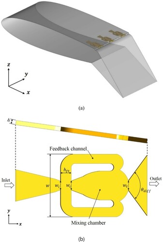
Table 1. Parameters of the tested fluidic oscillator.

Parameter	Value
Fluidic oscillator width, w (mm)	14.306
Inlet nozzle width, wi (mm)	2
Inlet chamber width, wc (mm)	2.03
Outlet throttle width, wt (mm)	2
Fluidic oscillator height, h (mm)	1
Inlet nozzle feedback channel width, $h_{ft}$ (mm)	2.41
Diffuser angle of outlet nozzle, θdiff (°)	107

The oscillator emits an oscillating jet, but there is no driving device inside the oscillator. A steady flow proceeds through the inlet of the oscillator to the main chamber, and flows along a side wall of the chamber as a result of the Coanda effect (Panitz & Wasan, 1972). Approaching the chamber exit, a part of flow goes back to the inlet of the oscillator using the feedback channels and a vortex is produced upstream of the chamber. The vortex with increased strength moves the main stream to the different chamber side. This process causes oscillating jets at the exit. Fluidic oscillators can be applied in various ways, and many studies are being conducted for their application to flow control (Raman & Raghu, 2004). Recently, research has also been actively conducted in the field of heat transfer (Kim et al., 2019), including film cooling (Hossain et al., 2019).

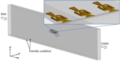
The computational domain is composed of the oscillator internal domains and the external domain of the airfoil, as shown in Figure 2. Periodic conditions were used to set up the computational domain to include 3 oscillators. To determine the number of oscillators included in the domain, 2, 3, and 4 oscillators were analyzed and compared in a preliminary study, as shown in Table 2. There is only a slight difference in the predicted lift and drag coefficients between 3 and 4 oscillators. Based on the results for the computational time and lift and drag coefficients, the case with 3 oscillators was judged to be most suitable.

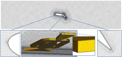
Figure 2. Computational domain.

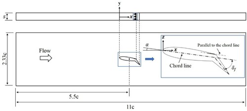
Table 2. Comparison of lift coefficients, drag coefficients and computational times for different numbers of fluidic oscillators (x₀/c = 0.7, α = 8°, δ_f = 40°, C_μ= 2.34%).

Number of fluidic oscillators	Exp. Melton et al. (2018)	2	3	4
Lift coefficient	2.33	2.070	2.145	2.144
Drag coefficient	–	0.147	0.161	0.165
Computational time (hours)	–	36	49	62
Relative error of lift coefficient (%) compared with experimental result	–	12.56	8.62	8.67

For the external domain, the experiment of Melton (2014) was referenced. The experiment was performed for various mass flows and flap angles of a flap located at 30% chord from the trailing edge. As shown in Figure 1(a), the oscillators were mounted in front of the flap. Melton et al. (2018) evaluated the aerodynamic performance of oscillators and steady jets according to the flow rate for various flap angles and angles of attack of the NACA 0015 airfoil. The angle of attack (α) was 8°, the range of the flap angle (δ_f) was 0° – 60°. At δ_f = 0°, the chord (c) and the span were 305 and 99 mm, respectively. The oscillators are mounted parallel to the chord line in front of the flap. In the present work, these experimental conditions were used as reference conditions for the testes of grid-dependency and validation.

The effect of the mounting pitch angle (β) of the oscillators on the flow control was investigated. The pitch angle was defined by the angle between the center line of the exit nozzle of an oscillator and the chord line of the airfoil, as shown in Figure 3. For each flap angle of 20°, 40°, and 60°, the tested range of the pitch angle was 60° ≥ β ≥ -δ_f. Plane A-A’ rotates around point A according to the pitch angle, and the oscillator exit plane is always perpendicular to this plane.

Figure 3. Installation conditions of fluidic oscillator.

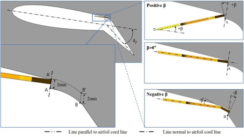
In the positive pitch-angle range, the orientation of the oscillators changes according to the pitch angle; i.e. plane A-A’ rotates around point A according to the pitch angle. However, in the negative pitch-angle range, the outlet nozzles of the oscillators are bent at the throat due to geometrical limitations, and the main body of the oscillators is fixed in the direction of zero pitch angle, as shown in Figure 3. Thus, the main bodies of the oscillators are parallel to the chord line of the airfoil for β ≤ 0, but their orientation changes according to β for the positive β range, as shown in Figure 3.

For all the flap angles, it is not possible to inject the jet parallel to the flap surface from plane A-A’. Therefore, for negative pitch angles, the location of the oscillator exit is moved downstream from plane A-A’ to plane B-B’, which rotates around point B according to the pitch angle. The distances between A and B are 3, 7, and 10.3 mm for δ_f = 20°, 40° and 60°, respectively. The location of the nozzle exit varies slightly on B-B’ depending on the pitch angle due to the geometry.

3. Performance parameters

The lift (C_L), drag (C_D), and pressure (C_P) coefficients are defined as follows: (1) $\begin{array}{rl}{C}_L& =\frac{L}{\frac{1}{2}{\rho }_{\mathrm{\infty }}{U}_{\mathrm{\infty }}^{2}cs}\end{array}$(1) (2) $\begin{array}{rl}{C}_D& =\frac{D}{\frac{1}{2}{\rho }_{\mathrm{\infty }}{U}_{\mathrm{\infty }}^{2}cs}\end{array}$(2) (3) $\begin{array}{rl}{C}_P& =\frac{P_s-P_{s,\mathrm{\infty }}}{\frac{1}{2}{\rho }_{\mathrm{\infty }}{U}_{\mathrm{\infty }}^2}\end{array}$(3) where L, D, P, ρ, U, c, and s indicate the lift force, drag force, pressure, fluid density, velocity, airfoil cord length, and width of the computational domain, respectively. The subscripts s and ∞ indicate static pressure and free-stream values, respectively.

4. Numerical analysis

Unsteady flow analysis of the internal flow of the oscillators and external flow on the airfoil was performed using the software ANSYS CFX 15.0® (ANSYS, 2014). The three-dimensional unsteady RANS equations and the continuity equation were used for the analysis along with the shear stress transport (SST) turbulence model. The SST model is known to accurately predict flow separations in adverse pressure gradients (Bardina et al., 1997; Menter, 1994).

Figure 4 shows the conditions applied at the boundaries of the computational domain with three oscillators. At the inlet, a uniform velocity of 25 m/s was applied, which was calculated from Reynolds number of 5.0×10⁵ using the chord length and inlet velocity. At the outlet, a constant pressure condition was used. At the walls, no-slip conditions were used. Periodic conditions were employed considering periodicity. The air was assumed to be an ideal gas at 25°C.

Figure 4. Computational domain using periodic boundary conditions.

Melton et al. (2018) performed an experiment for separation control by changing the momentum coefficient C_μ in the range of 0–6.63% for various flap angles. In this experiment, as the angle of flap and C_μ increased, the lift coefficient tended to increase. As the angle of flap increased, the flow separation area became larger, and larger C_μ was required. Thus, based on these experimental results, the C_μ value that had the best separation control performance for each flap angle was used, as shown in Table 3.

Table 3. Values of momentum coefficient for different flap angles.

Flap angle (°)	Cμ (%)
20	0.89
40	2.65
60	4.58

C_μ is defined as follows: (4) $C_{\mu }=\frac{n{\rho }_{jet}{U}_{jet}{A}_{nozzle}{U}_{jet}}{\frac{1}{2}{\rho }_{\mathrm{\infty }}{U}_{\mathrm{\infty }}^{2}cnl}=2\frac{A_{nozzle}}{cl}{\left(\frac{U_{jet}}{U_{\mathrm{\infty }}}\right)}^2$(4) where (5) $U_{jet}=\frac{\dot{m}}{{\rho }_{jet}{A}_{nozzle}}=\frac{\dot{m}}{{\rho }_{\mathrm{\infty }}{A}_{nozzle}}$(5) where U_jet is the exit velocity of the oscillators, A_nozzle is the area of the oscillator nozzle outlet, $\dot{m}$ (= ρ_jet U_jet A_nozzle) is the mass flow rate, n is the number of oscillators, and l is the spacing between the oscillators. The wing length s was the same as the product of the number of oscillators and the spacing. ρ_jet is the fluid density of the jets, which is equal to the density of the external flow, ρ_∞. With this assumption, U_jet is determined by Equation (5).

Figure 5 shows the grid system used. A prism mesh was constructed in near-wall region, and the other areas had an unstructured tetrahedral mesh. To use the SST model developed for low Reynolds numbers, the grid points nearest from the wall were placed in y⁺ < 2.

Figure 5. Grid system (α = 8° and δ_f = 40°).

As the convergence criterion, the root-mean-square residuals were kept smaller than 1.0×10⁻⁴. The total time was 0.03 s per case, and the time step was selected as 5×10⁻⁶s. The steady RANS analysis results were used as the initial guess for the unsteady analysis. The simulation was carried out using a Super Computer which uses an Intel Xeon Gold 6148/2.4GHz processor with 32 CPU cores. It took about 48 h to calculate a single case.

5. Results and discussion

5.1. Analysis of grid convergence index

Grid-convergence index (GCI) analysis was carried out using Richardson extrapolation (Celik et al., 2008; Roache, 1998) to evaluate the convergence of grid system, as shown in Table 4, for the internal domain of an oscillator. The relative discretization error $\left(GC{I}_{fine}^{21}\right)$ was 0.957%, so the finest grid system with 4.7 × 10⁵ cells in an oscillator was selected for further calculations. Table 5 presents the analysis results for lift coefficient C_L for the external domain. The grid system with 2.2×10⁶ cells was confirmed to converge for the external domain. Therefore, a total of 3.8×10⁶ grid nodes was used in the whole computational domain for further calculations.

Table 4. Grid convergence index (GCI) analysis for the internal domain of a fluidic oscillator.

Parameter		Value
Number of cells	N1 / N2 / N3	4.7×10^5 / 3×10^5 / 2.1×10^5
Grid refinement factor	r	1.3
Computed jet frequencies corresponding to N1, N2, and N3	f1	1176.5
	f2	1272.4
	f3	1176.5
Apparent order	p	4.93
Extrapolated values	${\varphi }_{ext}^{21}$	1308.6
Approximate relative error	$e_a^{21}$	2.025%
Extrapolated relative error	$e_{ext}^{21}$	0.759%
Grid convergence index	$GC{I}_{fine}^{21}$	0.957%

Table 5. Grid convergence index (GCI) analysis for the external domain of airfoil.

Parameter		Value
Number of cells	N1 / N2 / N3	2.2×10^6 / 1.6×10^6 / 1.1×10^6
Grid refinement factor	r	1.3
Computed lift coefficients (C L) corresponding to N1, N2, and N3	CL1	2.135
	CL2	2.147
	CL3	2.198
Apparent order	p	5.51
Extrapolated values	${\varphi }_{ext}^{21}$	2.131
Approximate relative error	$e_a^{21}$	0.562%
Extrapolated relative error	$e_{ext}^{21}$	0.188%
Grid convergence index	$GC{I}_{fine}^{21}$	0.072%

5.2. Validation of numerical results

Using experimental data obtained by Melton et al. (2018), the computational results for both the external and internal flow domains were validated. The numerical results for the flow in a single oscillator were validated for the jet frequency in Table 6. The results show that the difference between the experimental measurement and numerical result for the frequency decreases as C_μ (or the flow rate) increases.

Table 6. Validation of numerical results for jet frequency of fluidic oscillators.

	Jet frequency, Hz
Cμ, %	CFD	Exp.	Relative error, %
0.89%	734	810	10.31
2.65%	1052	1130	7.35
4.58%	1197	1300	8.58
6.63%	1300	1350	3.85

Validation of the results in the external flow domain was also performed for both the pressure and lift coefficient distributions of the airfoil, as shown in Figures 6 and 7. The validation for the lift coefficient of the airfoil with a flap was performed at C_μ = 2.15% and δ_f = 40°. Figure 6 shows a comparison between the experimental data and numerical results for the variation of the lift coefficient at different angles of attack. As the angle of attack increases, the error decreases, and the two results become almost identical at 11° before stall occurs. It seems that several factors including flap angle, oscillator location and flow rate, are concerned to the errors. Further study is needed to clarify the reason for the errors. The analysis in this work was performed at an angle of attack of 8°. Woszidlo’s (2011) numerically predicted lift coefficient was about 50% than the experimental data for α = 0° and δ_f = 30° for a 36% chord trailing edge flap.

Figure 6. Comparison between numerical results and experimental data for lift coefficient (Melton et al., 2018) for the airfoil with fluidic oscillators (x₀/c = 0.7, α = 8°, δ_f = 40°, C_μ= 2.15%).

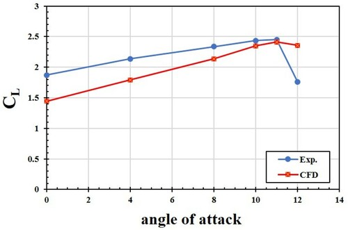
Figure 7. Comparison between numerical results and experimental data for pressure coefficient (Melton et al., 2018) for the airfoil with fluidic oscillators (x₀/c = 0.7, α = 8°, δ_f = 40° and y/s = 0.5).

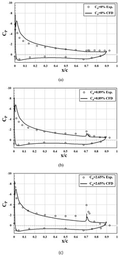
Validation of the pressure coefficient distributions on the airfoil was carried out at a flap angle δ_f = 40° with three different mass flow conditions of the oscillators (C_μ= 0%, 0.89%, and 2.65%), as shown in Figure 7. The results agree well on the lower side of the airfoil regardless of mass flow. However, on the upper side, some discrepancies were found near the leading edge at the two lower C_P values and near the trailing edge at the highest C_P.

5.3. Aerodynamic performance

5.3.1. Lift coefficient

The results of predictions for the lift coefficient of the airfoil depending on the pitch angle of the oscillators at three flap angles are shown in Figure 8. The C_μ value that showed the best pressure recovery for each flap angle (Melton, 2014) was used in this calculation. Figures 8(a and b) show the lift coefficient (C_L) and relative lift increment (ΔC_L/C_L,base) variations with the pitch angle, respectively. Lift increment (ΔC_L) is the increase in the lift coefficient compared with the case without oscillators (C_L,base), which indicates the quantitative effect on the lift coefficient.

Figure 8. Variations of lift coefficient and its relative increment with pitch angle of fluidic oscillators for different flap angles: (a) lift coefficient and (b) normalized lift increment.

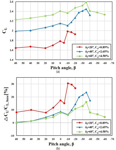
The lift coefficient generally increases as the pitch angle decreases and reaches a maximum value at a pitch angle close to the negative value of the flap angle, as shown in Figure 8(a). This indicates that up to a certain pitch angle, the lift coefficient increases as the jet injection from the oscillators becomes more parallel to the flap. But a small decrease in the lift coefficient is commonly found at the first negative pitch angles. These drops in lift coefficient seem to be caused by the change in the installation location (from A to B in Figure 3) for negative pitch angles. Thus, they are not regarded as a pure effect of the pitch-angle change. It is interesting that the pitch angle where the maximum C_L occurs for C_μ= 2.65 (β = −35°) is the same as that for C_μ= 4.58, and the trends of the C_L variation are also similar for these two C_μ values. In contrast, if the pitch angle has positive values, the lift coefficient becomes less than that at the reference condition (β = 0°).

In Figure 8(b), the relative lift increment for the flap angle δ_f = 20° shows remarkably larger values than those for δ_f = 40° and 60° in the whole range of pitch angle. The highest maximum relative lift increment of about 30% was obtained at β = −10° for δ_f = 20°. In the cases of flap angles of 40° and 60°, the variations of the relative lift increment with β are nearly the same in the range of 60° ≥ β ≥ −10°, but the maximum relative lift increment for δ_f = 40° is much larger than that for δ_f = 60° at β = −35°.

5.3.2. Drag coefficient

The variations of the drag coefficient (C_D) and relative drag decrement (ΔC_D/C_D,base) with pitch the angle for three flap angles are shown in Figure 9(a) and (b). The drag decrement (ΔC_D) indicates the decrease in drag coefficient compared to the drag coefficient without oscillators (C_D,base). Figure 9(a) shows that the drag coefficient has less variation than the lift coefficient. As the flap angle increases, the variation of the drag coefficient becomes larger. The drag coefficient is nearly uniform for δ_f = 20°, but it decreases as the pitch angle decreases for δ_f = 40°. In the case of δ_f = 60°, the maximum C_D was found in the range of 0° ≥ β ≥ −20°. This means that in this case of high flap angle, even a positive pitch angle reduces the drag compared to the reference condition (β = 0°). The reason for the sudden increase in C_D at β = 0° for δ_f = 60° is not clear, and further study is needed to clarify it.

Figure 9. Variations of drag coefficient and its relative decrement with pitch angle of fluidic oscillators for different flap angles: (a) drag coefficient and (b) normalized drag decrement.

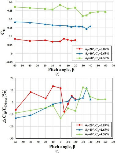
For the two higher flap angles, δ_f = 40° and 60°, negative pitch angles reduce the drag coefficient less than at the reference condition (Figure 9(a)) and also improve the lift coefficient (Figure 8(a)). At a flap angle of δ_f = 20°, a rise in the drag coefficient and a drop in the lift coefficient occurs at β = −5°. For flap angles of δ_f = 40° and 60°, the maximum C_L and minimum C_D were found at β = −30° or −35°.

As shown in Figure 9(b), the drag reduction due to the oscillators is found at most of the positive pitch angles, negative pitch angles less than β = −10° for δ_f = 20°, and all negative pitch angles for δ_f = 40°, but only at negative pitch angles less than β = −30° for δ_f = 60°. Similar maximum relative drag decrements of about 13% were obtained at β = 10° for δ_f = 20°, at β = −35° for δ_f = 40°, and at β = −30° for δ_f = 60°. In the case of δ_f = 60°, the drag increases largely compared to the case without oscillators in the range of β = −20 – 0°, but it decreases suddenly at pitch angles less than β = −20°. However, the relative drag reduction due to the oscillators is less than the relative increase in lift in all cases. Figure 9(a and b) show the same qualitative variations for each flap angle, but Figure 9(b) shows relatively large variations due to small values of C_D,base, especially for δ_f = 20°.

5.3.3. Lift-to-drag ratio

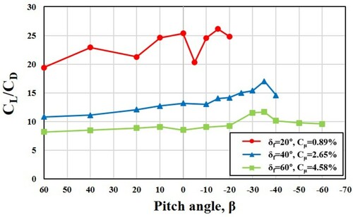
Figure 10 shows the variations of C_L/C_D with the pitch angle for the three flap angles. The smallest flap angle δ_f = 20° shows the highest C_L/C_D, and the level decreases as the flap angle increases. Overall, C_L/C_D increases with the pitch angle until the angle reaches its maximum near the negative value of the flap angle, although there are some fluctuations. In the case of δ_f = 20°, there is a sudden drop at β = −5°. This seems to occur because C_L/C_D is amplified, especially for this low flap angle, by combining the effects of the change in the oscillator location (from A to B in Figure 3) on the lift and drag. The maximum C_L/C_D occurs at β = −15° for δ_f = 20° and at β = −35° for δ_f = 40° and 60°.

Figure 10. Variations of lift-to-drag ratio with pitch angle of fluidic oscillators for different flap angles.

5.3.4. Pressure coefficient

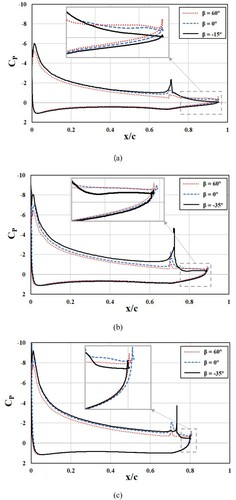
The distributions of the pressure coefficient on the airfoil for the three flap angles are shown in Figure 11. For each flap angle, the distributions are plotted for three pitch angles. Almost the same distributions are found on the lower airfoil surface regardless of the pitch angle. For each flap angle, the negative pitch angle shows the best pressure recovery and the highest lift (i.e. the largest area between the upper and lower pressure distributions) among the tested pitch angles. The highest peak of the negative pressure coefficient commonly occurs due to the injection of jets from the oscillators.

Figure 11. Distributions of pressure coefficient on airfoil surface for different pitch angles (y/s=0.5): (a) flap angle 20°, (b) flap angle 40°, and (c) flap angle 60°.

5.3.5. Analysis of flow field

Figure 12 shows the velocity contours and vectors on the x-z plane at y/s=0.5 for three flap angles. For all flap angles, the flow separation region is effectively reduced at negative pitch angles but is rather enlarged at positive pitch angles. Separation control is shown to be more effective as the flap angle decreases. As shown in the vector plots, the vortex occurring on the flap surface disappears as the pitch angle becomes negative at flap angles of 20° and 40°. At flap angles of 60°, the negative pitch angle shows remarkably reduced intensity of the vortex compared to that at β = 0°, which positively affects the aerodynamic performance. These results are consistent with the results shown in Figure 8.

Figure 12. Time-averaged streamwise velocity contours and velocity vectors for different pitch and flap angles on x-z plane at y / s = 0.5 (α = 8°).

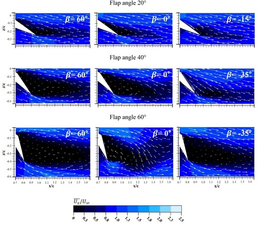
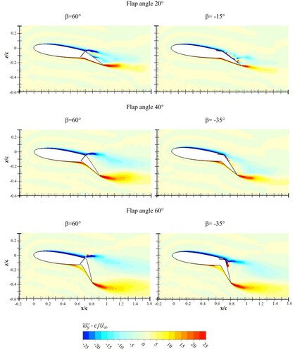
Figure 13 compares the time-averaged span vorticity distributions for different flap angles and pitch angles. It is known that positive vortices contribute to thrust, and negative vortices contribute to lift (Zha et al., 2018). Unlike the phenomena at a positive pitch angle (β = 60°), the strong vorticity generated by the jets issuing from the oscillators persists on the flap at a negative pitch angle (β = 15 or 35°), contributing to the performance. However, the vorticity strength on the flap decreases as the flap angle increases. For a positive pitch angle, the negative vorticity flow is pushed away from the flap surface by the oscillators.

Figure 13. Time-averaged spanwise vorticity contours.

6. Conclusion

The effects of the pitch angle of oscillators mounted in front of a flap on an airfoil for different flap angles were evaluated numerically. The numerical results were validated with experimental data under the same conditions. As the pitch angle (β) decreased, the lift coefficient generally increased and reached a peak value at a pitch angle close to the negative of each flap angle (δ_f). This means that the lift coefficient increased up to a certain pitch angle as the jet injection from the oscillators became more parallel to the flap. The flap angle δ_f = 20° showed remarkably larger improvement in the lift coefficient by the oscillators compared to the other flap angles in the whole pitch angle range.

The highest relative lift increment of about 30% was obtained at β = −10° for δ_f = 20°. The drag coefficient showed less variations than the lift coefficient, and the variation became larger as the flap angle increased. At δ_f = 60°, the maximum drag coefficient was found in the range of 0° ≥ β ≥ −20°. At δ_f = 40° and 60°, negative pitch angles showed lower drag coefficients less than those at the reference condition (β = 0°), so both the lift and the drag coefficients were improved. Similar maximum relative drag reductions of about 13% were obtained at β = 10° for δ_f = 20°, at β = −35° for δ_f = 40°, and at β = −30° for δ_f = 60°.

Overall, the relative drag reduction due to the oscillators was less than the relative increase in lift in all cases. The highest level of lift-to-drag ratio was obtained for the smallest flap angle, δ_f = 20°, and the level decreased as the flap angle increased. The lift-to-drag ratio generally increased with the pitch angle before reaching a peak value. The maximum lift-to-drag ratio occurred at β = −15° for δ_f = 20° and at β = −35° for δ_f = 40° and 60°. Therefore, negative pitch angles of the oscillators improved in most of the tested cases the aerodynamic performance of the airfoil compared to the reference condition and case without oscillators, but not always. The results could be helpful in selecting an appropriate pitch angle for oscillators for a flap angle or automatically adjusting the pitch angle according to the change in the flap angle.

However, in the present study, due to the geometric limitation, location of the oscillator outlets was moved downstream for negative pitch angles, resulting in the difference in the test condition. Therefore, more rigorous study is needed in the future, and the effects of bending outlet of a fluidic oscillator on the performance such as jet frequency and velocity ratio should be investigated.

Acknowledgments

This work was supported by the National Research Foundation of Korea (NRF) grant funded by the Korean government (MSIT) (No. 2019R1A2C1007657).

Disclosure statement

No potential conflict of interest was reported by the author(s).

Additional information

Funding

This work was supported by the National Research Foundation of Korea (NRF) grant funded by the Korean government (MSIT) (No. 2019R1A2C1007657).

References

- ANSYS. (2014). ANSYS CFX-Solver Theory Guide-Release 15.0. Canonsburg, PA: ANSYS Inc.
- Bardina, J. E., Huang, P. G., & Coakley, T. J. (1997). Turbulence modeling validation. 28th fluid dynamics conference.
- Celik, I. B., Ghia, U., Roache, P. J., Freitas, C. J., Coleman, H., & Raad, P. E. (2008). Procedure for estimation and reporting of uncertainty due to discretization in CFD applications. Journal of Fluids Engineering, 130(7), 078001. https://doi.org/https://doi.org/10.1115/1.2960953
- Cully, D. E., Bright, M. M., Prahst, P. S., & Strazisar, A. J. (2004). Active flow separation control of a Stator Vane using embedded injection in a multistage compressor experiment. Journal of Turbomachinery, 126(1), 24–34. https://doi.org/https://doi.org/10.1115/1.1643912
- Ghalandari, M., Shamshirband, S., Mosavi, A., & Chau, K.-W. (2019). Flutter speed estimation using presented differential quadrature method formulation. Engineering Applications of Computational Fluid Mechanics, 13(1), 804–810. https://doi.org/https://doi.org/10.1080/19942060.2019.1627676
- Hossain, M. A., Agricola, L., Ameri, A., Gregory, J. W., & Bons, J. P. (2019). Sweeping Jet film cooling on A Turbine Vane. Journal of Turbomachinery, 141(3), TURBO-18-1257. https://doi.org/https://doi.org/10.1115/1.4042070
- Jeong, H. S., & Kim, K. Y. (2018). Shape optimization of a feedback-channel fluidic oscillator. Engineering Applications of Computational Fluid Mechanics, 12(1), 169–181. https://doi.org/https://doi.org/10.1080/19942060.2017.1379441
- Jhonston, J. P., & Nishi, M. (1990). Vortex generator jets – Means for flow separation control. AIAA Journal, 28(6), 989–994. https://doi.org/https://doi.org/10.2514/3.25155
- Jones, G. S., Milholen, W. E., Chan, D. T., Melton, L., Goodliff, S. L., & Cagle, C. M. (2017). A sweeping jet application on a high Reynolds number Semispan supercritical wing configuration. 35th AIAA applied aerodynamics conference, Denver, Colorado, 5-9 June, 2017. https://doi.org/https://doi.org/10.2514/6.2017-3044
- Joshi, S. N., & Gujarathi, Y. S. (2016). A review on active and passive flow control techniques. International Journal on Recent Technologies in Mechanical and Electrical Engineering, 3(4), 1–6. https://doi.org/https://doi.org/10.2514/3.25155
- Kim, S. H., & Kim, K. Y. (2019). Effects of installation conditions of fluidic oscillators on control of flow separation. AIAA Journal, 57 (12) (2019), 5208–5219. https://doi.org/https://doi.org/10.2514/1.J058527
- Kim, S. H., & Kim, K. Y. (2020). Effects of installation location of fluidic oscillators on aerodynamic performance of an airfoil. Aerospace Science and Technology, 99, 105735. https://doi.org/https://doi.org/10.1016/j.ast.2020.105735
- Kim, S. H., Kim, H. D., & Kim, K. C. (2019). Measurement of two-dimensional heat transfer and flow characteristics of an impinging sweeping jet. International Journal of Heat and Mass Transfer, 136(2019), 415–426. https://doi.org/https://doi.org/10.1016/j.ijheatmasstransfer.2019.03.021
- Koklu, M. (2018). The effects of sweeping jet actuator parameters on flow separation control. AIAA Journal, 56(1), 100–110. https://doi.org/https://doi.org/10.2514/1.J055796
- Koklu, M., & Owens, L. R. (2014). Flow separation control over a ramp using sweeping Jet actuators. 7th AIAA flow control conference, Atlanta, GA, 16-20 Jun, 2014, pp. 16–20. https://doi.org/https://doi.org/10.2514/6.2014-2367
- Lin, J. C., Robinson, S. K., & McGhee, R. J. (1994). Separation control on high-lift airfoils via micro-vortex generators. Journal of Aircraft, 31(6), 1317–1323. https://doi.org/https://doi.org/10.2514/3.46653
- Melton, L. P. (2014). Active flow separation control on a NACA 0015 wing using fluidic actuators. 7th AIAA journal flow control conference, Atlanta, GA, 16-20 June, 2014. https://doi.org/https://doi.org/10.2514/6.2014-2364
- Melton, L. P., & Koklu, M. (2016). Active flow control using sweeping jet actuators on a semi-sapn wing model. 54th AIAA aerospace sciences meeting, San Diego, California, USA, 4-8 January, 2016. https://doi.org/https://doi.org/10.2514/6.2016-1817.
- Melton, L. P., Koklu, M., Andino, M., Lin, J. C., & Edelman, L. (2016). Sweeping jet optimization studies. 8th AIAA flow control conference, Washington, D.C., 13-17 June, 2016.
- Melton, L. P., Koklu, M., Andino, M., & Lin, J. C. (2018). Active flow control via discrete sweeping and steady jets on a simple-hinged flap. AIAA Journal, 56(8), 2961–2973. https://doi.org/https://doi.org/10.2514/1.J056841
- Menter, F. R. (1994). Two-equation eddy-viscosity turbulence models for engineering applications. AIAA Journal, 32(8), 1598–1605. https://doi.org/https://doi.org/10.2514/3.12149
- Pandey, R. J., & Kim, K. Y. (2018a). Numerical modeling of internal flow in a fluidic oscillator. Journal of Mechanical Science and Technology, 32(3), 1041–1048. https://doi.org/https://doi.org/10.1007/s12206-018-0205-x
- Pandey, R. J., & Kim, K. Y. (2018b). Comparative analysis of flow in a fluidic oscillator using large eddy simulation and unsteady reynolds-averaged navier-stokes analysis. Fluid Dynamics Research, 50(6), 23. https://doi.org/https://doi.org/10.1088/1873-7005/aae946
- Panitz, T., & Wasan, D. T. (1972). Flow attachment to solid surfaces: the Coanda effect. AIChE Journal, 18(1), 51–57. https://doi.org/https://doi.org/10.1002/aic.690180111
- Raman, G., & Raghu, S. (2004). Cavity resonance suppression using miniature fluidic oscillators. AIAA Journal, 42(12), 2608–2612. https://doi.org/https://doi.org/10.2514/1.521
- Rivir, R. B., Sondergaard, R., Bons, J. P., & Lake, J. P. (2000). Passive and active control of separation in gas turbines. Fluids 2000 conference and exhibit, Denver, CO, USA, 19-22 June, 2000, pp. 19–22. https://doi.org/https://doi.org/10.2514/6.2000-2235
- Roache, P. J. (1998). Verification of codes and calculations. AIAA Journal, 36(5), 696–702. https://doi.org/https://doi.org/10.2514/2.457
- Salih, S. Q., Aldlemy, M. S., Rasani, M. R., Ariffin, A. K., Ya, T. M. Y. S. T., Al-Ansari, N., Yaseen, Z. M., & Chau, K.-W. (2019). Thin and sharp edges bodies-fluid interaction simulation using cut-cell immersed boundary method. Engineering Applications of Computational Fluid Mechanics, 13(1), 860–877. https://doi.org/https://doi.org/10.1080/19942060.2019.1652209
- Stouffer, R. (1979). U.S. oscillating spray device. 4,151,955(1).
- Woszidlo, R. (2011). Parameters governing separation control with sweeping jet actuators. 29th AIAA Applied Aerodynamics Conference, Honolulu, Hawaii, 27-30 June, 2011. https://doi.org/https://doi.org/10.2514/6.2011-3172
- Zha, G., Yang, Y., Ren, Y., & McBreen, B. (2018). Super-lift and thrusting airfoil of co-flow jet actuated by micro-compressors. 2018 flow control Conference.