Numerical investigation on the aerodynamic resistances of double-unit trains with different gap lengths

Abstract

Double-unit trains increase passenger capacity but also increase energy consumption. Therefore, research about the aerodynamic resistance of a double-unit train is of great importance to save energy. In this study, a commercial long-marshalling high-speed train and 8 kinds of double-unit trains are used to investigate the effect of the gap length on aerodynamic resistance. The results show that the aerodynamic resistance of the double-unit train is 8.5%-12.9% larger than that of the long-marshalling train. It is the tail car (CC1 car) of the first single-unit train and the head car (CC2 car) of the second single-unit train that lead to the difference in resistance. For the double-unit trains with different gap length, the resistance increases incrementally with the gap length, which is also mainly caused by the CC1 and CC2 cars. With increases to the gap length (starting from 0 mm), the resistance of the CC1 car increases with the cremental increases in the gap lengths. The resistance of the CC2 car also gradually increases when the gap lengths become larger. The resistance of the CC1 car with a gap length of 0 mm is slightly greater than that with 25 mm.

KEYWORDS:

• Double-unit train
• long-marshalling train
• aerodynamic resistance
• gap length

1. Introduction

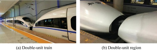
High-speed trains are gaining more and more recognition in China for their convenience and high speed. Operating mileage continues to increase, as does passenger volume (Sun et al., 2020; Tian, 2019). However, the cost of improving passenger capacity by increasing train frequency is too high, and it may increase the safety risks associated with rail transportation (Guo et al., 2018). Therefore, a double-unit train (DUT) has become an effective way to increase passenger capacity and improve passenger transportation efficiency. The double-unit train is a special train composition in which two single-unit trains are connected to increase the length. The tail car of the first single-unit train is connected to the head car of the second single-unit train, as shown in Figure 1. The area enclosed by the streamlined part of the tail car of the first single-unit train and the head car of the second single-unit train is the double-unit region.

Figure 1. Double-unit train and double-unit region.

The proposal of the DUT improves the passenger transportation efficiency. However, the presence of the double-unit region will increase aerodynamic resistance (Guo et al., 2020; Niu et al., 2017). When the running speed of a high-speed train increases, the change in aerodynamic force is more drastic. This will not only lead to more energy consumption, but also raise a series of safety concerns, such as derailment and rollover (Guo et al., 2020; Hyeokbin, 2017; Yao et al., 2015). Meanwhile, Baker’s research shows that maximum gusts could occur around the double-unit region, which may have an impact on the safety of the high-speed train operation (Baker et al., 2013). Therefore, it is very important to research the aerodynamics of DUT.

The research methods for the aerodynamic characteristic of high-speed trains include mainly numerical simulations (Medina et al., 2012; Xia et al., 2020), as well as wind tunnel experiments. Considering the cost and computational time, the numerical simulations mainly focus on the study of simple train models (Hemida & Krajnovic, 2009; Li et al., 2019), and the train models used in the numerical simulations are almost all made up of three cars (Han & Yao, 2017). Moreover, research on train drag force reduction is mainly focused on optimizing the head shape. Munoz et al. (2014), Zhang and Zhou (2013) and Choi and Kim (2014) compared the aerodynamic resistance of trains with different head shapes using wind tunnel tests, and found better aerodynamic head shapes. Zhang et al. (2017) and Sun et al. (2010)obtained excellent head shapes using multi-objective aerodynamic optimization design methods and computational fluid dynamic (CFD) simulations. For DUTs, the shape is significantly changed in the double-unit region, which makes the flow more complicated (Guo et al., 2020; Niu et al., 2017), and the double-unit region will seriously increase the resistance. It may not be enough to reduce the resistance only by optimizing the head shape. However, only a few scholars have studied multi-composition trains. As this is a special kind of multi-composition train, a study needs to be conducted on the aerodynamic characteristics around the double-unit region, and the influence of the double-unit region on train resistance. In this study, the effect of the gap length between two single-unit trains on the resistance is investigated, which provides reference materials for reducing aerodynamic resistance of DUTs.

2. Computational model and mesh

2.1. Geometry model

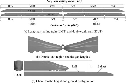
The long-marshalling train (LMT) and DUT based on a commercial high-speed train in China are established. The trains are composed of 6 individual cars. As shown in Figure 2(a), the six cars are named Head, Mid1, CC1, CC2, Mid2, and Tail respectively. 8 different gap lengths d are 0, 25, 50, 75, 100, 200, 500 and 750 mm respectively. The gap length of the DUT in operation is about 200 mm, therefore, the DUTs with a gap length equal to and less than 200 mm are selected for analysis. The main purpose of this research is to study the relationship between the resistance performance and the gap length of the train, so some DUTs with a gap length greater than 200 mm are also used for calculation, with the largest one being about 3–4 times that of the original model. Figure 2(b) is the double-unit region. Figure 2(c) shows the characteristic height H and the ground configuration. The characteristic height H defined by the distance between the rail and the roof of the train is 3.85 m. It is noted that the size described in this study is full-scale, while the models in numerical simulations are 1:8 scaled.

Figure 2. Geometry model.

2.2. Computational information

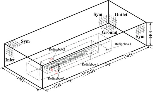
Figure 3 shows the computational domain used in the numerical simulation. The coordinate origin is located on the bottom surface of the middle car, at the intersection of the horizontal and longitudinal center planes of the middle car. 4 refinement regions are established around the model. The standard EN 14067-6:2010 stipulates the computational domain as follows: at least 8 characteristic heights upstream and 16 characteristic heights downstream. According to the standard and combined with related research, the train is placed 12H from the inlet boundary, where the incoming flow u = −97.22 m/s is applied, and 24H from the outlet boundary. The Reynolds number based on the upwind velocity and reference height H is 3.18×10⁶, and the reference height H is 1/8th scaled when calculating the Re. For the outlet boundary of the computational domain, a pressure-outlet condition is adopted, with a pressure of 0 Pa. The intensity and hydraulic diameter is chosen as the specification method for the inlet and outlet boundary, and the backflow turbulent intensity and hydraulic diameter are 0.025 and 0.481 m respectively. The upper and lateral boundaries are set as the symmetry condition, and the bottom is set as the slip wall with the speed of incoming flow. According to the research of Li et al. (2018, 2020), the k-$\omega$ SST (Shear Stress Transport) turbulence model is able to capture the airflow on the train surface. Meanwhile, the SIMPLE (Semi-Implicit Method for Pressure-Linked Equations) algorithm and the second order discretization method are adopted to obtain the flow field and pressure.

Figure 3. Computational domain.

2.3. Mesh sensitivity and validation

The model consisting of 3 cars is numerically calculated, and the result is compared with the wind tunnel experiments (Han & Yao, 2017). Models used in the numerical simulations and the wind tunnel tests are both 1/8th scaled, as shown in Figure 4. The numerical simulations use the same boundary conditions as the wind tunnel experiments, as well as the incoming flow of 60 m/s. 4 meshes, named Mesh1, Mesh2, Mesh3 and Mesh4 are generated, which contain 34.74, 27.91, 22.60 and 16.90 million cells respectively. The boundary layers of the 4 meshes are the same, consisting of 18 layers. The thickness of the first layer is 0.01 mm, and the growth ratio is 1.2. The boundary layers ensure that the y+ of the high-speed train is around 1, as displayed in Figure 5(a). Figure 5(b) shows the y+ values of every surface cell of the high-speed train in Mesh2. It can be seen that almost all cells have y+ values less than 2. The y+ values of cells are typically in the range of 0.6–1.2 except for the streamlined region of the head car and part of the bogie. Table 1 shows other details of the 4 meshes.

Figure 4 Models in the numerical simulations and wind tunnel experiments.

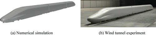
Figure 5 Results of numerical simulations and wind tunnel tests.

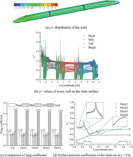
Table 1. Cell size in different regions (mm).

Mesh	Outer surface(H)	Train surface	refinebox0	refinebox1	refinebox2	refinebox3
Mesh1	200	1.56∼12.5	12.5	25	50	100
Mesh2	220	1.72∼13.75	13.75	27.5	55	110
Mesh3	260	2.03∼16.25	16.25	32.5	65	130
Mesh4	300	2.34∼18.75	18.75	37.5	75	150

The drag coefficient $C_d$ and $C_p$ are defined as (1) $\begin{array}{rl}{C}_d& =\frac{F}{0.5\rho {\mu }_{\mathrm{\infty }}^{2}A}\end{array}$(1) (2) $\begin{array}{rl}{C}_p& =\frac{p}{0.5\rho {\mu }_{\mathrm{\infty }}^2}\end{array}$(2) where $F$ is the aerodynamic force of the train, p is the pressure of the train, $\rho$ is the density of the air, ${\mu }_{\mathrm{\infty }}$ is the inlet velocity, and A is the projecting area of the high-speed train in the x direction, which is A = 10.8 m².

In the numerical simulations, the convergence criterion used is chosen through the convergence of aerodynamic forces, rather than the default residual criterion. The residual is required to be reduced to below 10⁻³–10⁻⁴, and the requirement is generally satisfied by iterating 3000 steps. However, considering the statistics of aerodynamic forces, the number of iterations is set to 6000 in this study.

The relative error in resistance coefficients of the head and tail cars for four meshes is less than 1%. The error in the drag coefficient of the middle car is about 2.3%, and that of the total train is about 2.1%. The aerodynamic resistance results of 4 meshes show that the mesh size has little effect on the aerodynamic resistance. It is observed from Figure 5(d) that the pressure distribution for three meshes of Mesh1, Mesh2 and Mesh3 is quite similar, and that the pressure coefficient at the stagnation point is about 1.0. However, the pressure coefficient of Mesh4 is different from the other three meshes in the head streamlined nose, which indicates that Mesh4 is insufficient to accurately capture the surface pressure of the train.

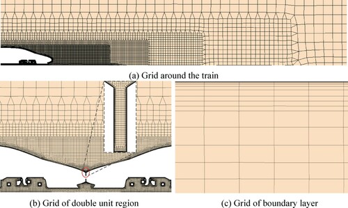
The agreement between the numerical simulations and the wind tunnel results shows that the numerical method adopted in this study can accurately simulate the aerodynamic performance of high-speed trains. Meanwhile, the agreement of the results of the drag coefficient and surface pressure coefficients indicates that Mesh1, Mesh2 and Mesh3 have sufficient accuracy. Theoretically, Mesh3 is sufficient for subsequent numerical simulations. The calculation accuracy is positively correlated with the number of cells, while too many cells will reduce the computational efficiency. Therefore, Mesh2 is chosen to conduct the subsequent research. The cell number of the DUT is about 67.0 million at this point. Figure 6(a) shows the grid around the train and the refinement zone. Furthermore, the grid of the double-unit region and the boundary layer are shown in Figure 6(b) and Figure 6(c) respectively.

Figure 6 Computational mesh.

3. Results

Numerical simulations are performed on the LMT and DUTs with different gap lengths, and the differences in aerodynamic performance between the LMT and the DUTs are investigated. Also, the impact of the gap length between two trains on the aerodynamic characteristics of DUTs is analysed.

3.1. Aerodynamic performance of the LUT and the DUT

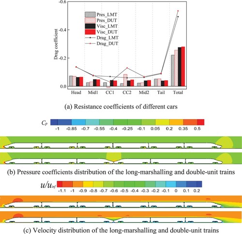
Figure 7(a) shows the drag force coefficients of the LMT and DUT. Pres_LMT stands for the pressure drag coefficient of the LMT, Visc_LMT stands for the viscous drag coefficient of the LMT, and Drag_LMT means the total resistance coefficient of the LMT. The naming convention is also suitable for DUT. Figure 7(b) and 7(c) show the pressure coefficients and velocity distribution of two types of trains at the section of y = 0 m respectively. In addition to the Head car, the resistances of the other five cars for the LMT are different from that of the DUT. As shown in Figure 7(a), the differences in the CC1 and CC2 cars of the two types of train are large, which is mostly caused by the pressure drag. The differences in Mid1, Mid2 and Tail cars are relatively small. There is no sudden change in the shape of the CC1 and CC2 cars of the LMT, therefore, the resistance shows no significant change compared with the Mid1 and Mid2 cars. For the DUT, the CC1 and CC2 cars form a double-unit region. As shown in Figure 7(b), the streamlined area of the CC1 car forms a large positive pressure when the airflow passes through this region, which reduces the negative pressure of the CC1 car or even provides positive pressure. Consequently, the pressure drag of the CC1 car reduces, which causes the resistance of the CC1 car of the DUT to be smaller than that of the LMT, as shown in Figure 7(a). The CC1 car is the tail car of Train1. Compared with the tail car of the LMU and DUT, the influence of the double-unit region on the tail car can be seen. There is also a positive pressure field with a large amplitude in the streamlined area of the CC2 car, which makes the pressure drag ofthe CC2 car increase. Therefore, the resistance of the CC1 car of DUT is smaller than that of the LMT, while the resistance of CC2 is larger. Furthermore, the pressure drag force of the Mid1 car which belongs to the DUT is bigger than that belonging to the LMT, while the viscous drag is smaller. The total resistance of Mid1 of the DUT is larger than that of the LMT.

Figure 7 Pressure and velocity distribution of two types of trains at y = 0 m.

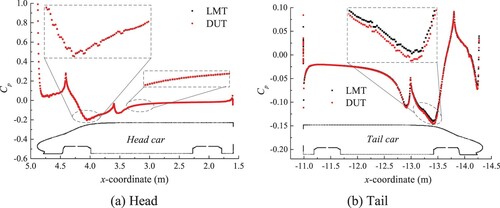
In addition to the differences in the resistance of the CC1 and CC2 cars, there is also a small difference in the resistance of the tail cars for the two types of train. The resistance of the tail car of the DUT is slightly greater than that of the LMT. Figure 8 is the pressure coefficients distribution along the upper surface of the head and tail cars for the two types of train. The surface pressure distribution of the head car is almost the same. However, there is a certain difference in the tail car, which is mainly concentrated in the streamlined area. The negative pressure on the tail of the streamline of the DUT is greater, which makes the pressure drag force of the tail car greater than that of the LMT.

Figure 8 Surface pressure coefficients of the car at a cut plane y = 0 m.

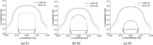
Viscous drag is also an important part of train resistance, with the magnitude of the viscous drag being positively related to the velocity near the wall. Figure 7(a) shows that the resistance pattern of the Mid2 car is similar to the Tail, and the viscous resistance is greater than that of the LMT. Taking the range of velocity less than 0.99u as the boundary layer area, the boundary layer distribution of three cross-sections are shown in Figure 9. The value in the figure is the velocity of the airflow. Figure 9 (a) shows the position of three sections in the tail car. Figure 9(b) shows the boundary layer of the tail car of the LMT, and Figure 9(c) is that of the DUT. For the cross-sections of the same train at different locations, the thickness of the boundary layer gradually increases along the train body. In order to make a clear comparison, Figure 10 shows profiles of boundary layers at each section of two trains in one image. It can be seen that the boundary layer thickness around the train of the LMT is greater than that of the DUT, which leads to the average velocity near the wall of the DUT being greater. Therefore, the viscous drag of the DUT is relatively large, which is why the resistance of the Mid2 and tail cars of DUT is greater than that of the LMT. It is worth noting that the boundary layer thickness of the DUT is greater than that of the LMT at a low height, which is caused by the development of the ground boundary layer. The turbulent airflow at the bottom of the double-unit region accelerates the development of the ground boundary layer. Therefore, the DUT has a thicker ground boundary layer.

Figure 9 Boundary layer of different cross sections of two types of trains.

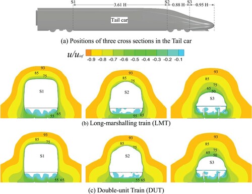
Figure 10 Velocity distribution of different cross sectionsof two types of trains.

3.2. Aerodynamic performance of the DUT with different gap lengths

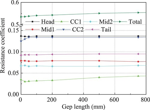
Figure 11 shows the aerodynamic resistance coefficients of each car and the whole train for DUTs with different gap lengths. The resistance of the Head and Mid1 cars are basically unchanged, which means the gap lengths only have a small effect on the cars in the front double-unit region. The drag force of the CC1 car becomes larger with increments of gap length being added to the original gap length of 0 mm. The drag force of the CC2 car also gradually becomes larger when the gap lengths increase. However, the magnitude for the CC1 car is greater than that of the CC2 car. Furthermore, the tail and Mid2 cars are less affected by the gap lengths, therefore, those resistances are almost unchanged. With the increasing increments of the gap length, the combined effect of each car makes the resistance of both Train1 and train 2 increase. However, when the gap length is more than 50 mm, the resistance of Train2 tends to be stable. To sum up, the double-unit gap length has a significant effect on the resistance of the high-speed train, and its increase will lead to an increase in the aerodynamic resistance.

Figure 11. Resistance coefficients of cars.

In order to investigate the resistance variation, the resistances of the CC1 and CC2 cars are divided into the pressure drag and viscous drag as shown in Figure 12. Figure 13 is the pressure coefficient along the upper surface of the CC1 and CC2 cars. The pressure distribution around the double-unit region at the section of y = 0 m is plotted, as shown in Figure 14.

Figure 12 Resistance of the CC1 and CC2 cars.

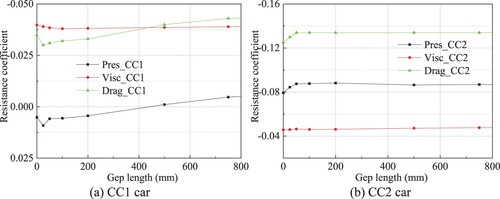
Figure 13 Surface pressure coefficients of the car at a cut plane y = 0m.

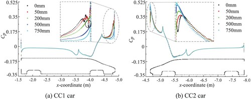
Figure 14. Pressure distribution around the double-unit region at the section of y = 0m.

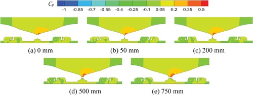
It can be found from Figure 12 that the viscous drag of the CC1 and CC2 cars are basically unaffected by the gap length. For the CC1 car, the difference in pressure distribution of DUTs with different gap lengths is mainly concentrated in the streamlined nose, and the area with high positive pressure gradually moves backward with the increase of the gap length, as shown in Figure 14. The positive pressure in the streamlined nose of the CC1 car gradually decreases, or even becomes a negative pressure, as shown in Figure 12. Therefore, the pressure drag force of the CC1 car increases, which leads to the increased resistance. For the CC2 car, the difference in the surface pressure distribution is also mainly in the streamlined nose. The amplitude of positive pressure in the tip of the nose increases rapidly as the gap length increases, whereas the pressure in the streamlined area decreases. When the gap length is small, the decrease of pressure in the streamlined area is less than the increase of pressure in the nose. Therefore, the pressure drag force of the CC2 car becomes larger. When the gap lengths reach around 50 mm, the values of reduction and increase are basically equivalent and the resistance of the CC2 car is usually stable, as shown in the Figure 12(b). When the gap length is 0 mm, the noses of the two cars are directly connected, as shown in Figure 14(a). Compared with the DUTs with a gap, there is no rear-end face for the CC1 car of a DUT with the gap length of 0 mm. It can be seen from Figure 13(a) that there is a relatively large positive pressure on the rear-end surface, which reduces the pressure drag of the CC1 car. Moreover, the streamlined area of the CC1 car forms a low pressure area that is circled with solid lines in Figure 13(a), which also leads to the increase in pressure drag force. Therefore, the resistance of the CC1 car of the DUT with the gap length of 0 mm is larger.

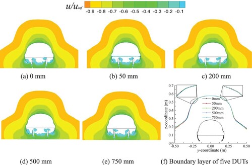
Figure 15 shows the pressure distribution along the tail car profile, and Figure 16(a)-Figure 16(e) is the boundary layer of the train at the S3 section that is shown in Figure 9(a). The pressure distribution along the upper surface of the tail cars for 5 different DUTs is almost consistent. The pressures of the body, the streamlined area and the nose are basically the same. In order to make a clear comparison, Figure 16(f) shows profiles of boundary layers at the same position of five trains in one image. It can be seen that the thickness of the boundary layer around the train of the 5 different DUTs are similar. There are only minor differences when the height is small, which is mainly due to the influence of the development of the ground boundary layer. The consistency of the boundary layer around the train body shows that the velocity distribution near the wall is consistent. Therefore, the gap length has only a small impact on the aerodynamic characteristics of the tail car of the DUT.

Figure 15. Surface pressure coefficients of the tail car at the section of y = 0 m.

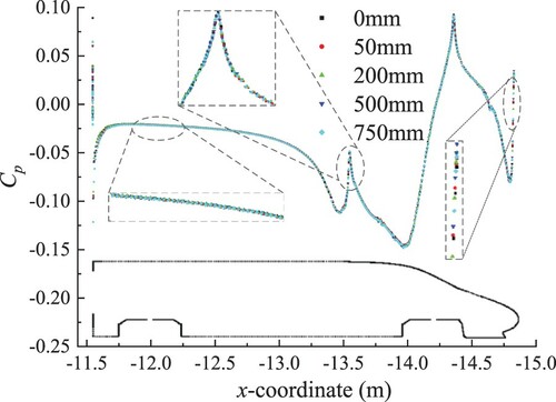
Figure 16. Boundary layer around the train at S3 cross sections for different DUTs.

4. Conclusion

In this study, the validation is conducted through the mesh sensitivity and wind tunnel tests, and the aerodynamic performance of the LMT and DUT is compared using the CFD method. Finally, the aerodynamic characteristics of DUTs with different gap lengths are investigated, and the relationship between the aerodynamic resistance and gap length is obtained. The following conclusions can be drawn from the results presented.

1. There is a significant difference in the resistance between the DUT and the LMT. The resistance of the CC1 car of the DUT is less than that of the LMT, but the resistance of CC2, Mid2 and Tail cars is greater, especially the CC2 car. As a result, the total resistance of the DUT is greater than the LMT. The resistance difference of the CC1 and CC2 cars between two types of trains is mainly caused by the pressure drag force, whereas the difference in the resistance of the Mid2 and Tail cars is mainly caused by the viscous drag force.

2. The results show that the aerodynamic resistance of the DUT is 8.5%-12.9% larger than that of the LMT. The resistances of DUTs increase with the increase of the double-unit gap length, with the changes mainly present in the CC1 and CC2 cars. The resistance of the CC1 cars of other DUTs increases as the gap lengths increase. The resistance of the CC2 cars also gradually increases when the gap length is less than 50 mm, then it gradually stabilizes.

3. The resistance of the Head and Mid1 cars are basically unchanged with the gap length increases, indicating that the gap length has no effect on the cars in the front double-unit region. For the CC1 and CC2 cars, the increases of the resistance are caused by pressure drag, whereas the gap length has little effect on the viscous drag of the CC1, CC2 and Tail cars. Furthermore, the resistance of the CC1 car of DUTs with a gap length of 0 mm is slightly greater than that of 25 mm due to the particularity of the connection form. In summary, the gap length has a significant effect on the aerodynamic resistance of the double-unit train. However, the unsteady aerodynamic and aero-acoustic characteristics of double-unit trains with different gap length are not studied in this paper. Those can be the subject of further research.

Acknowledgement

This project was supported by National Key Research and Development Program of China (No.2020YFA0710902), Sichuan Science and Technology Program (No.2019YJ0227), China Postdoctoral Science Foundation (No.2019M663550) and State Key Laboratory of Traction Power (No.2019TPLT02, TPL2005).

Disclosure statement

No potential conflict of interest was reported by the author(s).

References

- Baker, C. J., Quinn, A., Sima, M., Hoefener, L., & Licciardello, R. (2013). Full-scale measurement and analysis of train slipstreams and wakes. Part 2: Gust analysis. Institution of Mechanical Engineers Part F Journal of Rail & Rapid Transit, 228(5), 468–480. https://doi.org/https://doi.org/10.1177/0954409713488098
- Choi, J. K., & Kim, K. H. (2014). Effects of nose shape and tunnel cross-sectional area on aerodynamic drag of train traveling in tunnels. Tunnelling and Underground Space Technology, 41(3), 62–73. https://doi.org/https://doi.org/10.1016/j.tust.2013.11.012
- Guo, Z. J., Liu, T. H., Chen, Z. W., Xie, T. Z., & Jiang, Z. H. (2018). Comparative numerical analysis of the slipstream caused by single and double unit trains. Journal of Wind Engineering and Industrial Aerodynamics, 172, 395–408. https://doi.org/https://doi.org/10.1016/j.jweia.2017.11.022
- Guo, Z. J., Liu, T. H., Hemida, H., Chen, Z. W., & Liu, H. K. (2020). Numerical simulation of the aerodynamic characteristics of double unit train. Engineering Applications of Computational Fluid Mechanics, 14(1), 910–922. https://doi.org/https://doi.org/10.1080/19942060.2020.1784798
- Han, Y. D., & Yao, S. (2017). Scale effect analysis in aerodynamic performance of high-speed train. Journal of Zhejiang University (Engineering Science), 51(12), 91–99. https://doi.org/https://doi.org/10.3785/j.issn.1008-973X.2017.12.010.
- Hemida, H., & Krajnovic, S. (2009). Exploring flow structures around a simplified ICE2 train subjected to a 30° side wind using LES. Engineering Applications of Computational Fluid Mechanics, 3(1), 28–41. https://doi.org/https://doi.org/10.1080/19942060.2009.11015252
- Hyeokbin, K. (2017). A study on the resistance force and the aerodynamic drag of Korean high-speed trains. Vehicle System Dynamics, 56(8), 1–19. https://doi.org/https://doi.org/10.1080/00423114.2017.1410184.
- Li, T., Hemida, H., Zhang, J. Y., Rashidi, M., & Flynn, D. (2018). Comparisons of shear stress transport and detached eddy simulations of the flow around trains. Journal of Fluids Engineering, 140(11), 111108–12. https://doi.org/https://doi.org/10.1115/1.4040672
- Li, T., Qin, D., & Zhang, J. (2019). Effect of RANS turbulence model on aerodynamic behaviour of trains in crosswind. Chinese Journal of Mechanical Engineering, 32(85). https://doi.org/https://doi.org/10.1186/s10033-019-0402-2.
- Li, T., Qin, D., Zhang, W. H., & Zhang, J. Y. (2020). Study on the aerodynamic noise characteristics of high-speed pantographs with different strip spacings. Journal of Wind Engineering and Industrial Aerodynamics, 202, 10419. https://doi.org/https://doi.org/10.1016/j.jweia.2020.104191.
- Medina, F. A., Andres, A. S., & Grande, I. P. (2012). Gust wind tunnel study on ballast pick-up by high-speed trains. Experiments in Fluids, 52(1), 105–121. https://doi.org/https://doi.org/10.1007/s00348-011-1201-4
- Munoz, P. J., García, J., & Crespo, A. (2014). Genetically aerodynamic optimization of the nose shape of a high-speed train entering a tunnel. Journal of Wind Engineering and Industrial Aerodynamics, 130, 48–61. https://doi.org/https://doi.org/10.1016/j.jweia.2014.03.005
- Niu, J. Q., Zhou, D., Liu, T. H., & Liang, X. F. (2017). Numerical simulation of aerodynamic performance of a couple multiple units high-speed train. Vehicle System Dynamics, 55(5), 1–23. https://doi.org/https://doi.org/10.1080/00423114.2016.1277769.
- Sun, Z. X., Song, J. J., & An, Y. R. (2010). Optimization of the head shape of the CRH3 high speed train. Science China Technological Sciences, 53(12), 3356–3364. https://doi.org/https://doi.org/10.1007/s11431-010-4163-5
- Sun, Z. X., Yao, S. B., & Yang, G. (2020). Research on aerodynamic optimization of high-speed train’s slipstream. Engineering Applications of Computational Fluid Mechanics, 14(1), 1106–1127. https://doi.org/https://doi.org/10.1080/19942060.2020.1810128
- Tian, H. Q. (2019). Review of research on high-speed railway aerodynamics in China. Transportation Safety and Environment, 1(1), 1–21. https://doi.org/https://doi.org/10.1093/tse/tdz014
- Xia, Y., Liu, T. H., Gu, H. Y., & Li, L. (2020). Aerodynamic effects of the gap spacing between adjacent vehicles on wind tunnel train models. Engineering Applications of Computational Fluid Mechanics, 14(1), 835–852. https://doi.org/https://doi.org/10.1080/19942060.2020.1773319
- Yao, S. B., Guo, D. L., Sun, Z. X., & Yang, G. W. (2015). A modified multi-objective sorting particle swarm optimization and its application to the design of the nose shape of a high-speed train. Engineering Applications of Computational Fluid Mechanics, 9(1), 513–527. https://doi.org/https://doi.org/10.1080/19942060.2015.1061557
- Zhang, L., Zhang, J. Y., Li, T., & Zhang, Y. D. (2017). Multi-objective aerodynamic optimization design of high-speed train head shape. Journal of Zhejiang University Science A, 18(11), 841–854. https://doi.org/https://doi.org/10.1631/jzus.A1600764
- Zhang, Z. Z., & Zhou, D. (2013). Wind tunnel experiment on aerodynamic characteristic of streamline head of high speed train with different head shapes. Journal of Central South University, 44(6), 2603–2608. https://13-06-058.