A global analysis of a coupled violent vertical sloshing problem using an SPH methodology

Abstract

A dynamical system involving the decaying test of a partially filled liquid tank is analyzed in the present paper. This analysis is relevant for the design of aircraft fuel tanks, where the wings' structural dynamics are influenced by the complexity and the violence of the internal flow generated when atmospheric turbulence or gust is encountered. The study of this kind of system is performed in order to understand the extra energy dissipation caused by the confined fluid, and the interacting force between the fluid and the tank resulting from the vertical sloshing. A complete non-dimensional analysis of the problem in terms of additional damping has been performed, and the dependency on the most relevant non-dimensional numbers has been monitored. A coupled numerical simulation where both the tank and the fluid are combined has been used to study the system, and their results are compared to previous experiments. A smoothed particle hydrodynamics model, extensively validated in the sloshing literature, is used to calculate the magnitude and frequency of the vertical force between the fluid and the tank. The extra dissipation of the tank's mechanical energy caused by the fluid action is quantified for a particular configuration with constant filling level and a wide range of non-dimensional numbers. The sensitivity of the extra damping to the variation of the non-dimensional numbers is evaluated, and the most relevant ones are compared to the equivalent experimental tests. Results show that the numerical tool developed is able to capture the different phenomena involved and can be used to determine the influence of the different phenomena happening in violent vertically excited flows.

Keywords:

• Smoothed particle hydrodynamics
• sloshing
• viscosity

1. Introduction

The standard engineering practices for wing and aircraft design neglect the effect of fuel movement within the tanks for the determination of the aircraft design loads. Considering that aircraft wings are rather flexible structures, the movement of fuel liquid inside the tanks produces sloshing loads that can be considerably violent. These loads induce great motions in the entire wing system that can affect the overall performance if uncontrolled. It therefore seems hence beneficial to deepen the understanding of this undesirable effect.

It is possible to take advantage of the confined fluid moving within the tanks and dampen the overall energy transferred to the structure. This has motivated several investigations over the years in an attempt to accurately reproduce sloshing flows and suppress unwanted oscillations in several engineering disciplines. In other words, the purpose of all these studies is to understand the liquid sloshing motion inside a tank in order to counteract the external forces that affect the structure and dissipate energy.

Other civil infrastructures, such as large buildings or bridges, also demand some mechanical damping systems to control structural vibration. These systems are known as Tuned Liquid Dampers (TLDs), and when designed correctly allows mitigation of motions when, for example, earthquakes occur (Bulian et al., 2010; Tait, 2008). Analogously, in the naval industry similar devices are sometimes installed in the ships to reduce roll motion, known as anti-roll tanks (Souto-Iglesias et al., 2006, 2004). These ideas have been widely practiced in the last several decades and recently are being applied to aerospace rocket launches (Arndt & Dreyer, 2008). Therefore, the damping effect induced by the fluid motion can be used to control the motion of spacecraft, ships or buildings, and this idea it is also applicable to the particular case of aircraft wings.

As such, in this work the different mechanisms and physics involved in the sloshing of fluid moving inside a vertically decaying motion system are analyzed numerically, comparing the results to experimental curves. This paper complements the set of experiments performed by Martinez-Carrascal and Gonzalez-Gutierrez (2020).

Regarding experimental studies, several experimental campaigns involving SDOF systems rolling or moving horizontally have been undergone (Bouscasse et al., 2014a; Delorme et al., 2009; Moirod et al., 2011; Sun & Fujino, 1994). Conversely, the literature concerning vertical motions such as the ones presented in this work is scarce, and only a few studies have been carried out in recent decades (Bredmose et al., 2003). However, research on this topic is currently gaining attention and some recent studies can be found, such as the works by Constantin et al. (2020), Gambioli and Malan (2017), or Titurus et al. (2019) In particular, both in Constantin et al. (2020) and Titurus et al. (2019) the problem is studied from a numerical perspective to complete the experimental campaigns carried out.

There exists a set of different numerical tools that are being used to quantify the energy dissipation effects associated with the liquid movement inside confined containers undergoing dynamic excitations. The first sloshing studies were based on the potential flow theory, either using linear or nonlinear hypotheses, but nowadays most studies are conducted using the Navier–Stokes equations implemented in different CFD software (Demirbilek, 1983a, 1983b, 1983c). The biggest problem of the potential flow solution is to take into account the energy dissipation caused by viscous effects and the boundary layers. As a consequence, some additional energy dissipation terms are necessary to complement the potential flow theory (see, e.g. Antuono et al. (2012)). Most of the knowledge about sloshing and the first numerical implementations can be found in Faltinsen and Timokha (2009) and Ibrahim (2005).

Recently, analysis carried out from several authors from different disciplines have been performed, and hence similar problems has been addressed numerically with different methodologies. One of the most well-established numerical methods used is the Finite Volume Method (FVM). In order to solve satisfactorily problems involving an interface, either Volume of Fluid (VoF) or Level-Set methodologies are very popular. There are several examples that attempt to solve sloshing flows with this method, such as Gómez-Goñi et al. (2013) and Sykes et al. (2018) The main drawback found from these approaches is linked to the resolution needed to solve accurately the flow at the interface, that makes it unaffordable for certain problems. To overcome this issue, there exist a set of hybrid methods that have also been tested to solve sloshing flows. Just to cite some examples, relevant work on sloshing can be found that has been done with Particle-Finite Element Method (PFEM) by Gimenez and González (2015) or Material Point Method (MPM) by Li et al. (2014)

A different option available to solve the fluid equations numerically that arises as a powerful solution is the Smoothed Particle Hydrodynamics (SPH). SPH is a fully Lagrangian method used to solve partial differential equations. The method was conceived in 1977 (Gingold & Monaghan, 1977; Lucy, 1977) to solve astrophysics problems, but due to its flexibility it quickly spread over different disciplines, including free surface flows (Monaghan, 1994). It was a demonstrably reliable tool for solving sloshing flows, especially due to the fact that free surface boundary conditions are inherently satisfied with this methodology. Several of the most complex problems tackled in computational engineering have presented a solution only given by SPH. These problems include fluid–structure interaction problems (Stasch et al., 2016), water waves generated by landslides (Farhadi et al., 2016) and violent sloshing problems in the presence of complex geometries (Sun et al., 2019). All these research studies show the reliability of SPH in problems with a large deformation of the free surface, demonstrating its possible application in fuel sloshing simulations. Consequently, SPH presents an alternative efficient methodology compared to mesh-based methods to simulate the free surface breakage, which occurs frequently during violent sloshing. Physical phenomena such as high fragmentation and free-surface violent impacts, significantly reduce the simulation accuracy, see Banim et al. (2006). The fact that traditionally lighter phase is neglected, and only the heavier phase is modeled, is always a relevant decision to evaluate. In the kind of applications that are shown here, the density ratio between the phases is large enough ($\sim {10}^3$) to assume that this hypothesis is reasonable, allowing for a simplification of the numerical model and saving computational resources at the same time. Some of the consequences of this assumption are widely discussed by Colagrossi et al. (2009).

Similarly, as the fluids involved are assumed to be incompressible (the flow velocity is much smaller than the sound speed in water), a weakly compressible assumption is made to close the Navier–Stokes system of equations. Nevertheless, when accurate complex free-surface flows are simulated, these assumptions are not negligible at all, nor easily justified. The replacement of air with vacuum deprives the flow of cushioning mechanisms in cavities, which can significantly alter the dynamics of the flow and the energy transfer processes. Moreover, when a vacuum cavity collapses, a discontinuous drop of mechanical energy occurs (see Rogers & Szymczak, 1997) if a purely incompressible model is assumed. Conversely, in a weakly compressible model the cavity collapse induces rapid exchanges between mechanical energy and internal elastic energy (Marrone et al., 2015), which are dissipated in a few cycles by numerical viscosity. The implications of using a single-phase approximation on the simulation of energetic free-surface flows and the energy evolution, transfer and dissipation are topics still under investigation.

Different techniques have been developed in order to solve the fully coupled problem involving fluid and structural motions. For example, in Frandsen (2005) and Salih et al. (2019) the potential flow theory and the coupled Navier–Stokes equations are respectively used, whilst in the works by Yu et al. (1999) and Tait (2008) a mass-spring system is used instead. In the present work, a fully coupled system is used, which allows consideration of the extra damping that is added by the fluid's presence, either obtained experimentally or computed numerically. A similar procedure has been followed in the works by Bouscasse et al. (2014a) and Bouscasse et al. (2014b).

Hence, the aim of this work is to deepen into the understanding of a very complex flow such as the violent sloshing generated when a partially filled tank is vertically excited. Therefore, a novel large amplitude case, consisting on a highly accelerated vertical sloshing problem is studied numerically and compared to equivalent experiments in order to analyze this complex phenomena from both perspectives. Other interesting finding in this study is that these coupled problems can be described by a combination of a particle numerical method that simulates the fluid with a relatively simple model for the structural part, obtaining good agreement with experiments. A systematic wide range variation of the most relevant parameters obtained after a dimensional analysis of the problem has been performed. Experiments using different fluids confirm the results obtained numerically and provide a global perspective in order to understand the physical processes occurring in this problem.

The paper is organized as follows: first, in Section 2 the experimental rig is described, and the method to calculate the sloshing force is explained. Then, the numerical model with Smoothed Particle Hydrodynamics is presented in Section 3, including different modifications needed to simulate this vertically excited flow, and considerations concerning the coupling between the fluid and the structural solver. Once the model is presented, in Section 4 the results are shown and discussed. The different flow regimes that the fluid experiences during the test are described, and both approaches, numerical and experimental, are qualitatively described through visual comparison. Next, numerical tests are done for different resolutions with the imposed kinematics from the experiments in order to assess that SPH is a valid tool to simulate this experiment in terms of accuracy and reliability. Finally, the fully coupled system is simulated for several cases and compared to the experiments, obtaining a reasonable match between both approaches. Variation of non-dimensional numbers is explored, and some concluding remarks are drafted from the results obtained.

2. Experiments

An SDOF sloshing experimental campaign has been conducted at the Model Basin Research Group (CEHINAV) sloshing laboratory of the UPM in order to investigate the slosh-induced damping effects in Froude scaled tanks subjected to vertical accelerations.

A photograph of the experimental setup and a simplified outline are both shown in Figure 1.

Figure 1. Experimental setup and outline. (1) Load cell, (2) Metallic plate with mass, (3) Upper set of springs with stiffness constant $k_1=2160\mathrm{N}/\mathrm{m}$, (4) Lower set of springs with stiffness constant $k_2=2160\mathrm{N}/\mathrm{m}$, (5) Laser sensor, (6) Mechanical guide, (7) Accelerometer, (8) Methacrylate tank and C-shaped wooden structure with mass $m_s=2.06\mathrm{k}\mathrm{g}$, (9) Pair of solenoids acting as release mechanism. (a) Experimental setup. (b) Outline of the setup.

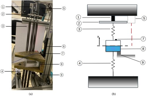
The sloshing rig is an SDOF coupled system composed of a mechanical guide that allows the 1 degree of freedom constraint. This guide is attached to a C-shaped wooden structure that holds the tank. Similarly, the C-shaped wooden structure is attached to a set of six springs (each of them having an individual spring constant of $k=720\mathrm{N}/\mathrm{m}$), three on the upper side and three on the lower side. In Figure 1(b), the upper set of springs is denoted as $k_1$ and the lower set is called $k_2$ with $k_1=k_2=3k$. The lower springs are mechanically embedded into the floor, and on the opposite side the upper set of springs is attached to a metallic plate that acts as a joint between them and the embedded load cell. The energy stored in the deformed springs is transferred to the vertical motion of the moving part of the rig. This setup also includes an accelerometer glued to the C-shaped wooden structure, a laser sensor pointing at the wooden block and two solenoids acting as a release mechanism.

The structure is deflected a certain distance $y_0$ until it is fixed by the action of both solenoids. These permanent solenoids are able to produce a magnetic force of 400 N, allowing the system to remain fixed at $y=y_0$. When the electrical current is turned on they release the structure, triggering the oscillatory movement.

The solid moving mass $m_s$ accounts for the masses of the C-shaped wooden structure, tank, mechanical bearing system and attachments, and $m_k$ represents the mass of the upper set of springs. The final list of parameters used in the SDOF experiment is presented in Table 1.

Table 1. Summary of the parameters used in the Froude scaled SDOF experimental setup.

Tank length, L [m]	0.1
Tank height, H [m]	0.06
Tank depth, B [m]	0.06
Fill level, $h_f/H$ [$\mathrm{\%}$]	50
Liquid mass $m_l$ [kg]	0.18
Solid mass $m_s$ [kg]	2.06
Spring mass $m_k$ [kg]	0.342
Total mass $m=m_s+m_l+m_k$ [kg]	2.582
K = 6k [N/m]	4320
$w_0$ [rad/s]	40.9
$f_0$ [Hz]	6.51
$y_0$ [cm]	5.9

In this experimental setup, there are three magnitudes that are being measured: the tank acceleration, the position and the load cell force. The acceleration of the moving solid mass is measured by a piezo-electric accelerometer attached to the C-shaped wooden structure close to the mechanical guide. The position and the force are measured by a single point laser sensor and a load cell respectively. Sampling frequency is set to ${10}^3$ Hz. To obtain the video frames, a camera with a maximum rate of 240 fps is used. A detailed description of the experimental setup and its characteristics is presented in Martinez-Carrascal and Gonzalez-Gutierrez (2020).

As it is explained in the work by Martinez-Carrascal and Gonzalez-Gutierrez (2020), by applying Newton's second law to bodies 1, 2 and 3 one can express the vertical projection of the sloshing force as a function of the acceleration of the tank and the measurement of the load cell, according to (1) $F_{slosh}=m_s\frac{{\mathrm{d}}^{2}y}{\mathrm{d}{t}^2}+T_{LC},$(1) where $T_{LC}=2(T-T_0)+m_k{\mathrm{d}}^{2}y/\mathrm{d}{t}^2$ represents the load cell measurement T, corrected with the static contribution $T_0$ and the springs inertia $m_k{\mathrm{d}}^{2}y/\mathrm{d}{t}^2$.

2.1. Dimensional analysis of the problem

In this section, the dimensional analysis of the problem concerning the additional damping that is obtained when a liquid phase partially fills the tank of the experimental rig described in Section 2 is performed. We are particularly interested in the rate of kinetic energy loss due to the inner fluid action.

The non-dimensional analysis will be performed for our particular experimental setup, which means that the geometry is fixed and identical to the one described in Section 2, and no geometrical scaling is performed. The decaying tests performed are well described in Martinez-Carrascal and Gonzalez-Gutierrez (2020). Using this experimental background, we can define the extra-damping $\mathrm{\Delta }\xi ={\xi }_{wet}-{\xi }_{dry}$ as the difference between the damping of the tank acceleration signals when a fluid (wet) is present inside the tank with respect to the case where there is no liquid (dry). Applying the Π theorem, this extra-damping $\mathrm{\Delta }\xi$ of the tank can be expressed as a function of the following non-dimensional numbers: (2) $\mathrm{\Delta }\xi =f\left(Re,Fr,We,Bo,\frac{h_f}{H},r,\frac{{\rho }_a}{{\rho }_f},\frac{{\mu }_a}{{\mu }_f},\frac{c}{m{\omega }_0},\frac{L}{H}\right)$(2) where ${\rho }_a$ and ${\rho }_f$ are the gas and liquid densities inside the tank, ${\mu }_a$ and ${\mu }_f$ are the gas and liquid viscosities inside the tank, m is the total mass of the system, ${\omega }_0=\sqrt{K/m}$ is the natural frequency of the system, $h_f/H$ is the filling level, $r=m_l/m_s$ represents the liquid to solid mass ratio. The rest of the non-dimensional numbers are: $F{r}^2=\frac{H{\omega }_0^2}{(a-g)}$ is square of the Froude number based on the inertial (a) and gravity (g) forces, $Re=\frac{{\rho }_f{H}^2{\omega }_0}{{\mu }_f}$ is the liquid Reynolds number, Bo is the Bond number that represents the contact angle and the meniscus height and $We=\frac{{\rho }_f{H}^3{\omega }_0^2}{\sigma }$ is the Weber number, with σ defined as the surface tension between fluids. In the dimensional analysis, ${\rho }_f{H}^3$ has been used to make the magnitudes that only refer to the fluid non dimensional, and m to do the same with the global magnitudes respectively.

As we are going to focus on our particular experimental setup, the geometry ratio $\frac{L}{H}$, the total mass m, the natural frequency of the system ${\omega }_0$ and the structural damping $\frac{c}{m{\omega }_0}$ will not be varied and we will not consider them in our analysis. Regarding the filling level f, recent studies see Constantin et al. (2020) have demonstrated that the filling level that produces a highest extra-damping is 50%. As consequence we will keep that critical filling level in our analysis in order to reduce the numerous amount of parameters of the problem. In those cases where the sloshing fluid is varied, the solid mass will be also be varied in order to maintain constant both the global mass m and the natural frequency ${\omega }_0$. Taking into account these considerations, the final expression coming from Equation (2(2) $\mathrm{\Delta }\xi =f\left(Re,Fr,We,Bo,\frac{h_f}{H},r,\frac{{\rho }_a}{{\rho }_f},\frac{{\mu }_a}{{\mu }_f},\frac{c}{m{\omega }_0},\frac{L}{H}\right)$(2) ) is simplified to (3) $\mathrm{\Delta }\xi =f\left(Re,Fr,We,Bo,r,\frac{{\rho }_a}{{\rho }_f},\frac{{\mu }_a}{{\mu }_f}\right)$(3)

3. Numerical model

The traditional SPH approach for fluid dynamics relies on a compressible formulation, assuming the fluid follows a barotropic law for pressure–density relation. With these assumptions, Navier–Stokes equations become (4) $\left\{\begin{array}{l}\frac{D\rho }{Dt}=-\rho \mathrm{\nabla }\cdot \mathit{u}\\ \frac{D\mathit{u}}{Dt}=\mathit{g}+\frac{\mathrm{\nabla }\cdot \mathbb{T}}{\rho }+{\mathit{a}}_{st}\\ \mathit{u}=\frac{\mathrm{d}\mathit{r}}{\mathrm{d}t},p=p\left(\rho \right)\end{array}\right.$(4) where $\frac{D}{Dt}$ is the Lagrangian derivative, ρ is the fluid density, $\mathit{g}$ a generic external volumetric force field, ${\mathit{a}}_{st}$ a surface force field and p the pressure. The flow velocity, $\mathit{u}$, is defined as the material derivative of a fluid particle position, $\mathit{r}$.

The stress tensor of a Newtonian fluid, $\mathbb{T}$, is defined as (5) $\mathbb{T}=(-p+\lambda \mathrm{t}\mathrm{r}\mathbb{D})\mathbb{I}+2\mu \mathbb{D},$(5) with $\mathbb{D}$ as the rate of strain tensor, i.e. $\mathbb{D}=(\mathrm{\nabla }\mathit{u}+\mathrm{\nabla }{\mathit{u}}^T)/2$; $\mathbb{I}$ the identity matrix and µ and λ the fluid viscosity coefficients.

In order to close the system of Equations in (4(4) $\left\{\begin{array}{l}\frac{D\rho }{Dt}=-\rho \mathrm{\nabla }\cdot \mathit{u}\\ \frac{D\mathit{u}}{Dt}=\mathit{g}+\frac{\mathrm{\nabla }\cdot \mathbb{T}}{\rho }+{\mathit{a}}_{st}\\ \mathit{u}=\frac{\mathrm{d}\mathit{r}}{\mathrm{d}t},p=p\left(\rho \right)\end{array}\right.$(4) ) a stiff equation of state is needed. This is how the compressibility is adjusted so that the speed of sound can be artificially lowered (Antuono et al., 2010). Normally, the linear term is sufficient to retain the properties of the EOS.

The system in Equation (4(4) $\left\{\begin{array}{l}\frac{D\rho }{Dt}=-\rho \mathrm{\nabla }\cdot \mathit{u}\\ \frac{D\mathit{u}}{Dt}=\mathit{g}+\frac{\mathrm{\nabla }\cdot \mathbb{T}}{\rho }+{\mathit{a}}_{st}\\ \mathit{u}=\frac{\mathrm{d}\mathit{r}}{\mathrm{d}t},p=p\left(\rho \right)\end{array}\right.$(4) ) turns in SPH into (6) $\left\{\begin{array}{l}\frac{\mathrm{d}{\rho }_i}{\mathrm{d}t}=-{\rho }_i\sum _j{\mathit{u}}_{ji}\cdot {\mathrm{\nabla }}_i{W}_{ij}{V}_j+h{c}_s\delta \sum _j{\mathit{\psi }}_{ji}\cdot {\mathrm{\nabla }}_i{W}_{ij}{V}_j\\ \frac{\mathrm{d}{\mathit{u}}_i}{\mathrm{d}t}=-\frac{1}{{\rho }_i}\sum _j(p_i+p_j){\mathrm{\nabla }}_i{W}_{ij}{V}_j\\ +{\mathit{g}}_i+\frac{\mu K}{{\rho }_i}\sum _j{\pi }_{ij}{\mathrm{\nabla }}_i{W}_{ij}{V}_j+{\mathit{a}}_{st}\\ \frac{\mathrm{d}{\mathit{r}}_i}{\mathrm{d}t}={\mathit{u}}_{i}p=p_0+c_s^2({\rho }_i-{\rho }_0)\end{array}\right.$(6) where ${\mathit{u}}_{ji}:=({\mathit{u}}_j-{\mathit{u}}_i)$ and $V_j$ accounts for the volume of the neighbor particles j, defined as $V_j=m_j/{\rho }_j$, and $W_{ij}=W({\mathit{r}}_j-{\mathit{r}}_i,h)$ and ${\mathrm{\nabla }}_i{W}_{ij}=\mathrm{\nabla }W({\mathit{r}}_j-{\mathit{r}}_i,h)$ represent the kernel function and its derivative with respect to the ith particle, at constant h, respectively. In this work, a Wendland C2 kernel with $h/dr=2$ is used, where h and dr correspond to the smoothing length and the particle distance respectively. The dissipation effects due to viscosity are modeled through the function ${\pi }_{ij}$, that is defined as (7) ${\pi }_{ij}:=\frac{{\mathit{u}}_{ji}\cdot {\mathit{r}}_{ji}}{\parallel {\mathit{r}}_{ji}{\parallel }^2},{\mathit{r}}_{ji}:=({\mathit{r}}_j-{\mathit{r}}_i)$(7) Alternatively, when fully turbulent regimes are developed, an LES subgrid model, such as the one presented by Di Mascio et al. (2017) and Meringolo et al. (2019), could be adopted.

In the continuity equation, an additional term is added to avoid spurious high-frequency pressure oscillations, following the work by Antuono et al. (2012). An additional term of this form has actually become a standard in SPH, and this particular model is the so called δ-SPH. The term ${\mathit{\psi }}_{ji}$ is defined as (8) ${\mathit{\psi }}_{ji}:=2\left[({\rho }_j-{\rho }_i)-\frac{1}{2}\left({〈\mathrm{\nabla }\rho 〉}_j^L+{〈\mathrm{\nabla }\rho 〉}_i^L\right)\cdot {\mathit{r}}_{ji}\right]\frac{{\mathit{r}}_{ji}}{\parallel {\mathit{r}}_{ji}{\parallel }^2}$(8) where ${〈\mathrm{\nabla }\rho 〉}_i^L$ represents the renormalized density gradient, as defined by Randles and Libersky (1996). The value for δ is set always to 0.1.

A numerical boundary integrals approach, as described by Cercos-Pita (2015) and Calderon-Sanchez et al. (2019), is used to model boundary conditions. The boundary is discretized by elements characterized by geometrical features such as their area, normal and tangent. Following this model, a truncation error is assumed. However, it avoids connectivity between nodes and allows for a more efficient computation in terms of memory and computational time savings. The Shepard factor is computed geometrically through a semi-analytical approach.

When the Reynolds number is in the order of ${10}^5$ the wall boundary layers are too thin and cannot be resolved in our simulations, hence free slip boundary conditions are used on every tank wall for those cases, unless otherwise stated.

Time integration is performed by means of a predictor-corrector scheme. Due to the violence of the impacts expected during the simulation, the Courant–Friedrichs–Lewy (CFL) condition is set to 0.1. Variable time step is used to account for the different phenomena involved, taking the minimum of the following: (9) $\begin{array}{rl}& \mathrm{\Delta }t\le \mathrm{C}\mathrm{F}\mathrm{L}\frac{h^2}{v}\mathrm{\Delta }t\le \mathrm{C}\mathrm{F}\mathrm{L}\underset{i}{min}\left(\frac{h}{c_0+h\underset{j}{max}{\pi }_{ij}}\right)\\ & \mathrm{\Delta }t\le \mathrm{C}\mathrm{F}\mathrm{L}\underset{i}{min}\left(\frac{h}{∥{\mathit{u}}_i∥}\right)\mathrm{\Delta }t\le \mathrm{C}\mathrm{F}\mathrm{L}\underset{i}{min}\sqrt{\frac{h}{∥{\mathit{a}}_i∥}}\end{array}$(9) The code used to carry out the simulations shown in this work is AQUAgpusph, an open-source SPH software developed by CEHINAV-UPM.

3.1. Additional model corrections: particle shifting and free-surface tracking

The kinds of problems that are covered in this work involve large accelerations (to the order of 10 $\mathit{g}$) that force large pressure gradients and large areas with negative gauge pressures. Simulating such dynamics is still a great challenge in SPH, mainly due to the possible appearance of numerical cavitation, which is known in SPH as tensile instability.

There are several attempts in the literature to deal with tensile instability, such as Monaghan (2000) and Sun et al. (2018). These correction terms are normally added into the momentum equation. However, in this work, a different approach is used instead that relies on the shifting technique introduced by Lind et al. (2012). Based on Sun et al. (2018) and Sun et al. (2019), a tensile instability correction term is added to the shifting law that, combined with the boundary integrals methodology, is enough to avoid numerical cavitation when large negative pressure gradients arise.

In order to overcome the undesirable effects mentioned previously and to improve the accuracy of the scheme, the Particle Shifting Technique (PST) is introduced to keep particle distribution as regular as possible. When using the PST the particles are moved with a modified velocity and therefore the system in (6(6) $\left\{\begin{array}{l}\frac{\mathrm{d}{\rho }_i}{\mathrm{d}t}=-{\rho }_i\sum _j{\mathit{u}}_{ji}\cdot {\mathrm{\nabla }}_i{W}_{ij}{V}_j+h{c}_s\delta \sum _j{\mathit{\psi }}_{ji}\cdot {\mathrm{\nabla }}_i{W}_{ij}{V}_j\\ \frac{\mathrm{d}{\mathit{u}}_i}{\mathrm{d}t}=-\frac{1}{{\rho }_i}\sum _j(p_i+p_j){\mathrm{\nabla }}_i{W}_{ij}{V}_j\\ +{\mathit{g}}_i+\frac{\mu K}{{\rho }_i}\sum _j{\pi }_{ij}{\mathrm{\nabla }}_i{W}_{ij}{V}_j+{\mathit{a}}_{st}\\ \frac{\mathrm{d}{\mathit{r}}_i}{\mathrm{d}t}={\mathit{u}}_{i}p=p_0+c_s^2({\rho }_i-{\rho }_0)\end{array}\right.$(6) ) needs to be rewritten in an Arbitrary Lagrangian Eulerian (ALE) framework. Within the latter new terms linked to the particle shifting velocity appears in the governing equations as commented in Sun et al. (2019) and further in Antuono et al. (2021). The particle shifting velocity is defined according to Sun et al. (2019) as (10) $\delta {\tilde{\mathit{u}}}_i=-U_{ref}2h\sum _j\left[1+0.2{\left(\frac{W_{ij}}{W\left(dr\right)}\right)}^4\right]{\mathrm{\nabla }}_i{W}_{ij}{V}_j$(10) The shifting velocity points towards the areas where particle distribution are irregular, and its intensity is modulated by the constant $U_{ref}\left(2h\right)$, which is problem dependent. However, in this work, a reasonable value for the reference velocity is found to be $U_{ref}=Ma\cdot c_s$. Also, a term is added to strengthen shifting capabilities to prevent tensile instability. Normally, shifting velocity keeps low enough, but a limiter condition is established just in case. (11) $\delta {\widetilde{{\mathit{u}}^{\ast }}}_i=min\left(\parallel \delta {\tilde{\mathit{u}}}_i\parallel ,\frac{U_{ref}}{4}\right)\frac{\delta {\tilde{\mathit{u}}}_i}{\parallel \delta {\tilde{\mathit{u}}}_i\parallel }$(11) Finally, shifting velocity is added to the particle velocity, and integrated in time to obtain the corrected position of the particles, such that (12) $\frac{\mathrm{d}{\tilde{\mathit{x}}}_i}{\mathrm{d}t}={\tilde{\mathit{u}}}_i+\delta {\tilde{\mathit{u}}}_i.$(12) In the presence of a free surface, shifting needs additional control. An algorithm has been developed in this regard to be applied in the region $\mathcal{F}$ close to the free surface. A similar approach to the one by Sun et al. (2018) is established: (13) $\delta {\mathit{u}}_i=\left\{\begin{array}{l}0\mathrm{i}\mathrm{f}{\lambda }_i<0.55\mathrm{a}\mathrm{n}\mathrm{d}i\in \mathcal{F}\\ {\kappa }_i\left(\mathit{I}-{\mathit{n}}_i\otimes {\mathit{n}}_i\right)\delta {\mathit{u}}_i^{\ast }\mathrm{i}\mathrm{f}{\lambda }_i\ge 0.55,{\mathit{n}}_i\cdot \delta {\mathit{u}}_i^{\ast }\ge 0\mathrm{a}\mathrm{n}\mathrm{d}i\in \mathcal{F}\\ \delta {\mathit{u}}_i^{\ast }\mathrm{i}\mathrm{f}{\lambda }_i\ge 0.55,{\mathit{n}}_i\cdot \delta {\mathit{u}}_i^{\ast }<0\mathrm{a}\mathrm{n}\mathrm{d}i\in \mathcal{F}\\ \delta {\mathit{u}}_i^{\ast }\mathrm{i}\mathrm{f}i\notin \mathcal{F}\end{array}\right.$(13) where the scalar coefficient ${\kappa }_i$ is defined as (14) ${\kappa }_i=\left\{\begin{array}{ll}0& \mathrm{i}\mathrm{f}\underset{j}{max}\left[\arccos \left({\mathit{n}}_i\cdot {\mathit{n}}_j\right)\right]\ge {15}^{\circ }\\ 1& \mathrm{o}\mathrm{t}\mathrm{h}\mathrm{e}\mathrm{r}\mathrm{w}\mathrm{i}\mathrm{s}\mathrm{e}\end{array}\right.$(14) Tracking of the free surface is computed following procedure established by Marrone et al. (2010) and Sun et al. (2019). In those works, ${\lambda }_i$ is defined as the minimum eigenvalue of the renormalization matrix defined by (15) ${\mathit{L}}_i:={\left[\sum _j{\mathit{r}}_{ji}\otimes {\mathrm{\nabla }}_i{W}_{ij}{V}_j\right]}^{-1}.$(15) Based on the values of ${\lambda }_i$, different regions can be drafted. A second step, based on the normal, is used to find the free surface particles. Normal is found according to the following expression: (16) ${\mathit{n}}_i=\frac{〈\mathrm{\nabla }\lambda {〉}_i}{∥〈\mathrm{\nabla }\lambda {〉}_i∥}\mathrm{w}\mathrm{i}\mathrm{t}\mathrm{h}〈\mathrm{\nabla }\lambda {〉}_i=-\sum _j\left({\lambda }_j-{\lambda }_i\right){\mathit{L}}_i{\mathrm{\nabla }}_i{W}_{ij}{V}_j$(16) Considerations regarding the free surface are especially challenging in the presence of solid walls, regardless of the methodology that is used to model such solid boundaries. Therefore, in order to compute the eigenvalues to calculate the normal in Equation (16(16) ${\mathit{n}}_i=\frac{〈\mathrm{\nabla }\lambda {〉}_i}{∥〈\mathrm{\nabla }\lambda {〉}_i∥}\mathrm{w}\mathrm{i}\mathrm{t}\mathrm{h}〈\mathrm{\nabla }\lambda {〉}_i=-\sum _j\left({\lambda }_j-{\lambda }_i\right){\mathit{L}}_i{\mathrm{\nabla }}_i{W}_{ij}{V}_j$(16) ), the values at the boundary need to be taken into account. This way, the normal can be computed appropriately.

However, eigenvalues to compute the shifting velocity from Equation (13(13) $\delta {\mathit{u}}_i=\left\{\begin{array}{l}0\mathrm{i}\mathrm{f}{\lambda }_i<0.55\mathrm{a}\mathrm{n}\mathrm{d}i\in \mathcal{F}\\ {\kappa }_i\left(\mathit{I}-{\mathit{n}}_i\otimes {\mathit{n}}_i\right)\delta {\mathit{u}}_i^{\ast }\mathrm{i}\mathrm{f}{\lambda }_i\ge 0.55,{\mathit{n}}_i\cdot \delta {\mathit{u}}_i^{\ast }\ge 0\mathrm{a}\mathrm{n}\mathrm{d}i\in \mathcal{F}\\ \delta {\mathit{u}}_i^{\ast }\mathrm{i}\mathrm{f}{\lambda }_i\ge 0.55,{\mathit{n}}_i\cdot \delta {\mathit{u}}_i^{\ast }<0\mathrm{a}\mathrm{n}\mathrm{d}i\in \mathcal{F}\\ \delta {\mathit{u}}_i^{\ast }\mathrm{i}\mathrm{f}i\notin \mathcal{F}\end{array}\right.$(13) ) do not consider the extension on the boundary. This way, the tips are correctly identified and the simulation remains stable.

3.2. Surface tension model

A general surface tension field ${\mathit{a}}_{st}$ is added to the momentum equation in Equation (6(6) $\left\{\begin{array}{l}\frac{\mathrm{d}{\rho }_i}{\mathrm{d}t}=-{\rho }_i\sum _j{\mathit{u}}_{ji}\cdot {\mathrm{\nabla }}_i{W}_{ij}{V}_j+h{c}_s\delta \sum _j{\mathit{\psi }}_{ji}\cdot {\mathrm{\nabla }}_i{W}_{ij}{V}_j\\ \frac{\mathrm{d}{\mathit{u}}_i}{\mathrm{d}t}=-\frac{1}{{\rho }_i}\sum _j(p_i+p_j){\mathrm{\nabla }}_i{W}_{ij}{V}_j\\ +{\mathit{g}}_i+\frac{\mu K}{{\rho }_i}\sum _j{\pi }_{ij}{\mathrm{\nabla }}_i{W}_{ij}{V}_j+{\mathit{a}}_{st}\\ \frac{\mathrm{d}{\mathit{r}}_i}{\mathrm{d}t}={\mathit{u}}_{i}p=p_0+c_s^2({\rho }_i-{\rho }_0)\end{array}\right.$(6) ) to deal with effects happening at the interface, and account for their contribution to the overall balance, as it has been included as a relevant physical phenomenon in Section 2.1.

This force has been included in SPH in the same fashion as in Morris (2000), and the expression reads: (17) ${\mathit{a}}_{st}=-\frac{\sigma }{{\rho }_i}\sum _j({\mathit{n}}_j-{\mathit{n}}_i)\cdot \mathrm{\nabla }{W}_{ij}{V}_j{\mathit{n}}_i$(17)

3.3. Sloshing force and fluid structure interaction

The equation that rules the vertical motion of the tank can be modeled by the application of Newton's second law to the solid mass $m_s$, and assuming that different forces are applied to the tank in the same fashion as it is derived in Martinez-Carrascal and Gonzalez-Gutierrez (2020). These forces can be split up into three components: the spring forces $-Ky$, the vertical component of the sloshing force coming from the internal fluid action $F_{slosh}$ and the vertical component of the damping force $F_D=B_{0d}\mathrm{s}\mathrm{i}\mathrm{g}\mathrm{n}\left(\mathrm{d}y/\mathrm{d}t\right)-B_{1d}\mathrm{d}y/\mathrm{d}t$. This last damping component is assumed to cause all sources of energy dissipation in the tank movement that are not due to fluid slosh, and it is composed of a Coulomb friction and viscous friction term: (18) $F_{slosh}-B_{0d}\cdot sign\left(\frac{\mathrm{d}y}{\mathrm{d}t}\right)-B_{1d}\cdot \frac{\mathrm{d}y}{\mathrm{d}t}-K\cdot y=m_s\frac{d^{2}y}{\mathrm{d}{t}^2}$(18) where $B_{0d}=0.38$ N represents the Coulomb damping coefficient and $B_{1d}=1.73$ kg/s is the viscous damping coefficient, both determined experimentally in dry tests. The vertical sloshing force $F_{slosh}$ is given, for a Newtonian fluid, by (19) $F_{slosh}=-{\int }_{S_{tank}}p\mathbf{n}\mathrm{d}S+2\mu {\int }_{S_{tank}}\mathbb{D}\mathbf{n}\mathrm{d}S$(19) The two terms in which this force is split represent the contribution of the pressure and the viscosity forces, $S_{tank}$ is the top and bottom internal surfaces of the tank, $\mathbf{n}$ is the normal vector to the surfaces pointing away from the fluid, $\mathbb{D}$ is the fluid velocity strain rate tensor, and µ is the dynamic viscosity of the fluid. In SPH, $F_{slosh}$ can be computed on the boundary elements (BE) according to the following expressions: (20) $\begin{array}{rl}{F}_{slosh}^p& =-\sum _i\sum _{j\in BE}\left(p_j+p_i\right){\mathbf{n}}_j{W}_{ij}{V}_i{S}_j,\\ F_{slosh}^V& =\mu \sum _i\sum _{j\in BE}\left[{\pi }_{ij}{\mathbf{n}}_j+\frac{\left(\mathit{I}-{\mathit{n}}_j\otimes {\mathit{n}}_j\right){\mathit{u}}_{ji}}{\mid {\mathit{r}}_{ij}\cdot {\mathit{n}}_j\mid }\right]W_{ij}{V}_i{S}_j,\end{array}$(20) where the second term of the viscous force $F_{slosh}^V$ is accounted only in case no slip boundary conditions are enforced. A similar procedure to compute the forces is followed by Chiron et al. (2019)

In AQUAgpusph, the vertical motion of the tank is obtained from the solution of Equation (18(18) $F_{slosh}-B_{0d}\cdot sign\left(\frac{\mathrm{d}y}{\mathrm{d}t}\right)-B_{1d}\cdot \frac{\mathrm{d}y}{\mathrm{d}t}-K\cdot y=m_s\frac{d^{2}y}{\mathrm{d}{t}^2}$(18) ) with the force obtained from the application of Equation (20(20) $\begin{array}{rl}{F}_{slosh}^p& =-\sum _i\sum _{j\in BE}\left(p_j+p_i\right){\mathbf{n}}_j{W}_{ij}{V}_i{S}_j,\\ F_{slosh}^V& =\mu \sum _i\sum _{j\in BE}\left[{\pi }_{ij}{\mathbf{n}}_j+\frac{\left(\mathit{I}-{\mathit{n}}_j\otimes {\mathit{n}}_j\right){\mathit{u}}_{ji}}{\mid {\mathit{r}}_{ij}\cdot {\mathit{n}}_j\mid }\right]W_{ij}{V}_i{S}_j,\end{array}$(20) ). The equation is integrated in time by means of a fourth-order Runge–Kutta integrator (RK4) to obtain the acceleration, velocity and position that are set to the boundary elements that compound the tank. This exchange of information is done at every time step, provided that the explicit scheme that SPH uses implies much smaller time steps than the ones given by the limitations of the RK4 in the tank equation Equation (18(18) $F_{slosh}-B_{0d}\cdot sign\left(\frac{\mathrm{d}y}{\mathrm{d}t}\right)-B_{1d}\cdot \frac{\mathrm{d}y}{\mathrm{d}t}-K\cdot y=m_s\frac{d^{2}y}{\mathrm{d}{t}^2}$(18) ). This difference assures the stability of the coupled system.

4. Results and discussion

In this section, the results obtained for the coupled numerical damped-mass-spring-SPH code, and the comparisons with the experiments, are presented. Previous free surface validation of the SPH method in less violent rotating coupled systems can be found in Bouscasse et al. (2014a) and particular applications of AQUAgpusph in this context are also shown in e.g. Bulian and Cercos-Pita (2018) and Serván-Camas et al. (2016).

First, in order to understand the complexity of the flow involved in the problem, a complete description of the evolution of the flow during the experiment will be laid out. Before the discussion about the coupled system results, a validation of the SPH model described in Section 3 will be presented. In order to validate the fluid SPH solver exclusively, the system will be uncoupled, and the tank movement will be externally prescribed, where the input motion imposed comes from previous experimental records.

In order to study the dependence of the sloshing problem on the fluid used, four different fluids are used inside the tank, see Table 2. Depending on the fluid used for the experiment the Reynolds number changes from Re = 130, corresponding to the glycerine, to $Re=3.8\cdot {10}^5$, which corresponds to acetone. In all the fluids tested, there exists a critical Reynolds number $R{e}_c$ that separates the laminar and the turbulent regimes. It will be observed that fluids behave differently, in terms of sloshing action, depending on the Reynolds number at which the experiment is carried out.

Table 2. Physical properties and characteristic Reynolds number of the fluids used in the experiments.

Liquid	$\rho \left[\mathrm{k}\mathrm{g}/{\mathrm{m}}^3\right]$	$\mu [\mathrm{P}\mathrm{a}\cdot \mathrm{s}]$	$Re=\rho U\mathrm{L}/\mu$	$\sigma \left[\mathrm{m}\mathrm{N}/\mathrm{m}\right]$
Water	998	8.9$\cdot {10}^{-4}$	1.6$\cdot {10}^5$	72.7
Oil	900	4.5$\cdot {10}^{-2}$	3000	33
Acetone	791	3.1$\cdot {10}^{-5}$	3.8$\cdot {10}^5$	23.7
Glycerine	1262	1.49	130	64

All the numerical tests carried out in this work correspond to a 2D configuration and a single-phase fluid model where only the heavier fluid has been considered. This is in contrast to the experimental setup, where 3D effects are present and air is the lighter fluid in all the cases.

For this particular SPH study, we just consider a single liquid phase inside the tank, and therefore, the non-dimensional expression for the additional damping caused by the liquid presence can be simplified from the one derived in Section 2.1, neglecting the two non-dimensional numbers involving the air density and viscosity. Thus Equation (3(3) $\mathrm{\Delta }\xi =f\left(Re,Fr,We,Bo,r,\frac{{\rho }_a}{{\rho }_f},\frac{{\mu }_a}{{\mu }_f}\right)$(3) ) turns into: (21) $\mathrm{\Delta }\xi =f(Re,Fr,We,Bo,r)$(21) It is an important goal of this paper to investigate how sensitive the extra damping to these five non-dimensional numbers is. The best methodology to perform this task is the computational one, which allows varying a single non-dimensional number while the rest can remain unaltered. This possibility is hard to perform experimentally.

4.1. Flow description

In this section, we want to describe the main characteristics of such a violent flow as the one generated inside the tank during the experiments described in Section 2. The dynamics of the flow can be split into three stages: first, flow evolution until the first impact on the upper wall where the free surface can be tracked; second, highly turbulent and shaken flow with several impacts against the top and bottom walls; and finally, a stationary wave that moves horizontally without any roof impact. For the lower viscosity fluids, such as water or acetone, the tank stops while the fluid is still clearly oscillating.

Let us describe these stages in more detail for a clearly turbulent case, which are the most similar cases to those like the fuel carried in aircraft tanks. The description will be done with a water test, and snapshots of both the experiment and the simulation at different stages will be shown. Figure 2 shows the tank position, velocity and acceleration for the water case during the first stage of the SPH simulation. This kinematic description of the flow comes from the filtered acceleration and position signals measured during the experiment, while the velocity is computed numerically.

Figure 2. Position, velocity and acceleration imposed to the tank during the first stage of the SPH experiment.

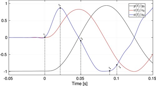
4.1.1. Stage 1

The initial setup in the experiment, before the tank is accelerated upwards, corresponds to the fluid at rest with a hydrostatic pressure distribution and a meniscus that can be found close to the boundaries due to surface tension. In this situation, the maximum pressure is found at the bottom of the tank with a value $p_0=\rho g{h}_f$. In the SPH simulation, the meniscus is imposed artificially by adding a set of particles with the desired contact angle and meniscus height. Once the upwards acceleration starts at $t_1=0\mathrm{s}$, the inertial force comes into play, and it is added to the gravity force, breaking the initial meniscus equilibrium. This instability at the free surface generates a horizontal wave that travels from the boundaries towards the tank center, as it is depicted in Figure 3. In terms of stability analysis, an unstable mode appears at the meniscus region and moves horizontally perturbing the free surface. The acceleration reaches a maximum value $a/a_0=0.87$ at time $t_1=0.021\mathrm{s}$ when the tank is still moving upwards. Note that accelerations are normalized with $a_0=9.56\mathrm{g}$. The acceleration starts to decrease until it changes sign, and at a certain instant $t_3=0.05\mathrm{s}$ is opposed and greater than gravity, $a/a_0=-0.1$. In this situation, a Rayleigh–Taylor instability (RTI) is generated that excites all the free surface, showing the characteristic finger shapes. The evolution of this double instability effect, caused by the RTI and the meniscus, generate a characteristic triple air pocket and double jet image, found in this particular case at time $t_4=0.09\mathrm{s}$ (see Figure 4). It is important to underline that without the inclusion of the meniscus in the numerical simulation the free surface evolution is considerably different, and the pocket/jet image is never obtained, as it will be shown in Section 4.3.1. The first stage finishes when the first roof impact is observed. This jet impact appears at time $t_5=0.1\mathrm{s}$, when the tank is moving downwards, and the maximum pressure value obtained in the SPH simulation is increased by about two orders of magnitude when the maximum value is compared before and after the impact ($p_1^{-}\simeq 5.5\cdot {10}^2$ Pa versus $p_1^{+}\simeq 2\cdot {10}^4$ Pa). The maximum water jet velocity before the impact can be measured numerically, being the vertical velocity at the top of the jet $v_{jet}=1.67\mathrm{m}/\mathrm{s}$, that is less than the maximum velocity limit at which the tank is moved, $v_{tank}=2\mathrm{m}/\mathrm{s}$.

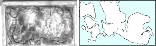
Figure 3. Free surface horizontal wave created by the meniscus presence that travels from the boundaries towards the tank center. Comparison between the experiment (left) and the SPH simulation (right).

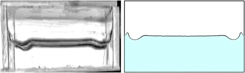
Figure 4. Characteristic triple air pocket and double jet image, typically found at time $t_4=0.09$.

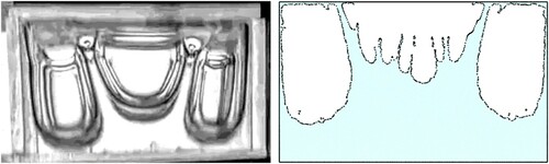
4.1.2. Stage 2

The second stage starts after the first impact $t>t_5$ and it is characterized by several violent impacts between the upper and lower walls of the tank and the fluid. During this time, a highly turbulent and violent flow is observed, where the free surface is extremely difficult to identify (see Figure 5). During this stage, integral quantities such as the vertical sloshing force can be compared between experiments and numerical simulations. This stage finishes when the last water-roof impact is observed at time $t_6=2.84\mathrm{s}$.

Figure 5. Snapshots of the turbulent and violent stage, where the free surface is hardly identified.

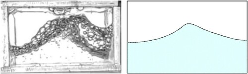
4.1.3. Stage 3

Finally the third stage comprises the times where the tank movements are negligible compared to the liquid ones for little viscosity fluids. In these cases, the fluid still moves from left to right and vice versa, tending to its natural sloshing frequency while the tank is stopped (see Figure 6). The frequency measured in this last part is around $\omega =31.16\mathrm{r}\mathrm{a}\mathrm{d}/\mathrm{s}$, not far from the characteristic sloshing frequency ${\omega }_1=28.18\mathrm{r}\mathrm{a}\mathrm{d}/\mathrm{s}$.

Figure 6. Snapshots of the standing wave stage, where the free surface is well identified.

4.2. SPH validation: forced case

In this section, a validation of the SPH code in this violent vertical sloshing context is presented. For this particular case, the structural problem is decoupled from the fluid computation. Consequently, experimental motion record obtained from the experiments will be used, instead of Equation (18(18) $F_{slosh}-B_{0d}\cdot sign\left(\frac{\mathrm{d}y}{\mathrm{d}t}\right)-B_{1d}\cdot \frac{\mathrm{d}y}{\mathrm{d}t}-K\cdot y=m_s\frac{d^{2}y}{\mathrm{d}{t}^2}$(18) ) presented in Section 3.3. The projection of the force between the fluid and the tank walls on the vertical direction $F_{slosh}$ computed by the SPH code will be compared to the experimental signal for the four different fluids. The force is computed by numerical integration of the pressure forces and the viscous stress tensor on the inner tank surface according to the expression (20(20) $\begin{array}{rl}{F}_{slosh}^p& =-\sum _i\sum _{j\in BE}\left(p_j+p_i\right){\mathbf{n}}_j{W}_{ij}{V}_i{S}_j,\\ F_{slosh}^V& =\mu \sum _i\sum _{j\in BE}\left[{\pi }_{ij}{\mathbf{n}}_j+\frac{\left(\mathit{I}-{\mathit{n}}_j\otimes {\mathit{n}}_j\right){\mathit{u}}_{ji}}{\mid {\mathit{r}}_{ij}\cdot {\mathit{n}}_j\mid }\right]W_{ij}{V}_i{S}_j,\end{array}$(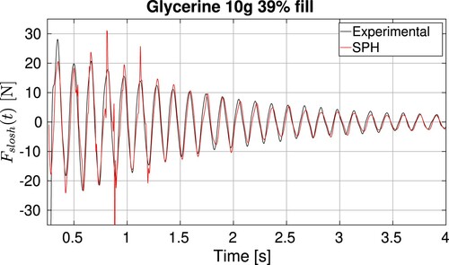20) ). The experimental and the SPH computations of the force are compared in Figure 7 for the most turbulent cases such as water, acetone and oil when the filling level is 50% and initial acceleration of $10\mathrm{g}$, and in Figure 8 for the glycerine when the filling level is 39% and also $10\mathrm{g}$. Both signals are filtered with a fourth-order Butterworth filter with a cutoff frequency of $f_0=50\mathrm{H}\mathrm{z}$. These signals contain a dominant frequency that is $6.5\mathrm{H}\mathrm{z}$. 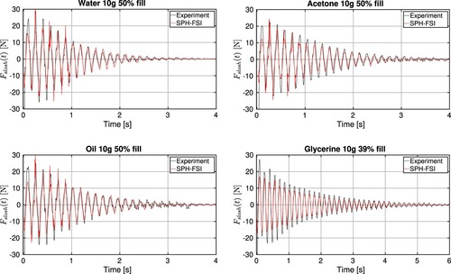From the force records presented in Figure 7, it is immediately noticeable that SPH computed force matches the experimental response for such a violent flow as the one studied here, suggesting that the dynamics originated by this violent impacting behavior is well resolved for the SPH formulation at hand. Nevertheless, some discrepancies at the peak values can be found, especially at the initial stages. From the numerical point of view, such differences are probably due to the single phase assumption, as the gas phase is important at the first vertical impact, when RTI develops. It is important to notice that no additional tensile instability correction is needed. This is a very common issue that arises in SPH when strong negative gauge pressures are involved, such as in the first stages of these computations, due to the strong sudden acceleration that is imposed to the tank. Normally, when this correction is not included in classical SPH implementations, the fluid entirely separates from the lower surface upon release, and a bulk impact with the top surface occurs for the first peak. In our case, the combination of the boundary integral formulation for the walls, the surface tension and the shifting technique was enough to avoid that hammer effect. Additionally, the initial meniscus height and the contact angle that are imposed might also play a role, as it is difficult to determine their values experimentally. Finally, 3D effects may also have an influence that justify the differences. From an experimental point of view, the errors in the first peak of the accelerometer measurements and the lack of synchronization of the two solenoids observed with the high speed camera are possible sources of experimental uncertainties.

Figure 7. Comparison of the sloshing forces computed by the SPH code versus the experiments for the forced case when different fluids at 50% filling level. From top to bottom: water, acetone and oil.

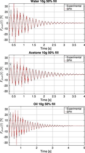
Figure 8. Comparison of the sloshing forces computed by the SPH code versus the experiments for the forced case when glycerine is used with 39% of filling level.

An influence of the number of particles in the overall force register is carried out in order to assure the accuracy of the SPH computation (see Figure 9). As it can be observed in Figure 10, the energy dissipated by the sloshing force $E_{slosh}\left(t\right)={\int }_0^t{F}_{slosh}\cdot v_{tank}\mathrm{d}t$ is not very sensitive to the number of particles used in the simulation. Indeed when the number of particles is increased from $n_y=100$ to $n_y=200$, the energy computed by the SPH code remains quite similar and always close to the experimental result.

Figure 9. Convergence test for the sloshing force computed by the SPH code for the forced case when water is used with 50% of filling level. The experimentally measured sloshing force has been included as a comparison.

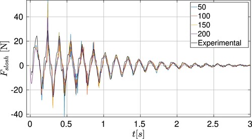
Figure 10. Convergence test for the dissipated energy by sloshing force computed by the SPH code for the forced case when water is used with 50% of filling level. The experimentally derived dissipated energy has been included as comparison.

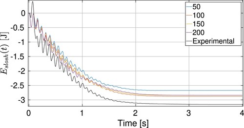
All SPH simulations were performed on a single GPU card that belongs to the CFMS computing center in Bristol UK. The 50% filling level case presented here requires a wall clock time of 5 h and 43 min to achieve 6 s of simulation time using $n_y=100$ fluid particles in the initial vertical direction. The cases with 50, 150 and 200 fluid particles require approximately 1.6, 20 and 42 h respectively. Courant number has been set to 0.1 for all the cases to ensure the stability of the numerical solution.

4.3. Fluid structure interaction problem

In this section, the results of the coupled FSI problem are presented. Consequently, both Equation (18(18) $F_{slosh}-B_{0d}\cdot sign\left(\frac{\mathrm{d}y}{\mathrm{d}t}\right)-B_{1d}\cdot \frac{\mathrm{d}y}{\mathrm{d}t}-K\cdot y=m_s\frac{d^{2}y}{\mathrm{d}{t}^2}$(18) ), which rules the tank dynamics, and the SPH fluid model run interactively. In this coupled context, not only the sloshing force $F_{slosh}$ computed is compared to the experimental signal for all fluids but also the resulting velocity of the moving tank and the damping ratio associated to the acceleration signal are quantified.

As was described in Section 2, when the complete coupled mechanical system is represented, the initial spring energy is partially transformed into both the tank and fluid mechanical energy. Every subsystem interchanges and dissipates its mechanical energy: the tank by means of aerodynamic drag and mechanical friction, whilst the fluid does so through the dissipation mechanisms embedded into the numerical model, represented by both physical and numerical dissipation terms. In particular, the power balance for the tank, obtained by the scalar product of Equation (18(18) $F_{slosh}-B_{0d}\cdot sign\left(\frac{\mathrm{d}y}{\mathrm{d}t}\right)-B_{1d}\cdot \frac{\mathrm{d}y}{\mathrm{d}t}-K\cdot y=m_s\frac{d^{2}y}{\mathrm{d}{t}^2}$(18) ) by the tank velocity, can be expressed as (22) ${\dot{E}}_{springs}-{\dot{E}}_{slosh}-{\dot{E}}_{mec,diss}={\dot{E}}_m$(22) where ${\dot{E}}_{springs}$ is the springs' power, ${\dot{E}}_m$ the tank mechanical energy, ${\dot{E}}_{slosh}$ and ${\dot{E}}_{mec,diss}$ are the power coming from the fluid sloshing action and the power dissipated by both the tank aerodynamic drag and mechanical friction respectively.

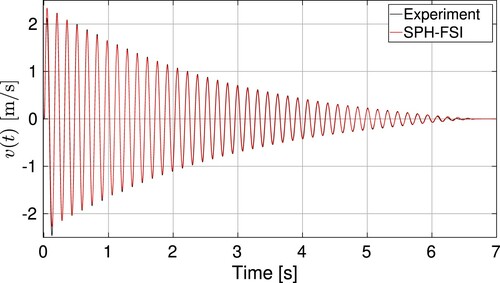
Figure 11 shows the results of the dry test case, which is carried out without the presence of fluid. The experimental evolution of the tank velocity is compared to the numerical simulation carried out solving Equation (18(18) $F_{slosh}-B_{0d}\cdot sign\left(\frac{\mathrm{d}y}{\mathrm{d}t}\right)-B_{1d}\cdot \frac{\mathrm{d}y}{\mathrm{d}t}-K\cdot y=m_s\frac{d^{2}y}{\mathrm{d}{t}^2}$(18) ). As can be observed, there exists a very good correlation between both curves, indicating that the equation used to model the mechanical system is working correctly.

Figure 11. Comparison between experimental and numerical curves for the dry test case, in which fluid is not present.

The same four fluids that have been tested for the validation forced case are also tested with an FSI approach. In Figure 12, the evolution of the tank velocity is compared to the integration of the tank acceleration measured in their corresponding experimental tests and filtered with a cutoff frequency of $f_0=50$ Hz. In Figure 13, the evolution of the sloshing force is compared to the result of the experimental expression (19(19) $F_{slosh}=-{\int }_{S_{tank}}p\mathbf{n}\mathrm{d}S+2\mu {\int }_{S_{tank}}\mathbb{D}\mathbf{n}\mathrm{d}S$(19) ) measured by the load cell and the accelerometer, where both signals are filtered using a cutoff frequency of $f_0=50$ Hz. As can be observed, for the water, acetone and oil cases both the tank velocity and the sloshing force match well with their respective experimental counterparts, where only some discrepancies in the first upper peaks can be found, in the same fashion as for the forced case. We should remark that, in the glycerine case, due to the reduced characteristic Reynolds number, the slip boundary condition used for the rest of the fluids was replaced by a no slip boundary condition that improves the approximation Colagrossi et al. (2008). Glycerin has the largest viscosity among all fluids and hence the relevance of viscous effects is expected, especially when impacts at the top disappear, and a laminar standing wave regime dominates the flow. Despite the fact that the match for the dry test reported in Figure 11 is excellent, the discrepancies between the experimental and the FSI-SPH results that still appear in Figures 12 and 13 indicate that the structural model can be improved when the fluid is added. A small lag between experimental and numerical curves can be observed at later stages for all the tests that are carried out. Also, the simplicity of the damping term of Equation (18(18) $F_{slosh}-B_{0d}\cdot sign\left(\frac{\mathrm{d}y}{\mathrm{d}t}\right)-B_{1d}\cdot \frac{\mathrm{d}y}{\mathrm{d}t}-K\cdot y=m_s\frac{d^{2}y}{\mathrm{d}{t}^2}$(18) ), and in particular its linear contribution, might play a role in the final stages. A more complex damping model, where variable coefficients are used in the structural model would help in the future to clarify if the damping model is responsible for the differences observed. Additionally, a significant air entrapment has been experimentally observed for the glycerine case. As gas phase contribution is not modeled in this work, the lack of it could also be a secondary source of the mismatch between both signals.

Figure 12. Comparison of the evolution of the tank velocity when the FSI computation is compared with the experiments for different fluids: top left, water case with 50% filling level; top right, acetone case with 50% filling level; bottom left, oil case with 50% filling level; bottom right, glycerine case with 39% filling level.

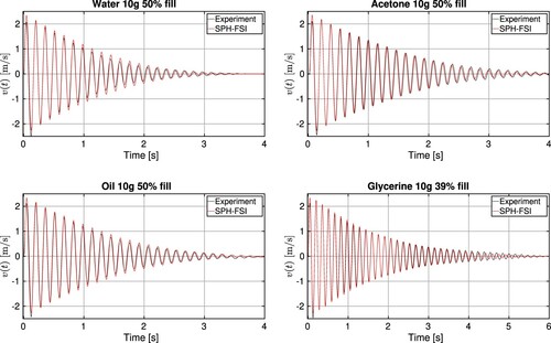
Figure 13. Comparison of the evolution sloshing force when the FSI computation is compared with the experiments for different fluids: top left, water case with 50% filling level; top right, acetone case with 50% filling level; bottom left, oil case with 50% filling level; bottom right, glycerine case with 39% filling level.

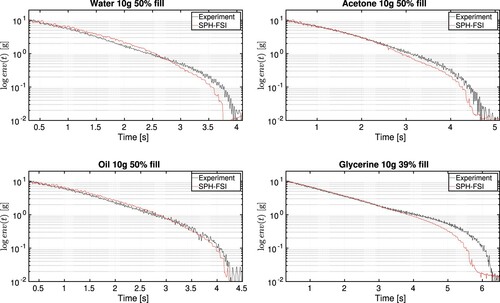
Finally, in order to compare these results in terms of dissipation, the logarithm of the envelope of the tank acceleration curves is represented in Figure 14 for all cases. The FSI-SPH numerical results are compared to its experimentally derived version, generally showing a good matching, where both numerical and experimental signals have been filtered using a cutoff frequency of $f_0=50$ Hz. The slopes of these curves represent the different regimes that can be observed, which with the exception of the glycerine, is only one regime. An interesting observation comes from the glycerine case where the experimental curve shows a slope change at time $t\approx 3.2\mathrm{s}$ which is not predicted by the numerical result. In contrast to the other fluid tests, the lack of turbulent regime in the glycerine case makes the fluid need more time to dampen the tank motion, changing the behavior of the experiment. Therefore, it is possible that FSI-SPH model is not accurately capturing the last flow evolution.

Figure 14. Comparison of the evolution of the of the decay envelope of the acceleration signal in logarithmic scale when the FSI computation is compared with the experiments for different fluids: top left, water case with 50% filling level; top right, acetone case with 50% filling level; bottom left, oil case with 50% filling level; bottom right, glycerine case with 39% filling level.

In the following sections, several SPH simulations will be carried out, changing the non-dimensional quantities that have been identified as the relevant ones in Section 2.1.

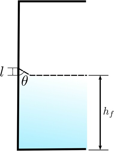
4.3.1. Bond number dependence

As it has been described in Section 4.1, influence of contact angle might be important at first stages, when instability develops before the first impact. The contact angle θ and the meniscus height l are part of the solution of the surface tension problem, see Batchelor (1973). Assuming the simplified solution where the slope of the initial free surface is everywhere small, the relation can be expressed as (23) $l=\cot \theta \sqrt{\frac{\sigma }{{\rho }_{f}g}}$(23) In this local problem, we define the Bond number using the meniscus length, and we can relate it to the contact angle as $Bo={\rho }_{f}g{l}^2/\sigma ={\cot }^2\theta$. The particular Bond number corresponding to the reference case $\theta ={45}^{\circ }$ is designated as $B{o}_0$. A detailed view of the relation between the contact angle θ and the meniscus height l can be observed in Figure 15.

Figure 15. 2-D sketch of the tank geometry used. Detail of the meniscus definition.

In this section, several computational tests have been performed changing only the contact angle between the fluid and the wall from 30 to 90 degrees, and adding particles to fill the triangular meniscus regions according to Equation (23(23) $l=\cot \theta \sqrt{\frac{\sigma }{{\rho }_{f}g}}$(23) ). This study is purely numerical, as contact angle is determined by the properties of the fluid that is tested experimentally, and its influence is normally neglected at the expense of other more relevant quantities.

The differences between the different simulations in terms of the tank velocity can be observed in Figure 16. As it can be appreciated, a clear influence of the meniscus on the overall dynamics of the experiment does not exist.

Figure 16. Comparison of the evolution of the velocity of the tank with FSI computations for $\theta ={30}^{\circ }$, $\theta ={45}^{\circ }$, $\theta ={60}^{\circ }$ and $\theta ={90}^{\circ }$, contact angles.

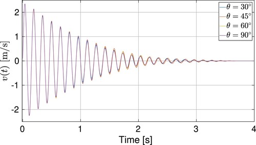
Additionally, several snapshots of the different simulations carried out are shown in Figure 17 at four time instants from the initial stages of the simulation. From the evolution, it can be seen that at the first impact simulations with a measurable meniscus behave similarly, with the expected three pocket shape that is observed in the experiments. As contact angle is increased, it can be appreciated that the thickness of the main central branch increases, and also that the central gas bubble closes more slowly. Conversely, a considerably different behavior is observed when meniscus is not present ($\theta ={90}^{\circ }$). In that case, free surface instabilities develop differently and several thin jets along the surface can be observed.

Figure 17. Time instants for four simulations with different contact angles. First row: t = 0.0s, second $t=0.1\mathrm{s}$, third $t=0.25\mathrm{s}$, fourth $t=0.5\mathrm{s}$. Columns, from left to right: $\theta ={30}^{\circ }$, $\theta ={45}^{\circ }$, $\theta ={60}^{\circ }$, $\theta ={90}^{\circ }$.

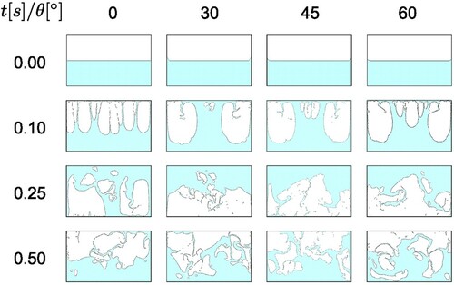
As the simulation evolves further in time, and the second stage is developed, with a highly fragmented free surface observed, and differences between simulations are less obvious.

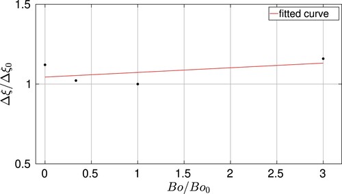
In order to quantify Bond number influence on the overall damping of the experiment, the results obtained for the different simulations are shown in Figure 18, where the reference case used for normalization and designated with a ${}_0$ subindex is the $\theta ={45}^{\circ }$. As can be seen, there is not a big difference between the different cases, being that the highest value obtained for the highest Bond number corresponds to the lowest angle tested ($\theta ={30}^{\circ }$). In any case, the maximum variation in damping is found to be around 15% over the damping corresponding to the reference case.

Figure 18. Damping ratio variation with FSI computations for four different Bo numbers.

4.3.2. Weber number dependence

In order to evaluate the influence of the surface tension during the evolution of the dynamics of the problem, several computational tests have been performed using four additional surface tensions besides the water case. As a consequence, only the non-dimensional Weber number is varied. This kind of study cannot be performed experimentally, because changing the fluid would affect other non-dimensional numbers. In this study the surface tension range covered is $[0.5-2.5]$ times the water surface tension ${\sigma }_0$ and uses a 50% filling level in all cases. The differences in terms of tank velocity and damping ratio are evaluated. 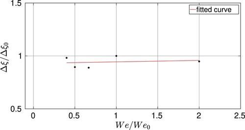In Figures 19 and 20, the computed tank velocity and the damping ratio are represented for the five different surface tension values, where the reference case used for normalization, and designated with a ${}_0$ subindex is the water surface tension case. We observe that the surface tension variations do not substantially affect either the tank velocity or the fluid extra-damping. In conclusion, it can be concluded that the Weber number is not a determinant non-dimensional in these kinds of sloshing experiments.

Figure 19. Comparison of the evolution of the tank velocity when the FSI computation is performed for five different surface tension values.

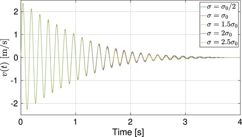
Figure 20. Evolution of the damping ratio added to the system by the fluid using FSI computations for five different We numbers.

4.3.3. Froude number dependence

Different initial amplitudes, or their equivalent initial accelerations, have been used in the simulation in order to evaluate the influence of the Froude number while the rest of the non-dimensional numbers remains constant. In contrast to other non-dimensional number studies, in this case the computational results can be compared to the experiments performed.

In Figure 21, the normalized extra-damping obtained computationally and experimentally is represented as a function of the inverse of the Froude number, where the reference case used for normalization of the vertical axis is designated with a ${}_0$ subindex and corresponds to a = 10g. Despite some quantitative discrepancies, both curves have a good qualitative agreement in terms of describing the Froude dependence. Larger initial accelerations imply larger values of the inverse of the Froude number. 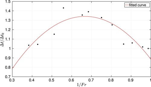We can observe that there is a critical value $1/Fr\approx 0.65$ where the increasing tendency of the extra-damping stops, the system saturates and no longer gives higher damping ratio levels for higher amplitudes. By computing the time-shift between the sloshing force and the tank velocity plotted in Figure 22 we observe that there is a critical Froude number region for which the time-shift is higher, enabling a larger fluid power dissipation and therefore adding a higher damping to the system. However, for higher and lower amplitudes, the time-shift decreases, leading to lower damping ratio levels.

Figure 21. Comparison of the experimental and numerical evolution of the damping ratio added to the system by the fluid using FSI computations for 12 different Fr numbers.

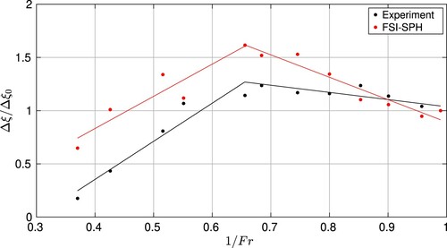
Figure 22. Normalized time-shift between the sloshing force and the tank velocity as a function of the inverse of the Fr number using FSI-SPH computations.

4.3.4. Reynolds number dependence

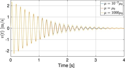
Several values of viscosity have been varied in the simulation in order to evaluate the influence of the Reynolds number, keeping the rest of non-dimensional numbers constant. Similarly to what happens with the surface tension study performed in Section 4.3.2, this kind of study can only be performed computationally, which allows focusing exclusively on the Reynolds number variations. In this study, the dynamic viscosity of the fluid µ is changed from 100 times less than the water viscosity ${\mu }_0$ to 3 orders of magnitude over it. Such a variation includes simulations carried out both at the laminar and the turbulent regimes.

Again, the differences are evaluated in terms of the influence such a change has on the tank motion. In Figure 23, the tank velocity is observed for three different values of viscosity: minimum, reference and maximum viscosity. It can be appreciated that in general, changes remain quite small, being that these are more noticeable at the last stages, when the third regime described in Section 4.1 arises. However, some remarkable properties can be outlined. First, the differences between the minimum and the reference values are quite small, whilst increasing viscosity to the maximum value implicates a greater difference. This may be due to the fact that the minimum and the reference values correspond to the same regime, i.e. the turbulent regime, in contrast to the maximum viscosity value where the Reynolds number is low enough to be considered as a laminar regime. Also, velocity reduction is maximum for the reference case. With a more turbulent case, reduction is lower, but close to the reference value, suggesting that Reynolds number is not particularly relevant in this context where the flow is turbulent. On the contrary, the maximum value of viscosity implies the lower reduction in tank velocity, and hence a lower dissipation is expected.

Figure 23. Velocity of the tank using FSI computations for liquid viscosities ${10}^{-2}$, 1, and 1000 times the dynamic viscosity of water ${\mu }_0$.

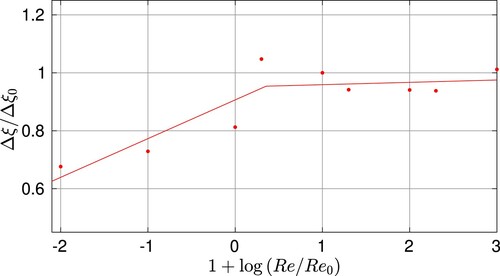
In order to confirm these trends, results are presented in terms of damping in Figure 24, where the reference case used for normalization, and designated with a ${}_0$ subindex, is the water viscosity case. As it is shown there, damping is similar when Reynolds number is relatively high, and at a certain point it starts decreasing when Reynolds number decreases, close to the critical Reynolds number for these kinds of flows. This result confirms that for more viscous fluid damping is lower, and hence that viscosity is not the main parameter related to the damping mechanisms in this vertical sloshing flow.

Figure 24. Evolution of the damping ratio added to the system by the fluid using FSI computations for nine different Re numbers.

4.3.5. Mass ratio dependence

In this section, we are going to present the sloshing results when the sloshing fluid density is changed. Four different densities have been used in the simulations in order to evaluate the influence of the mass ratio keeping the rest of non-dimensional numbers constant. To achieve this goal, the dynamic viscosity and the surface tension have been multiplied by the same factor as the density in order to keep the Reynolds and the Weber number constant. Another important issue is to keep the total mass of the system equal to the one used in the reference water case, this is $m=m_s+m_l=2.582$ kg constant. The mass ratio can be expressed as (24) $r=\frac{m_s}{m_l}=\frac{m-\mathrm{\Delta }m}{m_l}$(24) where $\mathrm{\Delta }m$ is the mass difference in the liquid fluid mass when water is replaced by a different liquid. The importance to keep the total mass of the system constant is related with the necessity to keep both the natural frequency of the system ${\omega }_0$ and the Froude number also constant. In contrast to the previous cases, in this case liquid density changes affect more dimensional numbers than the mass ratio r. Consequently, it is important to change the magnitudes that make all the non-dimensional numbers (Re, We, Fr, Bo) with the exception of the massratio r.

In this study, the density of the fluid ρ is increased 0.5,1, 1.5 and 2 times the water density ${\rho }_0$, the filling level being 50% in all cases. The mass ratio range corresponding to these four cases, including the water case, is $r\in [5.15,23.1]$.

In contrast to the previous cases, important differences in terms of sloshing force and tank velocity are observed. In Figure 25, the tank velocity is monitored for four different densities. We can observe that although there is an irregular alternation of the four different densities in terms of force, the tank velocity is clearly regulated by the density changes, where clearly the larger the fluid density, the larger the damping. In Figure 26, the extra damping is represented as a function of the inverse of the mass ratio, where the reference case used for normalization, and designated with a ${}_0$ subindex, is the water case. The linear trend exhibited by the damping shows that the liquid density is a determinant factor for the sloshing phenomenon. In conclusion, we can state that in this turbulent context, the mass ratio clearly affects the liquid damping during these kinds of sloshing experiments.

Figure 25. Velocity of the tank over time computed with FSI simulations for 0.5, 1,1.5 and 2 times the density of water ${\rho }_0$.

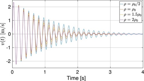
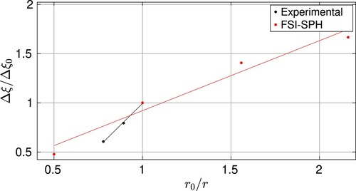
Figure 26. Comparison between experimental and numerical results of the damping added by the fluid as a function of the inverse of the mass ratio r.

4.3.6. Summary of the non-dimensional analysis of the fluid added damping.

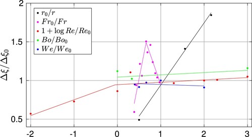
In Sections 4.3.1 and 4.3.2, several results have been presented, varying the contact angle and the surface tension in a range close to the water, where little variations are observed in the damping of the tank velocity. In Section 4.3.3, the initial deformation of the system or its equivalent initial acceleration was varied, the added damping presents a maximum corresponding to an optimum phase shift between the sloshing force and tank velocity. Afterwards, in Section 4.3.4 the liquid viscosity is changed to vary the Reynolds number, and only when the Reynolds number is below a critical threshold $R{e}_c$ (critical Reynolds number), the damping of the tank velocity clearly changes. This critical Reynolds number $R{e}_c$ is orders of magnitude lower than the turbulent ones considered in violent events of the transportation industry, and as consequence little extra-damping variations are expected due to viscosity changes. Finally, in Section 4.3.5 the liquid density is varied, and consequently the mass ratio is changed. In this situation, we observed an important and linear increase of damping variation. All these results are compared in Figure 27. Looking at the global representation of the extra-damping versus the five non-dimensional numbers, we can conclude that in this single phase computational study, the mass ratio is the most relevant non-dimensional number.

Figure 27. Evolution of the added damping by the fluid to the system as a function of the mass ratio, Froude number, Reynolds number, Bond number and Weber number using FSI computations.

In order to have an experimental reference for these results in the case of a fixed Fr number, and according to the different sensitivities with the different non-dimensional numbers, we can simplify expression (21(21) $\mathrm{\Delta }\xi =f(Re,Fr,We,Bo,r)$(21) ) to the approximated version $\mathrm{\Delta }\xi \approx f_{comp}\left(r\right)$. In Figure 26, the extra-damping obtained in the four cases described and computed in Section 4.3.5 and the experimental extra-damping obtained for the four different fluids (water, oil, acetone and glycerine) are both represented as a function of a normalized version of the inverse of the mass ratio. A similar linear trend is observed in both cases. Of course, some differences appear between the computational and the experimental cases. Apart from typical three-dimensional effects and numerical errors, these particular differences can be explained with the following arguments:

• A second gas phase is present in the experiments while the computations are performed with a single phase. As result some non-dimensional numbers such as $\frac{{\rho }_a}{{\rho }_f},\frac{{\mu }_a}{{\mu }_f}$ have been neglected in the SPH computations.

• In the experiments, when the inner liquid is changed, not only the mass ratio r varies, but other non-dimensional numbers such as the Reynolds, the Weber and the Bond numbers also change for the four fluids represented in the experimental results.

5. Conclusion

In this paper, we tried to analyze and study, from both experimental and computational perspectives, a coupled FSI system formed by a vertically guided tank system which contains a fluid initially activated by a violent spring action. The system is a simplified version of the fuel tanks present in the wings of aircraft when gust and turbulence accelerate the wing structure, and sloshing phenomena take place inside the tanks. In order to understand the extra-damping obtained by the sloshing action in the coupled system, a non-dimensional analysis is initially performed in order to find out which are the most relevant numbers in this system. The SPH computational approach allows varying of a single non-dimensional number without affecting the rest, something that is difficult to perform in an experimental setting. The first conclusion is that the coupled FSI system, formed by a forced and damped mass-spring system plus the SPH representation of the fluid, is able to accurately approximate the experimental results in terms of sloshing force and tank dynamics, either in the forced or the FSI cases. For this system, where scaling effects are not considered, and a single geometrical setup is studied, several non-dimensional numbers such as: the Bond, Weber, Froude, Reynolds numbers and the mass ratio have been varied independently. A second important conclusion is that the mass ratio and the Froude numbers have been clearly identified as the most sensitive non-dimensional ones in terms of extra-damping added by the fluid to the system. The extra-damping presents a maximum value when the Froude number is varied due to an optimal time shift between the sloshing force and the tank velocity. The most relevant non-dimensional number is the mass ratio which linearly affects the extra damping action. The importance of the mass ratio, as the most relevant non-dimensional number of the system, has been compared to the experimental results obtained for different fluids, all showing linear tendencies.

As future work, we would like to study deeper into the importance of the phase shifts between the sloshing force and the tank velocity. A second improvement that should be made in the future should come from completing the SPH formulation with the possibility of including a second phase in the simulation. Also, an extension to 3-D would be desirable to check how these effects can modify the trends in the curves obtained. Additionally, including an LES turbulence model to the formulation, adapted from previous works such as Meringolo et al. (2019) might help to clarify aspects linked to the energy dissipation of the system when high Reynolds numbers are involved.

Finally, the size of the tank should be scaled, and the forces and damping ratios should be both computed and measured in order to see if the scaling laws work properly.

Acknowledgments

The research leading to these results was undertaken as part of the SLOWD project, which has received funding from the European Union's Horizon 2020 research and innovation programme under grant agreement No. 815044. Leo M. González acknowledges the financial support from the Spanish Ministry for Science, Innovation and Universities (MCIU) under grant RTI2018-096791-B-C21 Hidrodinámica de elementos de amortiguamiento del movimiento de aerogeneradores flotantes. All the authors would like to thank Mr. Ciaran Stone for his valuable assistance during the preparation of this manuscript.

Disclosure statement

No potential conflict of interest was reported by the author(s).

Additional information

Funding

This work was supported by Horizon 2020 Framework Programme [815044].

References

- Antuono M., Bouscasse B., Colagrossi A., & Lugni C. (2012). Two-dimensional modal method for shallow-water sloshing in rectangular basins. Journal of Fluid Mechanics, 700, 419–440. https://doi.org/https://doi.org/10.1017/jfm.2012.140
- Antuono M., Colagrossi A., & Marrone S. (2012). Numerical diffusive terms in weakly-compressible SPH schemes. Computer Physics Communications, 183(12), 2570–2580. https://doi.org/https://doi.org/10.1016/j.cpc.2012.07.006
- Antuono M., Colagrossi A., Marrone S., & Molteni D. (2010). Free-surface flows solved by means of SPH schemes with numerical diffusive terms. Computer Physics Communications, 181(3), 532–549. https://doi.org/https://doi.org/10.1016/j.cpc.2009.11.002
- Antuono M., Sun P., Marrone S., & Colagrossi A. (2021). The δ-ALE-SPH model: an arbitrary Lagrangian-Eulerian framework for the δ-SPH model with particle shifting technique. Computers & Fluids, 216, 104806. https://doi.org/https://doi.org/10.1016/j.compfluid.2020.104806
- Arndt T.O., & Dreyer M.E. (2008). Damping behavior of sloshing liquid in laterally excited cylindrical propellant vessels. Journal of Spacecraft and Rockets, 45(5), 1085–1088. https://doi.org/https://doi.org/10.2514/1.35019
- Banim R., Lamb R., & Bergeon M. (2006). Smoothed particle hydrodynamics simulation of fuel tank sloshing. In Proceedings 25th international congress of the aeronautical sciences.
- Batchelor J. (1973). Introduction to fluid dynamics [Russian translation]. MIR.
- Bouscasse B., Colagrossi A., Souto-Iglesias A., & Cercos-Pita J. (2014a). Mechanical energy dissipation induced by sloshing and wave breaking in a fully coupled angular motion system. I. Theoretical formulation and numerical investigation. Physics of Fluids, 26(3), 033103. https://doi.org/https://doi.org/10.1063/1.4869233
- Bouscasse B., Colagrossi A., Souto-Iglesias A., & Cercos-Pita J. (2014b). Mechanical energy dissipation induced by sloshing and wave breaking in a fully coupled angular motion system. II. Experimental investigation. Physics of Fluids, 26(3), 033104. https://doi.org/https://doi.org/10.1063/1.4869234
- Bredmose H., Brocchini M., Peregrine D., & Thais L. (2003). Experimental investigation and numerical modelling of steep forced water waves. Journal of Fluid Mechanics, 490, 217–249. https://doi.org/https://doi.org/10.1017/S0022112003005238
- Bulian G., & Cercos-Pita J.L. (2018). Co-simulation of ship motions and sloshing in tanks. Ocean Engineering, 152, 353–376. https://doi.org/https://doi.org/10.1016/j.oceaneng.2018.01.028
- Bulian G., Souto-Iglesias A., Delorme L., & Botia-Vera E. (2010). Smoothed particle hydrodynamics (SPH) simulation of a tuned liquid damper (TLD) with angular motion. Journal of Hydraulic Research, 47, 28–39. https://doi.org/https://doi.org/10.1080/00221686.2010.9641243
- Calderon-Sanchez J., Cercos-Pita J., & Duque D. (2019). A geometric formulation of the Shepard renormalization factor. Computers & Fluids, 183, 16–27. https://doi.org/https://doi.org/10.1016/j.compfluid.2019.02.020
- Cercos-Pita J.L. (2015). AQUAgpusph, a new free 3D SPH solver accelerated with OpenCL. Computer Physics Communications, 192, 295–312. https://doi.org/https://doi.org/10.1016/j.cpc.2015.01.026
- Chiron L., De Leffe M., Oger G., & Le Touzé D. (2019). Fast and accurate SPH modelling of 3-D complex wall boundaries in viscous and non viscous flows. Computer Physics Communications, 234, 93–111. https://doi.org/https://doi.org/10.1016/j.cpc.2018.08.001
- Colagrossi A., Antuono M., & Le Touzé D. (2009). Theoretical considerations on the free-surface role in the smoothed-particle-hydrodynamics model. Physical Review E, 79(5), 1–13. https://doi.org/https://doi.org/10.1103/PhysRevE.79.056701
- Colagrossi A., Delorme L., Colicchio G., Souto-Iglesias A., & Cercós-Pita J. (2008). Reynolds number and shallow depth sloshing. In Proceedings of the 3rd ERCOFTAC SPHERIC Workshop on SPH applications.
- Constantin L., Courcy J.D., Titurus B., Rendall T., & Cooper J.E. (2020). Analysis of damping from vertical sloshing in a SDOF system. Mechanical Systems Signal Processing, 152, 107452. https://doi.org/https://doi.org/10.1016/j.ymssp.2020.107452
- Delorme L., Colagrossi A., Souto-Iglesias A., Zamora-Rodríguez R., & Botía-Vera E. (2009). A set of canonical problems in sloshing, part I: pressure field in forced roll-comparison between experimental results and SPH. Ocean Engineering, 36, 168–178. https://doi.org/https://doi.org/10.1016/j.oceaneng.2008.09.014
- Demirbilek Z. (1983a). Energy dissipation in sloshing waves in a rolling rectangular tank – I. Mathematical theory. Ocean Engineering, 10(5), 347–358. https://doi.org/https://doi.org/10.1016/0029-8018(83)90004-5. http://www.sciencedirect.com/science/article/pii/0029801883900069
- Demirbilek Z. (1983b). Energy dissipation in sloshing waves in a rolling rectangular tank – II. Solution method and analysis of numerical technique. Ocean Engineering, 10(5), 359–374. https://doi.org/https://doi.org/10.1016/0029-8018(83)90005-7. http://www.sciencedirect.com/science/article/pii/0029801883900069
- Demirbilek Z. (1983c). Energy dissipation in sloshing waves in a rolling rectangular tank – III. Results and applications. Ocean Engineering, 10(5), 375–382. https://doi.org/https://doi.org/10.1016/0029-8018(83)90006-9. http://www.sciencedirect.com/science/article/pii/0029801883900069
- Di Mascio A., Antuono M., Colagrossi A., & Marrone S. (2017). Smoothed particle hydrodynamics method from a large eddy simulation perspective. Physics of Fluids, 29(3), 035102. https://doi.org/https://doi.org/10.1063/1.4978274
- Faltinsen O.M., & Timokha A.N. (2009). Sloshing (Vol. 577). Cambridge University Press.
- Farhadi A., Emdad H., & Rad E.G. (2016). Incompressible SPH simulation of landslide impulse-generated water waves. Natural Hazards, 82(3), 1779–1802. https://doi.org/https://doi.org/10.1007/s11069-016-2270-8
- Frandsen J. (2005). Numerical predictions of tuned liquid tank structural systems. Journal of Fluids and Structures, 20(3), 309–329. https://doi.org/https://doi.org/10.1016/j.jfluidstructs.2004.10.003
- Gambioli F., & Malan A. (2017). Fuel loads in large civil airplanes. In International forum on aeroelasticity and structural dynamics IFASD.
- Gimenez J.M., & González L.M. (2015). An extended validation of the last generation of particle finite element method for free surface flows. Journal of Computational Physics, 284, 186–205. https://doi.org/https://doi.org/10.1016/j.jcp.2014.12.025
- Gingold R.A., & Monaghan J.J. (1977). Smoothed particle hydrodynamics: theory and application to non-spherical stars. Monthly Notices of the Royal Astronomical Society, 181(3), 375–389. https://doi.org/https://doi.org/10.1093/mnras/181.3.375
- Gómez-Goñi J., Garrido-Mendoza C.A., Cercós J.L., & González L. (2013). Two phase analysis of sloshing in a rectangular container with Volume of Fluid (VOF) methods. Ocean Engineering, 73, 208–212. https://doi.org/https://doi.org/10.1016/j.oceaneng.2013.07.005
- Ibrahim R.A. (2005). Liquid sloshing dynamics: theory and applications. Cambridge University Press.
- Li J., Hamamoto Y., Liu Y., & Zhang X. (2014). Sloshing impact simulation with material point method and its experimental validations. Computers & Fluids, 103, 86–99. https://doi.org/https://doi.org/10.1016/j.compfluid.2014.07.025
- Lind S.J., Xu R., Stansby P.K., & Rogers B.D. (2012). Incompressible smoothed particle hydrodynamics for free-surface flows: a generalised diffusion-based algorithm for stability and validations for impulsive flows and propagating waves. Journal of Computational Physics, 231(4), 1499–1523. https://doi.org/https://doi.org/10.1016/j.jcp.2011.10.027
- Lucy L.B. (1977). A numerical approach to the testing of the fission hypothesis. The Astronomical Journal, 82, 1013–1024. https://doi.org/https://doi.org/10.1086/112164
- Marrone S., Colagrossi A., Le Touzé D., & Graziani G. (2010). Fast free-surface detection and level-set function definition in SPH solvers. Journal of Computational Physics, 229(10), 3652–3663. https://doi.org/https://doi.org/10.1016/j.jcp.2010.01.019
- Marrone S., Colagrossi A., Mascio A.D., & Touzé D.L. (2015). Prediction of energy losses in water impacts using incompressible and weakly compressible models. Journal of Fluids and Structures, 54, 802–822. https://doi.org/https://doi.org/10.1016/j.jfluidstructs.2015.01.014
- Martinez-Carrascal J., & Gonzalez-Gutierrez L.M. (2020). Experimental study of the liquid damping effects on a SDOF vertical sloshing tank. Journal of Fluids and Structures, 100, 103172. https://doi.org/https://doi.org/10.1016/j.jfluidstructs.2020.103172
- Meringolo D.D., Marrone S., Colagrossi A., & Liu Y. (2019). A dynamic δ-SPH model: how to get rid of diffusive parameter tuning A dynamic δ-SPH model: how to get rid of diffusive parameter tuning. Computers & Fluids, 179, 334–355. https://doi.org/https://doi.org/10.1016/j.compfluid.2018.11.012
- Moirod N., Diebold L., Baudin E., & Gazzola T. (2011). Experimental and numerical investigations of internal global forces for violent irregular excitations in LNGC prismatic tanks. In Proceedings of the 21st international offshore and polar engineering conference.
- Monaghan J.J. (1994). Simulating free surface flows with SPH. Journal of Computational Physics, 110(2), 399–406. https://doi.org/https://doi.org/10.1006/jcph.1994.1034
- Monaghan J.J. (2000). SPH without a tensile instability. Journal of Computational Physics, 159(2), 290–311. https://doi.org/https://doi.org/10.1006/jcph.2000.6439
- Morris J.P. (2000). Simulating surface tension with smoothed particle hydrodynamics. International Journal for Numerical Methods in Fluids, 33(3), 333–353. https://doi.org/https://doi.org/10.1002/(ISSN)1097-0363
- Randles P., & Libersky L. (1996). Smoothed particle hydrodynamics: some recent improvements and applications. Computer Methods in Applied Mechanics and Engineering, 139, 375–408. https://doi.org/https://doi.org/10.1016/S0045-7825(96)01090-0
- Rogers J., & Szymczak W. (1997). Computations of violent surface motions: comparisons with theory and experiments. Philosophical Transactions: Mathematical, Physical and Engineering Sciences, 355, 649–663. https://doi.org/https://doi.org/10.1098/rsta.1997.0031
- Salih S.Q., Aldlemy M.S., Rasani M.R., Ariffin A.K., Ya T.M.Y.S.T., Al-Ansari N., Yaseen Z.M., & Chau K.W. (2019). Thin and sharp edges bodies-fluid interaction simulation using cut-cell immersed boundary method. Engineering Applications of Computational Fluid Mechanics, 13(1), 860–877. https://doi.org/https://doi.org/10.1080/19942060.2019.1652209
- Serván-Camas B., Cercós-Pita J., Colom-Cobb J., García-Espinosa J., & Souto-Iglesias A. (2016). Time domain simulation of coupled sloshing–seakeeping problems by SPH–FEM coupling. Ocean Engineering, 123, 383–396. https://doi.org/https://doi.org/10.1016/j.oceaneng.2016.07.003
- Souto-Iglesias A., Delorme L., Pérez-Rojas L., & Abril-Pérez S. (2006). Liquid moment amplitude assessment in sloshing type problems with smooth particle hydrodynamics. Ocean Engineering, 33, 1462–1484. https://doi.org/https://doi.org/10.1016/j.oceaneng.2005.10.011
- Souto-Iglesias A., Pérez-Rojas L., & Zamora-Rodríguez R. (2004). Simulation of anti-roll tanks and sloshing type problems with smoothed particle hydrodynamics. Ocean Engineering, 31, 1169–1192. https://doi.org/https://doi.org/10.1016/j.oceaneng.2003.09.002
- Stasch J., Avci B., & Wriggers P. (2016). Numerical simulation of fluid-structure interaction problems by a coupled SPH-FEM approach. Proceedings in Applied Mathematics and Mechanics, 16(1), 491–492. https://doi.org/https://doi.org/10.1002/pamm.201610234
- Sun P., Colagrossi A., Marrone S., Antuono M., & Zhang A. (2018). Multi-resolution delta-plus-SPH with tensile instability control: towards high Reynolds number flows. Computer Physics Communications, 224, 63–80. https://doi.org/https://doi.org/10.1016/j.cpc.2017.11.016
- Sun P., Colagrossi A., Marrone S., Antuono M., & Zhang A.M. (2019). A consistent approach to particle shifting in the δ-Plus-SPH model A consistent approach to particle shifting in the δ-plus-SPH model. Computer Methods in Applied Mechanics and Engineering, 348, 912–934. https://doi.org/https://doi.org/10.1016/j.cma.2019.01.045
- Sun L., & Fujino Y. (1994). A semi-analytical model for tuned liquid dampers (TLD) with wave breaking. Journal of Fluids and Structures, 8, 471–488. https://doi.org/https://doi.org/10.1006/jfls.1994.1023
- Sykes B.S., Malan A.G., & Gambioli F. (2018). Novel nonlinear fuel slosh surrogate reduced-order model for aircraft loads prediction. Journal of Aircraft, 55(3), 1004–1013. https://doi.org/https://doi.org/10.2514/1.C033860
- Tait M. (2008). Modelling and preliminary design of a structure-TLD system. Engineering Structures, 30(10), 2644–2655. https://doi.org/https://doi.org/10.1016/j.engstruct.2008.02.017
- Titurus B., Cooper J.E., Saltari F., Mastroddi F., & Gambioli F. (2019). Analysis of a sloshing beam experiment. In International forum aeroelasticity and structural dynamics.
- Yu J.K., Wakahara T., & Reed D.A. (1999). A non-linear numerical model of the tuned liquid damper. Earthquake Engineering & Structural Dynamics, 28(6), 671–686. https://doi.org/https://doi.org/10.1002/(SICI)1096-9845(199906)28:6<671::AID-EQE835>3.0.CO;2-X