Adjoint-based shape optimization for the minimization of flow-induced hemolysis in biomedical applications

Abstract

This paper reports on the derivation and implementation of a shape optimization procedure for the minimization of hemolysis induction in blood flows through biomedical devices.Despite the significant progress in relevant experimental studies, the ever-growing advances in computational science have made computational fluid dynamics an indispensable tool for the design of biomedical devices. However, even the latter can lead to a restrictive cost when the model requires an extensive number of computational elements or when the simulation needs to be overly repeated. This work aims at the formulation of a continuous adjoint complement to a power-law hemolysis prediction model dedicated to efficiently identifying the shape sensitivity to hemolysis. The proposed approach can accompany any gradient-based optimization method at the cost of approximately one additional flow solution per shape update. The approach is verified against analytical solutions of a benchmark problem and computed sensitivity derivatives are validated by a finite differences study on a generic 2D stenosed geometry. The included application addresses a 3D ducted geometry which features typical characteristics of blood-carrying devices. An optimized shape, leading to a potential improvement up to 22%, is identified. It is shown that the improvement persists for different hemolysis-evaluation parameters.

Keywords:

• Computational fluid dynamics(CFD)
• adjoint-based shape optimization
• biomedical design
• hemolysis minimization

1. Introduction

The ever-growing advances in medicine, engineering and material science have led to the development of biomedical devices, such as blood pumps, which allow long-term patient care and significantly improve quality of life. Despite all the advances, a critical task for the design and development of such devices (Thamsen et al., 2015; Yu et al., 2016) is still the minimization of shear-induced blood damage (i.e. hemolysis) to guarantee good bio-compatibility.

In the context of this work, hemolysis refers to the mechanical damage of red blood cells due to excessively high stress induced by peculiarities of the blood flow. It can lead to hemoglobinemia, which plays a significant role in the pathogenesis of sepsis, and to increased risk of infection due to its inhibitory effects on the innate immune system (Effenberger-Neidnicht & Hartmann, 2018). Hemolysis induction is encountered in many biomedical devices, where large velocity gradients are found (De Somer et al., 1996), as well as in vivo conditions when vessels delivering blood are kinked or stenosed (Goubergrits et al., 2018). The shape of the respective artificial devices or vessels is believed to play a crucial part in the induction of blood damage due to its decisive fluid dynamic role. The extent to which experimental studies can provide novel biomedical designs is restricted by the inevitable limitations of blood-treating processes. On the other hand, the ever-growing advances in computational science have made computational fluid dynamics (CFD) simulations an indispensable tool for the study of real case applications (Ghalandari et al., 2019; Salih et al., 2019). At the same time, however, computational optimization methods can also lead to restrictive costs when simulations of 3D models need to be overly repeated or the design needs a certain degree of detail, leading to large computational models. This work targets the development of a computationally efficient shape optimization framework so that to viably assist the design of next-generation biomedical machinery.

The success of a numerical optimization process partially depends on the accuracy of the hemolysis-prediction model. While the study of shear-induced hemolysis has been of interest for many experimental, in vitro conditions for quite some time (Giersiepen et al., 1990; Heuser & Opitz, 1980; Zhang et al., 2011), it is also becoming increasingly important in silico conditions (Stewart et al., 2012; Yu et al., 2017). CFD offer the possibility to predict blood damage in a purely numerical manner and employ the damage prediction model as a cost function in an optimization framework. A variety of such damage prediction models have been proposed (Yu et al., 2017). Most of them relate hemolysis with the magnitude of the shear stress and an exposure period using a variation of a power-law formulation, initially suggested by Giersiepen et al. (1990).

Despite the remarkable progress, a numerical model able to satisfactorily predict blood damage in a variety of flows has not yet been established (Goubergrits et al., 2018). The present paper does not aim to advocate the merits of a specific hemolysis evaluation or hemolysis prediction model, but is mainly concerned with the adaptation and integration of a classical model into an adjoint shape optimization framework. Employing an Eulerian hemolysis-prediction model alongside a common CFD solver, we formulate a Partial-Differential-Equation (PDE) constrained optimization problem, which targets to minimize flow-induced hemolysis by improving the shape. In the context of this paper, hemolysis will be referred to as objective while the shape as control. In CFD-based optimization, multiple ways, ranging from stochastic (Bäck, 1996; Michalewicz, 1994) to deterministic (Bertsekas, 1996; Thévenin & Janiga, 2008) optimization methods, could be followed. The present research is concerned with the efficient computation of the derivative of the objective with respect to (w.r.t) the control. The aforementioned derivative is subsequently used by a deterministic gradient-based steepest descent method, which drives the controlled shape towards an improved state. To that extent, the continuous adjoint method is studied. The adjoint method has been, increasingly, receiving attention in terms of CFD-based optimization (Heners et al., 2018; Papadimitriou & Giannakoglou, 2007; Papoutsis-Kiachagias & Giannakoglou, 2016; Papoutsis-Kiachagias et al., 2019; Stück & Rung, 2013) since the pioneering works of Pironneau (1974) and Jameson (1988), due to its superior computational efficiency. In specific, the attractiveness of the method lies on the fact that the computation of the derivative is independent from the size of the control. For further details on the merits and drawbacks of the adjoint approach, the interested reader is referred to Giles and Pierce (2000) and Martins and Hwang (2013).

The remainder of this paper is organized as follows: Section 2 presents the mathematical model of the primal and adjoint problem. The same section also reports on the employed numerical procedure and utilized boundary conditions (BCs). In Section 3, a benchmark case is studied to verify the code reliability. Moreover, the accuracy of the computed sensitivity derivative is assessed in the context of a Finite Differences (FD) study. Subsequently, in Section 4, the model is applied on a 3D geometry. Results for a full shape optimization process are presented and their dependency on parameters of the nonlinear hemolysis evaluation model is discussed. The paper closes with conclusions and outlines further research in Section 5.

Within this publication, Einstein's summation convention is used for repeated lower-case Latin subscripts. Vectors and tensors are defined with reference to Cartesian coordinates.

2. Mathematical model

This section is dedicated to the formulation of the primal (physical) and adjoint (dual) problem. The coupling of the hemolysis-prediction model with the primal flow equations is discussed. A presentation of the newly developed adjoint model then follows with detailed discussions on adjoint-hemolysis specific points of interest.

2.1. Primal flow

Throughout this paper, blood is treated exclusively as an incompressible, Newtonian fluid. While the assumption of Newtonian properties has been shown to fall short of modelling blood flows with relatively low shear rates, it is generally widely used (Stewart et al., 2012). Our work is, thus, restricted to a Newtonian viscosity description to simplify the derivation of the adjoint model. Furthermore, for the application presented in this work, a maximum Re = 500 is assumed and so our state is considered laminar but also steady. The blood flow in a domain (Ω) follows from the Navier–Stokes (NS) equations for the conservation of volume and momentum, viz. (1) $\begin{array}{rl}{R}^p& =-\frac{\mathrm{\partial }{u}_j}{\mathrm{\partial }{x}_j}=0,\end{array}$(1) (2) $\begin{array}{rl}{R}_i^u& =\rho u_j\frac{\mathrm{\partial }{u}_i}{\mathrm{\partial }{x}_j}-\frac{\mathrm{\partial }}{\mathrm{\partial }{x}_j}\left[2\mu S_{ij}-p{\delta }_{ij}\right]=0.\end{array}$(2) Here $u_i$, p, $S_{ij}=0.5(\mathrm{\partial }{u}_i/\mathrm{\partial }{x}_j+\mathrm{\partial }{u}_j/\mathrm{\partial }{x}_i)$, ${\delta }_{ij}$, ρ and μ refer to the components of the fluid velocity vector, static pressure, components of the strain-rate tensor, Kronecker delta components as well as the fluid density and dynamic viscosity, respectively.

In the framework of CFD-based hemolysis analysis, a typical approach is to utilize a prediction or evaluation model in a one-way coupling with the CFD solver (Yu et al., 2017). This implies that the hemolysis model receives information from the NS Equations (1(1) $\begin{array}{rl}{R}^p& =-\frac{\mathrm{\partial }{u}_j}{\mathrm{\partial }{x}_j}=0,\end{array}$(1) ) and (2(2) $\begin{array}{rl}{R}_i^u& =\rho u_j\frac{\mathrm{\partial }{u}_i}{\mathrm{\partial }{x}_j}-\frac{\mathrm{\partial }}{\mathrm{\partial }{x}_j}\left[2\mu S_{ij}-p{\delta }_{ij}\right]=0.\end{array}$(2) ) with no retro-action on the employed fluid properties ($\rho ,\mu$). The hemolysis prediction model considered in this study originates from the power-law equation, first introduced by Giersiepen et al. (1990), and reads (3) $H(\overline{\tau },t)=C{\overline{\tau }}^{\alpha }{t}^{\text{β}}.$(3) The hemolysis index H denotes a measure for the released hemoglobin to the total hemoglobin within the red blood cell. It is governed by a scalar stress representation $\overline{\tau }$ and an exposure time t, which represents the duration on which the red blood cell is exposed to the stress. The remaining constants (C, α, β) are introduced to fit experimental data. Table 1 summarizes the parameter sets utilized in this study. The second invariant of the stress tensor ${\tau }_{ij}=2\mu S_{ij}$ is frequently used to determine the scalar stress representation $\overline{\tau }$ in combination with a user-specific positive integer parameter k. In this work, k = 1 and k = 2 are solely considered as it is found that these values are sufficient to represent the physics of the presented applications in comparison with experimental values or analytical solutions. (4) $\overline{\tau }=\sqrt{-k{I}_{{\tau }_2}}\mathrm{w}\mathrm{i}\mathrm{t}\mathrm{h}{I}_{{\tau }_2}=\frac{1}{2}\left[\left(tr({\tau }_{ij}{)}^2-tr({\tau }_{ij}^2)\right)\right].$(4) Due to $tr\left({\tau }_{ij}\right)=tr\left(2\mu S_{ij}\right)\sim \mathrm{\partial }{u}_i/\mathrm{\partial }{x}_i$, the first contribution to $I_{{\tau }_2}$ in (4(4) $\overline{\tau }=\sqrt{-k{I}_{{\tau }_2}}\mathrm{w}\mathrm{i}\mathrm{t}\mathrm{h}{I}_{{\tau }_2}=\frac{1}{2}\left[\left(tr({\tau }_{ij}{)}^2-tr({\tau }_{ij}^2)\right)\right].$(4) ) vanishes for incompressible Newtonian fluids, which yields (5) $\overline{\tau }={\left(2k{\mu }^2{S}_{ij}{S}_{ij}\right)}^{\frac{1}{2}}:={{\tau }^{\ast }}^{\frac{1}{2}}.$(5) To incorporate Equation (3(3) $H(\overline{\tau },t)=C{\overline{\tau }}^{\alpha }{t}^{\text{β}}.$(3) ) into an adjoint optimization framework, a PDE-based hemolysis prediction is advantageous. To this end, a linearization strategy is used (Garon & Farinas, 2004) for (3(3) $H(\overline{\tau },t)=C{\overline{\tau }}^{\alpha }{t}^{\text{β}}.$(3) ), i.e. (6) $H^{\frac{1}{\text{β}}}=\left(C^{\frac{1}{\text{β}}}{\overline{\tau }}^{\frac{\alpha }{\text{β}}}\right)t.$(6) Substituting $H_L=H^{\frac{1}{\text{β}}}$, the sought material derivative expression follows from (6(6) $H^{\frac{1}{\text{β}}}=\left(C^{\frac{1}{\text{β}}}{\overline{\tau }}^{\frac{\alpha }{\text{β}}}\right)t.$(6) ) (7) $\rho \frac{\mathrm{\partial }{H}_L}{\mathrm{\partial }t}+\rho u_j\frac{\mathrm{\partial }{H}_L}{\mathrm{\partial }{x}_j}=\rho C^{\frac{1}{\text{β}}}{\overline{\tau }}^{\frac{\alpha }{\text{β}}}.$(7) Assuming steady state, a modification of the residual form of (7(7) $\rho \frac{\mathrm{\partial }{H}_L}{\mathrm{\partial }t}+\rho u_j\frac{\mathrm{\partial }{H}_L}{\mathrm{\partial }{x}_j}=\rho C^{\frac{1}{\text{β}}}{\overline{\tau }}^{\frac{\alpha }{\text{β}}}.$(7) ) reads (8) $R^H=\rho u_j\frac{\mathrm{\partial }{H}_L}{\mathrm{\partial }{x}_j}-\rho C^{\frac{1}{\text{β}}}{\overline{\tau }}^{\frac{\alpha }{\text{β}}}(1-H_L)=0\mathrm{i}\mathrm{n}\mathrm{\Omega }.$(8) Note that (8(8) $R^H=\rho u_j\frac{\mathrm{\partial }{H}_L}{\mathrm{\partial }{x}_j}-\rho C^{\frac{1}{\text{β}}}{\overline{\tau }}^{\frac{\alpha }{\text{β}}}(1-H_L)=0\mathrm{i}\mathrm{n}\mathrm{\Omega }.$(8) ) is enhanced by $(1-H_L)$ to ensure $H_L<1$. Equation (8(8) $R^H=\rho u_j\frac{\mathrm{\partial }{H}_L}{\mathrm{\partial }{x}_j}-\rho C^{\frac{1}{\text{β}}}{\overline{\tau }}^{\frac{\alpha }{\text{β}}}(1-H_L)=0\mathrm{i}\mathrm{n}\mathrm{\Omega }.$(8) ) will be referred to as (primal) hemolysis equation throughout this paper and serves to formulate the objective functional of the optimization. The merits of expression (8(8) $R^H=\rho u_j\frac{\mathrm{\partial }{H}_L}{\mathrm{\partial }{x}_j}-\rho C^{\frac{1}{\text{β}}}{\overline{\tau }}^{\frac{\alpha }{\text{β}}}(1-H_L)=0\mathrm{i}\mathrm{n}\mathrm{\Omega }.$(8) ) refer to its straightforward derivation from the original power-law formulation (3(3) $H(\overline{\tau },t)=C{\overline{\tau }}^{\alpha }{t}^{\text{β}}.$(3) ) and its suitability for showcasing the adjoint method in the context of blood damage. While it is true that hemolysis does not occur for small values of $\overline{\tau }<{\overline{\tau }}_{\mathrm{t}\mathrm{h}}$, where ${\overline{\tau }}_{\mathrm{t}\mathrm{h}}$ corresponds to some threshold value (which might also be related to the exposure time), this aspect is deliberately ignored in the present effort. Furthermore, the footing of the hemolysis model assumes a homogeneous stress representation. Even though this is a strong assumption for most practical applications, the predictions have been shown to be sufficiently reliable when relatively comparing different geometries (Taskin et al., 2012). Nevertheless, the hemolysis results presented in this work enable a qualitative comparison between initial and optimized geometry and should be regarded as such rather than quantitatively.

Table 1. Parameter sets of Equation (3(3) $H(\overline{\tau },t)=C{\overline{\tau }}^{\alpha }{t}^{\text{β}}.$(3) ). The notation corresponds to the initials of the investigators that performed the experiments (GW (Giersiepen et al., 1990), HO (Heuser & Opitz, 1980), ZT (Zhang et al., 2011)). The final two columns correspond to the type of blood that was used and to the maximum stress that was applied during the experiments.

Notation	Values $(C,\alpha ,\text{β})$	Type of Blood	Max. Stress (Pa)
GW	$(3.6\cdot {10}^{-7}$, 2.416, $0.785)$	Human	255
HO	$(1.8\cdot {10}^{-8}$, 1.991, $0.765)$	Porcine	600
ZT	$(1.2\cdot {10}^{-7}$, 1.992, $0.661)$	Ovine	320

Equation (8(8) $R^H=\rho u_j\frac{\mathrm{\partial }{H}_L}{\mathrm{\partial }{x}_j}-\rho C^{\frac{1}{\text{β}}}{\overline{\tau }}^{\frac{\alpha }{\text{β}}}(1-H_L)=0\mathrm{i}\mathrm{n}\mathrm{\Omega }.$(8) ) serves for the formulation of an adjoint complement in Section 2.2.1. Furthermore, the optimization requires a scalar objective functional. An integral index signifying the level of flow-induced hemolysis can be computed from the domain integral $\int {\mathrm{\nabla }}_j\left(\rho u_j{H}_L\right)\mathrm{d}\mathrm{\Omega }$, or a corresponding boundary integral. Assuming zero inflow fluxes of $H_L$, no-slip velocity on the walls and solenoidal flow fields, only the outlet fluxes remain, which are usually normalized by the respective mass flux (9) $H_{index}=\frac{{\int }_{{\mathrm{\Gamma }}_{\mathrm{o}\mathrm{u}\mathrm{t}}}H\rho u_j{n}_j\mathrm{d}\mathrm{\Gamma }}{{\int }_{{\mathrm{\Gamma }}_{\mathrm{o}\mathrm{u}\mathrm{t}}}\rho u_j{n}_j\mathrm{d}\mathrm{\Gamma }}=\frac{{\int }_{{\mathrm{\Gamma }}_{\mathrm{o}\mathrm{u}\mathrm{t}}}{H}_L^{\text{β}}\rho u_j{n}_j\mathrm{d}\mathrm{\Gamma }}{{\int }_{{\mathrm{\Gamma }}_{\mathrm{o}\mathrm{u}\mathrm{t}}}\rho u_j{n}_j\mathrm{d}\mathrm{\Gamma }}.$(9) Note that the denominator of Equation (9(9) $H_{index}=\frac{{\int }_{{\mathrm{\Gamma }}_{\mathrm{o}\mathrm{u}\mathrm{t}}}H\rho u_j{n}_j\mathrm{d}\mathrm{\Gamma }}{{\int }_{{\mathrm{\Gamma }}_{\mathrm{o}\mathrm{u}\mathrm{t}}}\rho u_j{n}_j\mathrm{d}\mathrm{\Gamma }}=\frac{{\int }_{{\mathrm{\Gamma }}_{\mathrm{o}\mathrm{u}\mathrm{t}}}{H}_L^{\text{β}}\rho u_j{n}_j\mathrm{d}\mathrm{\Gamma }}{{\int }_{{\mathrm{\Gamma }}_{\mathrm{o}\mathrm{u}\mathrm{t}}}\rho u_j{n}_j\mathrm{d}\mathrm{\Gamma }}.$(9) ) is constant in steady flows of incompressible fluids. Hence, the numerator of (9(9) $H_{index}=\frac{{\int }_{{\mathrm{\Gamma }}_{\mathrm{o}\mathrm{u}\mathrm{t}}}H\rho u_j{n}_j\mathrm{d}\mathrm{\Gamma }}{{\int }_{{\mathrm{\Gamma }}_{\mathrm{o}\mathrm{u}\mathrm{t}}}\rho u_j{n}_j\mathrm{d}\mathrm{\Gamma }}=\frac{{\int }_{{\mathrm{\Gamma }}_{\mathrm{o}\mathrm{u}\mathrm{t}}}{H}_L^{\text{β}}\rho u_j{n}_j\mathrm{d}\mathrm{\Gamma }}{{\int }_{{\mathrm{\Gamma }}_{\mathrm{o}\mathrm{u}\mathrm{t}}}\rho u_j{n}_j\mathrm{d}\mathrm{\Gamma }}.$(9) ) is considered as an appropriate objective or cost-functional in this work.

2.2. Adjoint method

This subsection outlines the formulation of the adjoint problem at hand which is initially expressed as an optimization problem constrained by a set of PDE, namely $R(y,c)=0$, viz. (10) $\underset{c\in C_{\mathrm{a}\mathrm{d}}}{min}J(y,c)\mathrm{s}.\mathrm{t}.R(y,c)=0.$(10) Here J is the objective or cost functional, y is the vector of primal state variables, which consists of p, $u_i$ and $H_L$, and c is the control parameter which we need to find in the set of admissible states $C_{\mathrm{a}\mathrm{d}}$. In this study, c refers to the shape of the structure in which blood flows. It is thus a subset of $\mathrm{\partial }\mathrm{\Omega }$ or Γ -the latter notation is preferred throughout this paper- and can be further restricted by considering only specific sections of the structure, namely ${\mathrm{\Gamma }}_D\subset \mathrm{\Gamma }$, where the index D denotes design.

Based on (9(9) $H_{index}=\frac{{\int }_{{\mathrm{\Gamma }}_{\mathrm{o}\mathrm{u}\mathrm{t}}}H\rho u_j{n}_j\mathrm{d}\mathrm{\Gamma }}{{\int }_{{\mathrm{\Gamma }}_{\mathrm{o}\mathrm{u}\mathrm{t}}}\rho u_j{n}_j\mathrm{d}\mathrm{\Gamma }}=\frac{{\int }_{{\mathrm{\Gamma }}_{\mathrm{o}\mathrm{u}\mathrm{t}}}{H}_L^{\text{β}}\rho u_j{n}_j\mathrm{d}\mathrm{\Gamma }}{{\int }_{{\mathrm{\Gamma }}_{\mathrm{o}\mathrm{u}\mathrm{t}}}\rho u_j{n}_j\mathrm{d}\mathrm{\Gamma }}.$(9) ) the objective functional under investigation can be written as (11) $J={\int }_{{\mathrm{\Gamma }}_{\mathrm{o}\mathrm{u}\mathrm{t}}}{H}_L^{\text{β}}\rho u_i{n}_i\mathrm{d}\mathrm{\Gamma }={\int }_{{\mathrm{\Gamma }}_{\mathrm{o}\mathrm{u}\mathrm{t}}}{j}_{\mathrm{\Gamma }}\mathrm{d}\mathrm{\Gamma },$(11) while the set of PDE, $R(y,c)=0$, consists of Equations (1(1) $\begin{array}{rl}{R}^p& =-\frac{\mathrm{\partial }{u}_j}{\mathrm{\partial }{x}_j}=0,\end{array}$(1) ), (2(2) $\begin{array}{rl}{R}_i^u& =\rho u_j\frac{\mathrm{\partial }{u}_i}{\mathrm{\partial }{x}_j}-\frac{\mathrm{\partial }}{\mathrm{\partial }{x}_j}\left[2\mu S_{ij}-p{\delta }_{ij}\right]=0.\end{array}$(2) ) and (8(8) $R^H=\rho u_j\frac{\mathrm{\partial }{H}_L}{\mathrm{\partial }{x}_j}-\rho C^{\frac{1}{\text{β}}}{\overline{\tau }}^{\frac{\alpha }{\text{β}}}(1-H_L)=0\mathrm{i}\mathrm{n}\mathrm{\Omega }.$(8) ). Having formulated the optimization problem as a constrained problem in Equations (10(10) $\underset{c\in C_{\mathrm{a}\mathrm{d}}}{min}J(y,c)\mathrm{s}.\mathrm{t}.R(y,c)=0.$(10) ), the Lagrange principle to eliminate the constraints by employing appropriate Lagrange multipliers is utilized (Soto & Löhner, 2004). In this context, a continuous Lagrange functional is defined as (12) $\mathcal{L}:=J+{\int }_{\mathrm{\Omega }}\left[\hat{p}{R}^p+{\hat{u}}_i{R}_i^u+\hat{h}{R}^H\right]\mathrm{d}\mathrm{\Omega },$(12) where $\hat{p}$, ${\hat{u}}_i$ and $\hat{h}$ are Lagrange multipliers that are referred to as adjoint pressure, components of the adjoint velocity vector and adjoint hemolysis, respectively. Their dimensions $\left[{\hat{u}}_{\mathrm{i}}\right]=\left[J\right]/\left(\right[R_{\mathrm{i}}^u\left]m^3\right)$, $\left[\hat{p}\right]=\left[J\right]/\left(\right[R^p\left]m^3\right)$ and $\left[\hat{h}\right]=\left[J\right]/\left(\right[R^H\left]m^3\right)$ depend on the underlying cost functional, where $\left[J\right]=\left(\right[j_{\mathrm{\Gamma }}\left]m^2\right)$ represents the units of the integral boundary-based objective. Since, from a physical point of view, equations $R^p$, $R_i^u$ and $R^H$ are required to be zero, it is apparent that $\mathcal{L}$ is equal to J. The optimization problem (10(10) $\underset{c\in C_{\mathrm{a}\mathrm{d}}}{min}J(y,c)\mathrm{s}.\mathrm{t}.R(y,c)=0.$(10) ) is, thus, equivalent to $min\mathcal{L}(\hat{y},y,c)$, where $\hat{y}$ is the vector of adjoint variables and y is no longer constrained. For a minimum of (12(12) $\mathcal{L}:=J+{\int }_{\mathrm{\Omega }}\left[\hat{p}{R}^p+{\hat{u}}_i{R}_i^u+\hat{h}{R}^H\right]\mathrm{d}\mathrm{\Omega },$(12) ) the total variation $\delta \mathcal{L}$ vanishes (13) $\delta \mathcal{L}=\underset{\mathrm{F}\mathrm{D}1}{\underbrace{{\delta }_{\hat{y}}\mathcal{L}\cdot \delta \hat{y}}}+\underset{\mathrm{F}\mathrm{D}2}{\underbrace{{\delta }_y\mathcal{L}\cdot \delta y}}+\underset{\mathrm{F}\mathrm{D}3}{\underbrace{{\delta }_c\mathcal{L}\cdot \delta c}}=0.$(13) The terms FD1, FD2 and FD3 denote the directional derivative of the Lagrangian in the direction of adjoint ($\delta \hat{y}$) and primal ($\delta y$) state as well as the control ($\delta c$), respectively. They can be computed by utilising the functional derivative into the respective direction. FD1 leads to the known set of primal equations that need to be satisfied for every control state. FD2 yields the accompanying adjoint equations. Finally, FD3 gives rise to a sensitivity derivative that offers information of the objective w.r.t. the control. Equation (13(13) $\delta \mathcal{L}=\underset{\mathrm{F}\mathrm{D}1}{\underbrace{{\delta }_{\hat{y}}\mathcal{L}\cdot \delta \hat{y}}}+\underset{\mathrm{F}\mathrm{D}2}{\underbrace{{\delta }_y\mathcal{L}\cdot \delta y}}+\underset{\mathrm{F}\mathrm{D}3}{\underbrace{{\delta }_c\mathcal{L}\cdot \delta c}}=0.$(13) ) is only satisfied when a global or local minimum is reached. Hence, the following three optimality conditions are obtained for vanishing FD2 (14) $\begin{array}{rl}& {\delta }_p\mathcal{L}\cdot \delta p=0\mathrm{\forall }\delta p,{\delta }_{u_i}\mathcal{L}\cdot \delta u_i=0\mathrm{\forall }\delta u_i,\\ & {\delta }_{H_L}\mathcal{L}\cdot \delta H_L=0\mathrm{\forall }\delta H_L.\end{array}$(14) A detailed overview on PDE constraint optimization can be found in Hinze et al. (2008).

2.2.1. Adjoint flow equations

Each optimality condition (14(14) $\begin{array}{rl}& {\delta }_p\mathcal{L}\cdot \delta p=0\mathrm{\forall }\delta p,{\delta }_{u_i}\mathcal{L}\cdot \delta u_i=0\mathrm{\forall }\delta u_i,\\ & {\delta }_{H_L}\mathcal{L}\cdot \delta H_L=0\mathrm{\forall }\delta H_L.\end{array}$(14) ) leads to a PDE that needs to be satisfied in order for FD2 to vanish. The essence of the adjoint method is to identify an adjoint state $\hat{y}$ that satisfies (14(14) $\begin{array}{rl}& {\delta }_p\mathcal{L}\cdot \delta p=0\mathrm{\forall }\delta p,{\delta }_{u_i}\mathcal{L}\cdot \delta u_i=0\mathrm{\forall }\delta u_i,\\ & {\delta }_{H_L}\mathcal{L}\cdot \delta H_L=0\mathrm{\forall }\delta H_L.\end{array}$(14) ), so that the total variation $\delta \mathcal{L}$ depends only on the variation of the control (${\delta }_c\mathcal{L}\cdot \delta c$). For the purpose of this paper it is deemed beneficial to split (12(12) $\mathcal{L}:=J+{\int }_{\mathrm{\Omega }}\left[\hat{p}{R}^p+{\hat{u}}_i{R}_i^u+\hat{h}{R}^H\right]\mathrm{d}\mathrm{\Omega },$(12) ) into sub-integrals consisting of isolated terms of the primal equations, viz. $\begin{array}{rl}\underset{I_1}{\underbrace{{\int }_{\mathrm{\Omega }}\hat{p}(-\frac{\mathrm{\partial }{u}_j}{\mathrm{\partial }{x}_j})d\mathrm{\Omega }}}& +[\underset{I_2}{\underbrace{{\int }_{\mathrm{\Omega }}{\hat{u}}_i(\rho u_j\frac{\mathrm{\partial }{u}_i}{\mathrm{\partial }{x}_j})d\mathrm{\Omega }}}\\ & +\underset{I_3}{\underbrace{{\int }_{\mathrm{\Omega }}{\hat{u}}_i(-\frac{\mathrm{\partial }}{\mathrm{\partial }{x}_j}\left(2\mu S_{ij}\right))d\mathrm{\Omega }}}\\ & +\underset{I_4}{\underbrace{{\int }_{\mathrm{\Omega }}{\hat{u}}_i(\frac{\mathrm{\partial }p}{\mathrm{\partial }{x}_i})d\mathrm{\Omega }}}]\\ & +[\underset{I_5}{\underbrace{{\int }_{\mathrm{\Omega }}\hat{h}(u_j\frac{\mathrm{\partial }{H}_L}{\mathrm{\partial }{x}_j})d\mathrm{\Omega }}}\\ & +\underset{I_6}{\underbrace{{\int }_{\mathrm{\Omega }}\hat{h}(-C^{\frac{1}{\text{β}}}{\overline{\tau }}^{\frac{\alpha }{\text{β}}}(1-H_L))d\mathrm{\Omega }}}],\end{array}$where in accordance with Equation (12(12) $\mathcal{L}:=J+{\int }_{\mathrm{\Omega }}\left[\hat{p}{R}^p+{\hat{u}}_i{R}_i^u+\hat{h}{R}^H\right]\mathrm{d}\mathrm{\Omega },$(12) ) (15) $\begin{array}{rl}& {\int }_{\mathrm{\Omega }}\hat{p}{R}^{p}d\mathrm{\Omega }=I_1,{\int }_{\mathrm{\Omega }}{\hat{u}}_i{R}_i^{u}d\mathrm{\Omega }=I_2+I_3+I_4,\\ & {\int }_{\mathrm{\Omega }}\hat{h}{R}^{H}d\mathrm{\Omega }=I_5+I_6.\end{array}$(15) The computation of the functional derivatives (14(14) $\begin{array}{rl}& {\delta }_p\mathcal{L}\cdot \delta p=0\mathrm{\forall }\delta p,{\delta }_{u_i}\mathcal{L}\cdot \delta u_i=0\mathrm{\forall }\delta u_i,\\ & {\delta }_{H_L}\mathcal{L}\cdot \delta H_L=0\mathrm{\forall }\delta H_L.\end{array}$(14) ) requires the computation of the derivatives of each sub-integral $I_k$, with $k=1,2\cdots ,6$, as well as the derivatives of the objective functional (11(11) $J={\int }_{{\mathrm{\Gamma }}_{\mathrm{o}\mathrm{u}\mathrm{t}}}{H}_L^{\text{β}}\rho u_i{n}_i\mathrm{d}\mathrm{\Gamma }={\int }_{{\mathrm{\Gamma }}_{\mathrm{o}\mathrm{u}\mathrm{t}}}{j}_{\mathrm{\Gamma }}\mathrm{d}\mathrm{\Gamma },$(11) ). The latter involves ${\delta }_{p}J\cdot \delta p=0$ and (16) $\begin{array}{rl}& {\delta }_{u_i}J\cdot \delta u_i={\int }_{{\mathrm{\Gamma }}_{\mathrm{o}\mathrm{u}\mathrm{t}}}\delta u_i\left(\rho H_L^{\text{β}}{n}_i\right)\mathrm{d}\mathrm{\Gamma },\\ & {\delta }_{H_L}J\cdot \delta H_L={\int }_{{\mathrm{\Gamma }}_{\mathrm{o}\mathrm{u}\mathrm{t}}}\delta H_L\left(\rho \text{β}{H}_L^{(\text{β}-1)}{u}_i{n}_i\right)\mathrm{d}\mathrm{\Gamma }.\end{array}$(16) Note that the objective functional and its directional derivatives only exist at the outlet of the domain, which is not a design surface (${\mathrm{\Gamma }}_D$). The contribution of the objective functional to the adjoint equations thus appears only in the outlet boundary conditions. In an analogy to primal duct flows which are driven by a difference between the inlet and the outlet pressure, the dual flow is driven by the relative difference of the hemolysis index.

The calculation of the variations ${\delta }_y{I}_k\cdot \delta y$, with k = 1, 2.., 4 has been previously shown in many papers (Papoutsis-Kiachagias & Giannakoglou, 2016; Soto & Löhner, 2004). For the purposes of this paper, additional information related to the aforementioned variations can be found in the Appendix. The derivation for the hemolysis relevant terms $I_5$ and $I_6$ represents a core contribution of this paper. For ${\delta }_y{I}_5\cdot \delta y$, we can utilize Gauss's divergence theorem and obtain (17) $\begin{array}{rl}& {\delta }_p{I}_5\cdot \delta p=0,\end{array}$(17) (18) $\begin{array}{rl}{\delta }_{u_i}{I}_5\cdot \delta u_i& ={\int }_{\mathrm{\Omega }}\delta u_i\left(\hat{h}\frac{\mathrm{\partial }{H}_L}{\mathrm{\partial }{x}_i}\right)\mathrm{d}\mathrm{\Omega }\\ & ={\int }_{\mathrm{\Gamma }}\left(\delta u_i{n}_i\right)H_L\hat{h}\mathrm{d}\mathrm{\Gamma }-{\int }_{\mathrm{\Omega }}\delta u_i\left(H_L\frac{\mathrm{\partial }\hat{h}}{\mathrm{\partial }{x}_i}\right)\mathrm{d}\mathrm{\Omega },\end{array}$(18) (19) $\begin{array}{rl}{\delta }_{H_L}{I}_5\cdot \delta H_L& ={\int }_{\mathrm{\Omega }}\hat{h}{u}_j\frac{\mathrm{\partial }\delta H_L}{\mathrm{\partial }{x}_j}\mathrm{d}\mathrm{\Omega }\\ & ={\int }_{\mathrm{\Gamma }}\delta H_L\left(u_j{n}_j\right)\hat{h}\mathrm{d}\mathrm{\Gamma }-{\int }_{\mathrm{\Omega }}\delta H_L\left(u_j\frac{\mathrm{\partial }\hat{h}}{\mathrm{\partial }{x}_j}\right)\mathrm{d}\mathrm{\Omega }.\end{array}$(19)

Although Equation (18(18) $\begin{array}{rl}{\delta }_{u_i}{I}_5\cdot \delta u_i& ={\int }_{\mathrm{\Omega }}\delta u_i\left(\hat{h}\frac{\mathrm{\partial }{H}_L}{\mathrm{\partial }{x}_i}\right)\mathrm{d}\mathrm{\Omega }\\ & ={\int }_{\mathrm{\Gamma }}\left(\delta u_i{n}_i\right)H_L\hat{h}\mathrm{d}\mathrm{\Gamma }-{\int }_{\mathrm{\Omega }}\delta u_i\left(H_L\frac{\mathrm{\partial }\hat{h}}{\mathrm{\partial }{x}_i}\right)\mathrm{d}\mathrm{\Omega },\end{array}$(18) ) does not necessarily require integration by parts to be included in the adjoint equations, the respective volume integral is expanded in the context of this work for computational purposes.

Following the same strategy for $I_6$, yields ${\delta }_p{I}_6\cdot \delta p=0$. As for ${\delta }_{u_i}{I}_6\cdot \delta u_i$, we first define $M=C^{\frac{1}{\text{β}}}(1-H_L)$ as a scalar quantity not subjected to any variation w.r.t the velocity. Using the scalar stress expression (5(5) $\overline{\tau }={\left(2k{\mu }^2{S}_{ij}{S}_{ij}\right)}^{\frac{1}{2}}:={{\tau }^{\ast }}^{\frac{1}{2}}.$(5) ), the integral $I_6$ is expressed as $I_6=-{\int }_{\mathrm{\Omega }}\hat{h}M{{\tau }^{\ast }}^{\frac{\alpha }{2\text{β}}}\mathrm{d}\mathrm{\Omega }$ and its linearized variation in the velocity direction reads (20) $\begin{array}{rl}{\delta }_{u_i}{I}_6\cdot \delta u_i& =-{\int }_{\mathrm{\Omega }}\hat{h}M\frac{\alpha }{2\text{β}}{{\tau }^{\ast }}^{(\frac{\alpha }{2\text{β}}-1)}\left({\delta }_{u_i}{\tau }^{\ast }\cdot \delta u_i\right)\mathrm{d}\mathrm{\Omega }\\ & =-{\int }_{\mathrm{\Omega }}\hat{h}\left(M\frac{\alpha }{2\text{β}}{{\tau }^{\ast }}^{(\frac{\alpha }{2\text{β}}-1)}4k{\mu }^2{S}_{ij}\right)\delta S_{ij}\mathrm{d}\mathrm{\Omega },\end{array}$(20) where $\delta S_{ij}=0.5(\mathrm{\partial }\delta u_i/\mathrm{\partial }{x}_j+\mathrm{\partial }\delta u_j/\mathrm{\partial }{x}_i)$. By defining $B_{ij}=2Mk{\mu }^2\frac{\alpha }{\text{β}}{{\tau }^{\ast }}^{(\frac{\alpha }{2\text{β}}-1)}{S}_{ij}$ and taking advantage of $B_{ij}\sim S_{ij}⟹B_{ij}=B_{ji}$, a compact form of (20(20) $\begin{array}{rl}{\delta }_{u_i}{I}_6\cdot \delta u_i& =-{\int }_{\mathrm{\Omega }}\hat{h}M\frac{\alpha }{2\text{β}}{{\tau }^{\ast }}^{(\frac{\alpha }{2\text{β}}-1)}\left({\delta }_{u_i}{\tau }^{\ast }\cdot \delta u_i\right)\mathrm{d}\mathrm{\Omega }\\ & =-{\int }_{\mathrm{\Omega }}\hat{h}\left(M\frac{\alpha }{2\text{β}}{{\tau }^{\ast }}^{(\frac{\alpha }{2\text{β}}-1)}4k{\mu }^2{S}_{ij}\right)\delta S_{ij}\mathrm{d}\mathrm{\Omega },\end{array}$(20) ) is further expanded via integration by parts as (21) $\begin{array}{rl}{\delta }_{u_i}{I}_6\cdot \delta u_i& =-{\int }_{\mathrm{\Omega }}\hat{h}\frac{B_{ij}}{2}\left(\frac{\mathrm{\partial }\delta u_i}{\mathrm{\partial }{x}_j}+\frac{\mathrm{\partial }\delta u_j}{\mathrm{\partial }{x}_i}\right)\mathrm{d}\mathrm{\Omega }\\ & =-{\int }_{\mathrm{\Omega }}\hat{h}{B}_{ij}\left(\frac{\mathrm{\partial }\delta u_i}{\mathrm{\partial }{x}_j}\right)\mathrm{d}\mathrm{\Omega }\\ & =-{\int }_{\mathrm{\Gamma }}\delta u_i\left(\hat{h}{B}_{ij}{n}_j\right)\mathrm{d}\mathrm{\Gamma }+{\int }_{\mathrm{\Omega }}\delta u_i\left(\frac{\mathrm{\partial }\left(\hat{h}{B}_{ij}\right)}{\mathrm{\partial }{x}_j}\right)\mathrm{d}\mathrm{\Omega }.\end{array}$(21)

Finally, ${\delta }_{H_L}{I}_6\cdot \delta H_L$ is calculated as (22) ${\delta }_{H_L}{I}_6\cdot \delta H_L={\int }_{\mathrm{\Omega }}\delta H_L\left(\hat{h}{C}^{\frac{1}{\text{β}}}{\overline{\tau }}^{\frac{\alpha }{\text{β}}}\right)\mathrm{d}\mathrm{\Omega }.$(22) Having expressed the variation of J and $I_k$ in terms of several boundary and volume integrals, we can superpose the variation of the Lagrange functional as the sum of one boundary and volume integral, viz. (23) ${\delta }_y\mathcal{L}\cdot \delta y={\int }_{\mathrm{\Gamma }}\delta y(\cdot )\mathrm{d}\mathrm{\Gamma }+{\int }_{\mathrm{\Omega }}\delta y(\cdot )\mathrm{d}\mathrm{\Omega }.$(23) The adjoint equations as well as their corresponding boundary conditions arise by demanding that the integrands in Equation (23(23) ${\delta }_y\mathcal{L}\cdot \delta y={\int }_{\mathrm{\Gamma }}\delta y(\cdot )\mathrm{d}\mathrm{\Gamma }+{\int }_{\mathrm{\Omega }}\delta y(\cdot )\mathrm{d}\mathrm{\Omega }.$(23) ) vanish for any test function $\delta y$. Therefore, following the aforementioned methodology for the optimality conditions (14(14) $\begin{array}{rl}& {\delta }_p\mathcal{L}\cdot \delta p=0\mathrm{\forall }\delta p,{\delta }_{u_i}\mathcal{L}\cdot \delta u_i=0\mathrm{\forall }\delta u_i,\\ & {\delta }_{H_L}\mathcal{L}\cdot \delta H_L=0\mathrm{\forall }\delta H_L.\end{array}$(14) ), the resulting constraints in the interior of the domain (Ω) read (24) $\begin{array}{rl}{\hat{R}}^p& =-\frac{\mathrm{\partial }{\hat{u}}_i}{\mathrm{\partial }{x}_i}=0,\end{array}$(24) (25) $\begin{array}{rl}{\hat{R}}_i^u& =\rho {\hat{u}}_j\frac{\mathrm{\partial }{u}_j}{\mathrm{\partial }{x}_i}-\rho u_j\frac{\mathrm{\partial }{\hat{u}}_i}{\mathrm{\partial }{x}_j}-\frac{\mathrm{\partial }}{\mathrm{\partial }{x}_j}\left(2\mu {\hat{S}}_{ij}-\hat{p}{\delta }_{ij}\right)\\ & +\frac{\mathrm{\partial }\left(\hat{h}{B}_{ij}\right)}{\mathrm{\partial }{x}_j}-H_L\frac{\mathrm{\partial }\hat{h}}{\mathrm{\partial }{x}_i}=0,\end{array}$(25) (26) $\begin{array}{rl}{\hat{R}}^H& =u_j\frac{\mathrm{\partial }\hat{h}}{\mathrm{\partial }{x}_j}-C^{\frac{1}{\text{β}}}{\overline{\tau }}^{\frac{\alpha }{\text{β}}}\hat{h}=0.\end{array}$(26) Equations (24(24) $\begin{array}{rl}{\hat{R}}^p& =-\frac{\mathrm{\partial }{\hat{u}}_i}{\mathrm{\partial }{x}_i}=0,\end{array}$(24) ) as well as (25(25) $\begin{array}{rl}{\hat{R}}_i^u& =\rho {\hat{u}}_j\frac{\mathrm{\partial }{u}_j}{\mathrm{\partial }{x}_i}-\rho u_j\frac{\mathrm{\partial }{\hat{u}}_i}{\mathrm{\partial }{x}_j}-\frac{\mathrm{\partial }}{\mathrm{\partial }{x}_j}\left(2\mu {\hat{S}}_{ij}-\hat{p}{\delta }_{ij}\right)\\ & +\frac{\mathrm{\partial }\left(\hat{h}{B}_{ij}\right)}{\mathrm{\partial }{x}_j}-H_L\frac{\mathrm{\partial }\hat{h}}{\mathrm{\partial }{x}_i}=0,\end{array}$(25) ) represent the adjoint companions to the continuity and momentum equation, respectively. In this sense, Equation (26(26) $\begin{array}{rl}{\hat{R}}^H& =u_j\frac{\mathrm{\partial }\hat{h}}{\mathrm{\partial }{x}_j}-C^{\frac{1}{\text{β}}}{\overline{\tau }}^{\frac{\alpha }{\text{β}}}\hat{h}=0.\end{array}$(26) ) is referred to as adjoint hemolysis equation throughout this paper. The adjoint momentum equation is enhanced with the last two terms on the left-hand-side (LHS) of the equation that include contributions from adjoint and primal hemolysis. This is due to the fact that on the primal side of the system, the velocity appears twice in the hemolysis equation, once in the advection and once in the form of a gradient in the source term. Both terms act similar to a pressure term in (25(25) $\begin{array}{rl}{\hat{R}}_i^u& =\rho {\hat{u}}_j\frac{\mathrm{\partial }{u}_j}{\mathrm{\partial }{x}_i}-\rho u_j\frac{\mathrm{\partial }{\hat{u}}_i}{\mathrm{\partial }{x}_j}-\frac{\mathrm{\partial }}{\mathrm{\partial }{x}_j}\left(2\mu {\hat{S}}_{ij}-\hat{p}{\delta }_{ij}\right)\\ & +\frac{\mathrm{\partial }\left(\hat{h}{B}_{ij}\right)}{\mathrm{\partial }{x}_j}-H_L\frac{\mathrm{\partial }\hat{h}}{\mathrm{\partial }{x}_i}=0,\end{array}$(25) ) and thereby drive the adjoint flow field.

Furthermore, it is also worth saying that in contrast to its primal counterpart, the adjoint hemolysis equation does not require any information from the solution of the adjoint continuity and momentum equations. Once again, we have a one-way coupling but this time the direction of the coupling and thereby the algorithmic order of sequence is reversed. Practically this means that the adjoint hemolysis equation could be solved after the solution of the primal equations and prior to the solution of the other two adjoint Equations (24(24) $\begin{array}{rl}{\hat{R}}^p& =-\frac{\mathrm{\partial }{\hat{u}}_i}{\mathrm{\partial }{x}_i}=0,\end{array}$(24) ) and (25(25) $\begin{array}{rl}{\hat{R}}_i^u& =\rho {\hat{u}}_j\frac{\mathrm{\partial }{u}_j}{\mathrm{\partial }{x}_i}-\rho u_j\frac{\mathrm{\partial }{\hat{u}}_i}{\mathrm{\partial }{x}_j}-\frac{\mathrm{\partial }}{\mathrm{\partial }{x}_j}\left(2\mu {\hat{S}}_{ij}-\hat{p}{\delta }_{ij}\right)\\ & +\frac{\mathrm{\partial }\left(\hat{h}{B}_{ij}\right)}{\mathrm{\partial }{x}_j}-H_L\frac{\mathrm{\partial }\hat{h}}{\mathrm{\partial }{x}_i}=0,\end{array}$(25) ).

The adjoint system (24(24) $\begin{array}{rl}{\hat{R}}^p& =-\frac{\mathrm{\partial }{\hat{u}}_i}{\mathrm{\partial }{x}_i}=0,\end{array}$(24) )–(26(26) $\begin{array}{rl}{\hat{R}}^H& =u_j\frac{\mathrm{\partial }\hat{h}}{\mathrm{\partial }{x}_j}-C^{\frac{1}{\text{β}}}{\overline{\tau }}^{\frac{\alpha }{\text{β}}}\hat{h}=0.\end{array}$(26) ) is an extension of a classical adjoint (incompressible) NS system, which corresponds to (24(24) $\begin{array}{rl}{\hat{R}}^p& =-\frac{\mathrm{\partial }{\hat{u}}_i}{\mathrm{\partial }{x}_i}=0,\end{array}$(24) )–(25(25) $\begin{array}{rl}{\hat{R}}_i^u& =\rho {\hat{u}}_j\frac{\mathrm{\partial }{u}_j}{\mathrm{\partial }{x}_i}-\rho u_j\frac{\mathrm{\partial }{\hat{u}}_i}{\mathrm{\partial }{x}_j}-\frac{\mathrm{\partial }}{\mathrm{\partial }{x}_j}\left(2\mu {\hat{S}}_{ij}-\hat{p}{\delta }_{ij}\right)\\ & +\frac{\mathrm{\partial }\left(\hat{h}{B}_{ij}\right)}{\mathrm{\partial }{x}_j}-H_L\frac{\mathrm{\partial }\hat{h}}{\mathrm{\partial }{x}_i}=0,\end{array}$(25) ) excluding the two hemolysis terms. This is similar to the adjoint complement of the Volume of Fluid (VoF) method (Kröger et al., 2018; Kühl, Kröger et al., 2021), used for multi-phase applications, and enables a straightforward implementation, provided that an adjoint multi-phase solver exists. Although the adjoint equations are per definition linear, several cross coupling terms might introduce a severe stiffness to the densely coupled PDE system. A viable workaround to stabilize the iterative procedure refers to the introduction of additional diffusive terms or adjoint pseudo time-stepping, cf. Giles and Ulbrich (2010), Kröger et al. (2018) and Kühl, Kröger et al. (2021).

The adjoint BCs arise by fulfilling the requirement of eliminating the surface integral of (23(23) ${\delta }_y\mathcal{L}\cdot \delta y={\int }_{\mathrm{\Gamma }}\delta y(\cdot )\mathrm{d}\mathrm{\Gamma }+{\int }_{\mathrm{\Omega }}\delta y(\cdot )\mathrm{d}\mathrm{\Omega }.$(23) ). By expanding this necessity for every primal state variable the BCs read (27) $\begin{array}{rl}{\hat{u}}_i{n}_i& =0\mathrm{a}\mathrm{l}\mathrm{o}\mathrm{n}\mathrm{g}\mathrm{\Gamma },\\ & -\hat{p}{n}_i+\rho {\hat{u}}_i{u}_j{n}_j+\mu \frac{\mathrm{\partial }{\hat{u}}_i}{\mathrm{\partial }{x}_j}{n}_j+H_L\hat{h}{n}_i-\hat{h}{B}_{ij}{n}_j=0\\ & \mathrm{a}\mathrm{l}\mathrm{o}\mathrm{n}\mathrm{g}\mathrm{\Gamma }\setminus {\mathrm{\Gamma }}_{\mathrm{o}\mathrm{u}\mathrm{t}},\\ & -\hat{p}{n}_i+\rho {\hat{u}}_i{u}_j{n}_j+\mu \frac{\mathrm{\partial }{\hat{u}}_i}{\mathrm{\partial }{x}_j}{n}_j+H_L\hat{h}{n}_i-\hat{h}{B}_{ij}{n}_j\\ & +\rho H_L^{\text{β}}{n}_i=0\mathrm{a}\mathrm{l}\mathrm{o}\mathrm{n}\mathrm{g}{\mathrm{\Gamma }}_{\mathrm{o}\mathrm{u}\mathrm{t}},\\ & -\hat{h}\left(u_j{n}_j\right)=0\mathrm{a}\mathrm{l}\mathrm{o}\mathrm{n}\mathrm{g}\mathrm{\Gamma }\setminus {\mathrm{\Gamma }}_{\mathrm{o}\mathrm{u}\mathrm{t}},\\ & \hat{h}+\rho \text{β}{H}_L^{(\text{β}-1)}=0\mathrm{a}\mathrm{l}\mathrm{o}\mathrm{n}\mathrm{g}{\mathrm{\Gamma }}_{\mathrm{o}\mathrm{u}\mathrm{t}}.\end{array}$(27)

2.2.2. Computation of surface sensitivity

Ensuring a vanishing residual of the primal and adjoint system of equations leads to vanishing FD1 and FD2 terms of (13(13) $\delta \mathcal{L}=\underset{\mathrm{F}\mathrm{D}1}{\underbrace{{\delta }_{\hat{y}}\mathcal{L}\cdot \delta \hat{y}}}+\underset{\mathrm{F}\mathrm{D}2}{\underbrace{{\delta }_y\mathcal{L}\cdot \delta y}}+\underset{\mathrm{F}\mathrm{D}3}{\underbrace{{\delta }_c\mathcal{L}\cdot \delta c}}=0.$(13) ). The FD3 term allows for the computation of a surface sensitivity which is used by a gradient-based algorithm to drive the shape towards an improved state. Following (12(12) $\mathcal{L}:=J+{\int }_{\mathrm{\Omega }}\left[\hat{p}{R}^p+{\hat{u}}_i{R}_i^u+\hat{h}{R}^H\right]\mathrm{d}\mathrm{\Omega },$(12) ), FD3 is expressed as (28) ${\delta }_c\mathcal{L}\cdot \delta c={\delta }_{c}J\cdot \delta c+{\int }_{\mathrm{\Omega }}\hat{y}\left({\delta }_{c}R\cdot \delta c\right)\mathrm{d}\mathrm{\Omega }.$(28) Since the primal flow Equations (1(1) $\begin{array}{rl}{R}^p& =-\frac{\mathrm{\partial }{u}_j}{\mathrm{\partial }{x}_j}=0,\end{array}$(1) ), (2(2) $\begin{array}{rl}{R}_i^u& =\rho u_j\frac{\mathrm{\partial }{u}_i}{\mathrm{\partial }{x}_j}-\frac{\mathrm{\partial }}{\mathrm{\partial }{x}_j}\left[2\mu S_{ij}-p{\delta }_{ij}\right]=0.\end{array}$(2) ) and (8(8) $R^H=\rho u_j\frac{\mathrm{\partial }{H}_L}{\mathrm{\partial }{x}_j}-\rho C^{\frac{1}{\text{β}}}{\overline{\tau }}^{\frac{\alpha }{\text{β}}}(1-H_L)=0\mathrm{i}\mathrm{n}\mathrm{\Omega }.$(8) ) are also fulfilled under the total variation, one obtains (29) $\delta R(y,c)={\delta }_{c}R\cdot \delta c+{\delta }_{y}R\cdot \delta y=0.$(29) Therefore, the variation w.r.t. the control transforms to (30) ${\delta }_{c}R\cdot \delta c=-{\delta }_{y}R\cdot \delta y.$(30) Furthermore, based on the formulation of our objective functional J, which is defined only on the outlet, ${\delta }_{c}J\cdot \delta c=0$ since $c\equiv {\mathrm{\Gamma }}_D$ and ${\mathrm{\Gamma }}_D\cap {\mathrm{\Gamma }}_{\mathrm{o}\mathrm{u}\mathrm{t}}=set$. The sensitivity derivative can thus be written as (31) ${\delta }_c\mathcal{L}\cdot \delta c=-{\int }_{\mathrm{\Omega }}\hat{y}\left({\delta }_{y}R\cdot \delta y\right)\mathrm{d}\mathrm{\Omega }.$(31) The right-hand-side (RHS) of (31(31) ${\delta }_c\mathcal{L}\cdot \delta c=-{\int }_{\mathrm{\Omega }}\hat{y}\left({\delta }_{y}R\cdot \delta y\right)\mathrm{d}\mathrm{\Omega }.$(31) ) is developed further and by taking into consideration the BCs of the problem as well as a Taylor expansion of the velocity w.r.t a perturbation of the design wall (see Othmer, 2008 and Kühl et al., 2020), the sensitivity to be computed reads (32) $S_L={\int }_{{\mathrm{\Gamma }}_D}-\left[\mu \frac{\mathrm{\partial }{u}_{i\left(t\right)}}{\mathrm{\partial }n}\frac{\mathrm{\partial }{\hat{u}}_{i\left(t\right)}}{\mathrm{\partial }n}\right]\mathrm{d}\mathrm{\Gamma },$(32) where $u_{i\left(t\right)}$, ${\hat{u}}_{i\left(t\right)}$ denote the part of the primal and adjoint velocity tangential to the surface, respectively and n denotes the normal to the surface. Interestingly, the shape derivative is not directly affected by the adjoint or primal hemolysis fields. Nevertheless, the primal and adjoint hemolysis parameters drive the adjoint flow field, cf. (25(25) $\begin{array}{rl}{\hat{R}}_i^u& =\rho {\hat{u}}_j\frac{\mathrm{\partial }{u}_j}{\mathrm{\partial }{x}_i}-\rho u_j\frac{\mathrm{\partial }{\hat{u}}_i}{\mathrm{\partial }{x}_j}-\frac{\mathrm{\partial }}{\mathrm{\partial }{x}_j}\left(2\mu {\hat{S}}_{ij}-\hat{p}{\delta }_{ij}\right)\\ & +\frac{\mathrm{\partial }\left(\hat{h}{B}_{ij}\right)}{\mathrm{\partial }{x}_j}-H_L\frac{\mathrm{\partial }\hat{h}}{\mathrm{\partial }{x}_i}=0,\end{array}$(25) ), and thereby propagate into the shape derivative through the adjoint velocity gradient.

2.3. Boundary conditions

In what concerns the application studied in this work, the flow boundary Γ consists of three parts, namely the inlet (${\mathrm{\Gamma }}_{\mathrm{i}\mathrm{n}}$ ), outlet (${\mathrm{\Gamma }}_{\mathrm{o}\mathrm{u}\mathrm{t}}$) and wall (${\mathrm{\Gamma }}_W$). We split the wall boundary into two portions, ${\mathrm{\Gamma }}_D$ and ${\mathrm{\Gamma }}_B={\mathrm{\Gamma }}_W\setminus {\mathrm{\Gamma }}_D$, where the first one involves the parts under design while the latter one is bounded to the initial configuration. The complete boundary domain is thus described as $\mathrm{\Gamma }={\mathrm{\Gamma }}_{\mathrm{i}\mathrm{n}}\cup {\mathrm{\Gamma }}_{\mathrm{o}\mathrm{u}\mathrm{t}}\cup {\mathrm{\Gamma }}_D\cup {\mathrm{\Gamma }}_B$.

While the BCs of the primal system of equations are selected based on the physical properties of the problem, the adjoint BCs are deduced based on the necessity of vanishing the surface integrals of Equation (23(23) ${\delta }_y\mathcal{L}\cdot \delta y={\int }_{\mathrm{\Gamma }}\delta y(\cdot )\mathrm{d}\mathrm{\Gamma }+{\int }_{\mathrm{\Omega }}\delta y(\cdot )\mathrm{d}\mathrm{\Omega }.$(23) ). In many boundary patches, this necessity is inherently satisfied due to the primal BCs, though in general it reduces to satisfying Equations (27(27) $\begin{array}{rl}{\hat{u}}_i{n}_i& =0\mathrm{a}\mathrm{l}\mathrm{o}\mathrm{n}\mathrm{g}\mathrm{\Gamma },\\ & -\hat{p}{n}_i+\rho {\hat{u}}_i{u}_j{n}_j+\mu \frac{\mathrm{\partial }{\hat{u}}_i}{\mathrm{\partial }{x}_j}{n}_j+H_L\hat{h}{n}_i-\hat{h}{B}_{ij}{n}_j=0\\ & \mathrm{a}\mathrm{l}\mathrm{o}\mathrm{n}\mathrm{g}\mathrm{\Gamma }\setminus {\mathrm{\Gamma }}_{\mathrm{o}\mathrm{u}\mathrm{t}},\\ & -\hat{p}{n}_i+\rho {\hat{u}}_i{u}_j{n}_j+\mu \frac{\mathrm{\partial }{\hat{u}}_i}{\mathrm{\partial }{x}_j}{n}_j+H_L\hat{h}{n}_i-\hat{h}{B}_{ij}{n}_j\\ & +\rho H_L^{\text{β}}{n}_i=0\mathrm{a}\mathrm{l}\mathrm{o}\mathrm{n}\mathrm{g}{\mathrm{\Gamma }}_{\mathrm{o}\mathrm{u}\mathrm{t}},\\ & -\hat{h}\left(u_j{n}_j\right)=0\mathrm{a}\mathrm{l}\mathrm{o}\mathrm{n}\mathrm{g}\mathrm{\Gamma }\setminus {\mathrm{\Gamma }}_{\mathrm{o}\mathrm{u}\mathrm{t}},\\ & \hat{h}+\rho \text{β}{H}_L^{(\text{β}-1)}=0\mathrm{a}\mathrm{l}\mathrm{o}\mathrm{n}\mathrm{g}{\mathrm{\Gamma }}_{\mathrm{o}\mathrm{u}\mathrm{t}}.\end{array}$(27) ). Furthermore, it is worth mentioning that the BCs strongly depend on the objective functional, if that is defined in a subset of Γ. The complete set of BCs for the primal and adjoint problem are summarized in Table 2.

Table 2. Boundary conditions for closing the primal and adjoint equation system.

Boundary Patch	$u_i$	p	$H_L$	${\hat{u}}_i$	$\hat{p}$	$\hat{h}$
${\mathrm{\Gamma }}_{\mathrm{i}\mathrm{n}}$	$u_i=u_i^{in}$	${\displaystyle \frac{\mathrm{\partial }p}{\mathrm{\partial }n}}=0$	$H_L=0$	${\hat{u}}_i=0$	${\displaystyle \frac{\mathrm{\partial }\hat{p}}{\mathrm{\partial }n}}=0$	${\displaystyle \frac{\mathrm{\partial }\hat{h}}{\mathrm{\partial }n}}=0$
${\mathrm{\Gamma }}_{\mathrm{o}\mathrm{u}\mathrm{t}}$	${\displaystyle \frac{\mathrm{\partial }{u}_i}{\mathrm{\partial }n}}=0$	${\displaystyle \frac{\mathrm{\partial }p}{\mathrm{\partial }n}}=0$	${\displaystyle \frac{\mathrm{\partial }{H}_L}{\mathrm{\partial }n}}=0$	${\hat{u}}_i=0$	3rd Equation (27(27) $\begin{array}{rl}{\hat{u}}_i{n}_i& =0\mathrm{a}\mathrm{l}\mathrm{o}\mathrm{n}\mathrm{g}\mathrm{\Gamma },\\ & -\hat{p}{n}_i+\rho {\hat{u}}_i{u}_j{n}_j+\mu \frac{\mathrm{\partial }{\hat{u}}_i}{\mathrm{\partial }{x}_j}{n}_j+H_L\hat{h}{n}_i-\hat{h}{B}_{ij}{n}_j=0\\ & \mathrm{a}\mathrm{l}\mathrm{o}\mathrm{n}\mathrm{g}\mathrm{\Gamma }\setminus {\mathrm{\Gamma }}_{\mathrm{o}\mathrm{u}\mathrm{t}},\\ & -\hat{p}{n}_i+\rho {\hat{u}}_i{u}_j{n}_j+\mu \frac{\mathrm{\partial }{\hat{u}}_i}{\mathrm{\partial }{x}_j}{n}_j+H_L\hat{h}{n}_i-\hat{h}{B}_{ij}{n}_j\\ & +\rho H_L^{\text{β}}{n}_i=0\mathrm{a}\mathrm{l}\mathrm{o}\mathrm{n}\mathrm{g}{\mathrm{\Gamma }}_{\mathrm{o}\mathrm{u}\mathrm{t}},\\ & -\hat{h}\left(u_j{n}_j\right)=0\mathrm{a}\mathrm{l}\mathrm{o}\mathrm{n}\mathrm{g}\mathrm{\Gamma }\setminus {\mathrm{\Gamma }}_{\mathrm{o}\mathrm{u}\mathrm{t}},\\ & \hat{h}+\rho \text{β}{H}_L^{(\text{β}-1)}=0\mathrm{a}\mathrm{l}\mathrm{o}\mathrm{n}\mathrm{g}{\mathrm{\Gamma }}_{\mathrm{o}\mathrm{u}\mathrm{t}}.\end{array}$(27) )	5th Equation (27(27) $\begin{array}{rl}{\hat{u}}_i{n}_i& =0\mathrm{a}\mathrm{l}\mathrm{o}\mathrm{n}\mathrm{g}\mathrm{\Gamma },\\ & -\hat{p}{n}_i+\rho {\hat{u}}_i{u}_j{n}_j+\mu \frac{\mathrm{\partial }{\hat{u}}_i}{\mathrm{\partial }{x}_j}{n}_j+H_L\hat{h}{n}_i-\hat{h}{B}_{ij}{n}_j=0\\ & \mathrm{a}\mathrm{l}\mathrm{o}\mathrm{n}\mathrm{g}\mathrm{\Gamma }\setminus {\mathrm{\Gamma }}_{\mathrm{o}\mathrm{u}\mathrm{t}},\\ & -\hat{p}{n}_i+\rho {\hat{u}}_i{u}_j{n}_j+\mu \frac{\mathrm{\partial }{\hat{u}}_i}{\mathrm{\partial }{x}_j}{n}_j+H_L\hat{h}{n}_i-\hat{h}{B}_{ij}{n}_j\\ & +\rho H_L^{\text{β}}{n}_i=0\mathrm{a}\mathrm{l}\mathrm{o}\mathrm{n}\mathrm{g}{\mathrm{\Gamma }}_{\mathrm{o}\mathrm{u}\mathrm{t}},\\ & -\hat{h}\left(u_j{n}_j\right)=0\mathrm{a}\mathrm{l}\mathrm{o}\mathrm{n}\mathrm{g}\mathrm{\Gamma }\setminus {\mathrm{\Gamma }}_{\mathrm{o}\mathrm{u}\mathrm{t}},\\ & \hat{h}+\rho \text{β}{H}_L^{(\text{β}-1)}=0\mathrm{a}\mathrm{l}\mathrm{o}\mathrm{n}\mathrm{g}{\mathrm{\Gamma }}_{\mathrm{o}\mathrm{u}\mathrm{t}}.\end{array}$(27) )
${\mathrm{\Gamma }}_W$	$u_i=0$	${\displaystyle \frac{\mathrm{\partial }p}{\mathrm{\partial }n}}=0$	${\displaystyle \frac{\mathrm{\partial }{H}_L}{\mathrm{\partial }n}}=0$	${\hat{u}}_i=0$	${\displaystyle \frac{\mathrm{\partial }\hat{p}}{\mathrm{\partial }n}}=0$	${\displaystyle \frac{\mathrm{\partial }\hat{h}}{\mathrm{\partial }n}}=0$

2.4. Numerical procedure

The numerical procedure for the solution of the primal and adjoint system is based upon the Finite Volume Method (FVM) employed by FreSCo${}^{+}$ (Rung et al., 2009). Analogue to the use of integration-by-parts in deriving the continuous adjoint equations (Kühl et al., 2019, 2021), summation-by-parts is employed to derive the building blocks of the discrete adjoint expressions. A detailed derivation of this hybrid adjoint approach can be found in Kröger et al. (2018), Kühl, Kröger et al. (2021) and Stück and Rung (2013). The last two terms of the adjoint momentum equation, involving hemolysis contributions, are added explicitly to the RHS. The segregated algorithm uses a cell-centered, collocated storage arrangement for all transport properties. The implicit numerical approximation is second order accurate in space and supports polyhedral cells. Both, the primal and adjoint pressure–velocity coupling is based on a SIMPLE method and possible parallelization is realized by means of a domain decomposition approach (Yakubov et al., 2013, 2015).

2.5. Optimization framework

The complete optimization framework is schematically presented in Algorithm 1.

The efficiency of the method is illustrated by taking into consideration the required computational budget for one complete optimization process. Assuming that the cost for solving the primal problem is equal to 1 equivalent flow solution (EFS) then the cost for solving the adjoint one is approximately also equal to 1 EFS. The computation of the sensitivity and the shape update have a practically negligible cost compared to the EFS unit. The complete optimization cost is thus equal to the number of optimization cycles (i) times 2 EFS, regardless of the size of the control which for our case is proportional to the number of discretized nodes on ${\mathrm{\Gamma }}_D$. In the context of this study, the steepest descent method is considered to advance the shape. However, we would like to note that the adjoint method is a computationally efficient tool for computing the sensitivity derivative. It could, therefore, be coupled with any gradient-based optimization method, such as the conjugate gradient method or the method of moving asymptotes (MMA), to speed the convergence.

Furthermore, we would like to note that the computed surface sensitivity $S_L$ might possibly be rough. We thus employ the Laplace–Beltrami (Kröger & Rung, 2015) metric to extract a smooth gradient $G_{L_i}$ through a numerical approximation of (33) $G_{L_i}-{\lambda }^2{\mathrm{\Delta }}_{\mathrm{\Gamma }}{G}_{L_i}=S_L{n}_i,$(33) where ${\mathrm{\Delta }}_{\mathrm{\Gamma }}$ refers to the Laplace–Beltrami operator (${\mathrm{\Delta }}_{\mathrm{\Gamma }}=\mathrm{\Delta }-{\mathrm{\Delta }}_{\mathrm{n}}$), λ corresponds to a user-defined control of smoothing and $n_i$ denotes the normal vector at each face of Γ.

Once the smooth gradient field is available, the displacement index field $d_i$ is computed from Equation (34(34) $\begin{array}{rl}& \frac{\mathrm{\partial }}{\mathrm{\partial }{x}_j}\left[q\frac{\mathrm{\partial }{d}_i}{\mathrm{\partial }{x}_j}\right]=0\mathrm{i}\mathrm{n}\mathrm{\Omega },d_i=-G_{L_i}\mathrm{a}\mathrm{l}\mathrm{o}\mathrm{n}\mathrm{g}{\mathrm{\Gamma }}_D,\\ & d_i=0\mathrm{a}\mathrm{l}\mathrm{o}\mathrm{n}\mathrm{g}\mathrm{\Gamma }\setminus {\mathrm{\Gamma }}_D.\end{array}$(34) ) (Löhner & Yang, 1996), (34) $\begin{array}{rl}& \frac{\mathrm{\partial }}{\mathrm{\partial }{x}_j}\left[q\frac{\mathrm{\partial }{d}_i}{\mathrm{\partial }{x}_j}\right]=0\mathrm{i}\mathrm{n}\mathrm{\Omega },d_i=-G_{L_i}\mathrm{a}\mathrm{l}\mathrm{o}\mathrm{n}\mathrm{g}{\mathrm{\Gamma }}_D,\\ & d_i=0\mathrm{a}\mathrm{l}\mathrm{o}\mathrm{n}\mathrm{g}\mathrm{\Gamma }\setminus {\mathrm{\Gamma }}_D.\end{array}$(34) where $q=1/(W_D+ϵ)$, $W_D$ is the wall normal distance and $ϵ={10}^{-20}$.

3. Verification and validation studies

This section verifies the implementation of the primal and adjoint hemolysis system for a benchmark problem, as suggested by the Food & Drug Administration (FDA) (Hariharan et al., 2015). Analytical solutions are derived and compared with numerical predictions. Subsequently, a finite difference study is conducted on a 2D geometry to validate the sensitivity.

3.1. Verification

The benchmark problem refers to a fully developed pipe flow, considered on a 3D mesh. For brevity reasons, the derivation of the analytical primal hemolysis solution is skipped and the reader is referred to Hariharan et al. (2015). The solution of the primal flow reads (35) $\begin{array}{rl}& u_z\left(r\right)=U_{max}\left(1-{\left(\frac{r}{R}\right)}^2\right),H(r,z)=C\frac{{\overline{\tau }}^{\alpha }{z}^{\text{β}}}{u_z^{\text{β}}},\\ & \overline{\tau }\left(r\right)=2\mu U_{max}\frac{r}{R^2},\end{array}$(35) where r corresponds to the radial direction, R marks the pipe radius, $U_{max}$ refers to the centerline velocity, z to the axial coordinate and the direction of the primary flow velocity $u_z$.

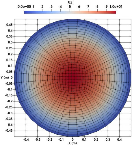
The considered verification case is sketched in Figure 1. The entrance and exit planes of the pipe refer to z = 0 and $z_{max}=2$ m. The pipe radius reads R = 0.5 m. The fully developed axial velocity profile of the laminar flow utilizes $U_{max}=10$ m/s. The fluid properties are selected based on a prescribed Reynolds number of $\mathrm{R}\mathrm{e}=2UR/\nu =2000$, where U and ν refer to the bulk velocity and kinematic viscosity, respectively. The three-dimensional geometry is discretized with approximately 75 k control volumes on a structured grid. A cross-section of the computational grid employed is shown in Figure 2.

Figure 1. Sketch of the pipe flow benchmark.

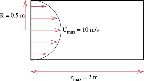
Figure 2. Cross-section of the pipe mesh coloured with the axial velocity.

Due to the decoupled nature of the adjoint hemolysis Equation (26(26) $\begin{array}{rl}{\hat{R}}^H& =u_j\frac{\mathrm{\partial }\hat{h}}{\mathrm{\partial }{x}_j}-C^{\frac{1}{\text{β}}}{\overline{\tau }}^{\frac{\alpha }{\text{β}}}\hat{h}=0.\end{array}$(26) ), an analytical solution can be stated using the analytical primal flow solution (35(35) $\begin{array}{rl}& u_z\left(r\right)=U_{max}\left(1-{\left(\frac{r}{R}\right)}^2\right),H(r,z)=C\frac{{\overline{\tau }}^{\alpha }{z}^{\text{β}}}{u_z^{\text{β}}},\\ & \overline{\tau }\left(r\right)=2\mu U_{max}\frac{r}{R^2},\end{array}$(35) ), viz. (36) $u_z\frac{\mathrm{d}\hat{h}}{\mathrm{d}z}-C^{\frac{1}{\text{β}}}{\overline{\tau }}^{\frac{\alpha }{\text{β}}}\hat{h}=0.$(36) If we abbreviate $\mathrm{\Lambda }=C^{\frac{1}{\text{β}}}{\overline{\tau }}^{\frac{\alpha }{\text{β}}}$, then the solution of (36(36) $u_z\frac{\mathrm{d}\hat{h}}{\mathrm{d}z}-C^{\frac{1}{\text{β}}}{\overline{\tau }}^{\frac{\alpha }{\text{β}}}\hat{h}=0.$(36) ) reads (37) $\hat{h}=K{\mathrm{e}}^{\frac{\mathrm{\Lambda }}{u_z}z},$(37) The integration constant K is calculated based on the BCs of the adjoint hemolysis equation which results from satisfying the final expression in (27(27) $\begin{array}{rl}{\hat{u}}_i{n}_i& =0\mathrm{a}\mathrm{l}\mathrm{o}\mathrm{n}\mathrm{g}\mathrm{\Gamma },\\ & -\hat{p}{n}_i+\rho {\hat{u}}_i{u}_j{n}_j+\mu \frac{\mathrm{\partial }{\hat{u}}_i}{\mathrm{\partial }{x}_j}{n}_j+H_L\hat{h}{n}_i-\hat{h}{B}_{ij}{n}_j=0\\ & \mathrm{a}\mathrm{l}\mathrm{o}\mathrm{n}\mathrm{g}\mathrm{\Gamma }\setminus {\mathrm{\Gamma }}_{\mathrm{o}\mathrm{u}\mathrm{t}},\\ & -\hat{p}{n}_i+\rho {\hat{u}}_i{u}_j{n}_j+\mu \frac{\mathrm{\partial }{\hat{u}}_i}{\mathrm{\partial }{x}_j}{n}_j+H_L\hat{h}{n}_i-\hat{h}{B}_{ij}{n}_j\\ & +\rho H_L^{\text{β}}{n}_i=0\mathrm{a}\mathrm{l}\mathrm{o}\mathrm{n}\mathrm{g}{\mathrm{\Gamma }}_{\mathrm{o}\mathrm{u}\mathrm{t}},\\ & -\hat{h}\left(u_j{n}_j\right)=0\mathrm{a}\mathrm{l}\mathrm{o}\mathrm{n}\mathrm{g}\mathrm{\Gamma }\setminus {\mathrm{\Gamma }}_{\mathrm{o}\mathrm{u}\mathrm{t}},\\ & \hat{h}+\rho \text{β}{H}_L^{(\text{β}-1)}=0\mathrm{a}\mathrm{l}\mathrm{o}\mathrm{n}\mathrm{g}{\mathrm{\Gamma }}_{\mathrm{o}\mathrm{u}\mathrm{t}}.\end{array}$(27) ) and demands $\hat{h}{|}_{\mathrm{o}\mathrm{u}\mathrm{t}}=-\rho \text{β}{H}_L^{\text{β}-1}{|}_{\mathrm{o}\mathrm{u}\mathrm{t}}$. Finally, the adjoint hemolysis field in a fully developed pipe flow reads (38) $\hat{h}=-\rho \text{β}{H}_L^{\text{β}-1}{|}_{\mathrm{o}\mathrm{u}\mathrm{t}}{\mathrm{e}}^{\frac{\mathrm{\Lambda }}{u_z}(z-z_{max})},$(38) where $H_L{|}_{\mathrm{o}\mathrm{u}\mathrm{t}}$ is calculated by setting $z=z_{max}$ in (35(35) $\begin{array}{rl}& u_z\left(r\right)=U_{max}\left(1-{\left(\frac{r}{R}\right)}^2\right),H(r,z)=C\frac{{\overline{\tau }}^{\alpha }{z}^{\text{β}}}{u_z^{\text{β}}},\\ & \overline{\tau }\left(r\right)=2\mu U_{max}\frac{r}{R^2},\end{array}$(35) ) together with $H_L^{\text{β}}=H$.

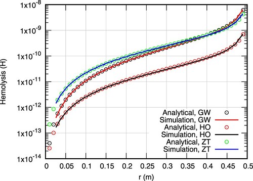
Figure 3 compares the computed primal hemolysis solution against analytical values as calculated by Equation (35(35) $\begin{array}{rl}& u_z\left(r\right)=U_{max}\left(1-{\left(\frac{r}{R}\right)}^2\right),H(r,z)=C\frac{{\overline{\tau }}^{\alpha }{z}^{\text{β}}}{u_z^{\text{β}}},\\ & \overline{\tau }\left(r\right)=2\mu U_{max}\frac{r}{R^2},\end{array}$(35) ). The comparison is realized for all three sets of hemolysis model parameters outlined in Table 1. As can be seen, all computed values are fitting the analytical solutions to a satisfying degree.

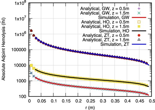
Figure 4 compares the computed adjoint hemolysis field against the analytical solutions (38(38) $\hat{h}=-\rho \text{β}{H}_L^{\text{β}-1}{|}_{\mathrm{o}\mathrm{u}\mathrm{t}}{\mathrm{e}}^{\frac{\mathrm{\Lambda }}{u_z}(z-z_{max})},$(38) ). Due to the nature of the BCs of the adjoint hemolysis equation, the field values are negative and thus the absolute values are presented to support a log-scale of the ordinate. Predictions are nearly identical to analytical solutions for all three set of parameters. Both the primal and adjoint hemolysis solvers are thus considered verified.

Figure 3. Primal hemolysis profiles at z = 1.0 m for three different parameter sets (C, α, β). The notation follows from Table 1. Continuous lines correspond to computations performed for k = 1 while symbols to analytical values.

We would like to remark on the nature of the adjoint hemolysis equation. As can be seen in Figure 4, the adjoint hemolysis profile changes only slightly for different axial positions. The BC at the outlet, which reads $\hat{h}{|}_{\mathrm{o}\mathrm{u}\mathrm{t}}=-\rho \text{β}{H}_L^{\text{β}-1}{|}_{\mathrm{o}\mathrm{u}\mathrm{t}}$, dominates the complete field since all three cases correspond to $\text{β}<1$ and $H_L\ll 1$. To avoid numerical errors that would arise for $H_L{|}_{\mathrm{o}\mathrm{u}\mathrm{t}}=0$, the BCs on the outlet is reformulated to $\hat{h}{|}_{\mathrm{o}\mathrm{u}\mathrm{t}}=-\rho \text{β}(H_L+ϵ{)}^{(\text{β}-1)}{|}_{\mathrm{o}\mathrm{u}\mathrm{t}}$, where $ϵ={10}^{-20}$. Based on the previous comments, one could assume that applying the bulk outlet adjoint hemolysis profile to the whole field suffices. However, due to the existence of the final two terms in the adjoint momentum, (cf. Equation (25(25) $\begin{array}{rl}{\hat{R}}_i^u& =\rho {\hat{u}}_j\frac{\mathrm{\partial }{u}_j}{\mathrm{\partial }{x}_i}-\rho u_j\frac{\mathrm{\partial }{\hat{u}}_i}{\mathrm{\partial }{x}_j}-\frac{\mathrm{\partial }}{\mathrm{\partial }{x}_j}\left(2\mu {\hat{S}}_{ij}-\hat{p}{\delta }_{ij}\right)\\ & +\frac{\mathrm{\partial }\left(\hat{h}{B}_{ij}\right)}{\mathrm{\partial }{x}_j}-H_L\frac{\mathrm{\partial }\hat{h}}{\mathrm{\partial }{x}_i}=0,\end{array}$(25) )), this assumption would fall short on capturing the conceptual description of the complete model.

Figure 4. Magnitude of adjoint hemolysis profiles for three different parameter sets (C, α, β). Notation as in Figure 3. Analytical results are reported for two longitudinal positions, z = 0.5 and z = 1.5 m.

3.2. Sensitivity validation

The goal of the primal-adjoint simulation is the computation of the surface sensitivity (shape derivative) through Equation (32(32) $S_L={\int }_{{\mathrm{\Gamma }}_D}-\left[\mu \frac{\mathrm{\partial }{u}_{i\left(t\right)}}{\mathrm{\partial }n}\frac{\mathrm{\partial }{\hat{u}}_{i\left(t\right)}}{\mathrm{\partial }n}\right]\mathrm{d}\mathrm{\Gamma },$(32) ). It is thus important to investigate the accuracy of the computed sensitivity. In order to realize this, the computed shape derivative is compared against locally evaluated second order accurate finite differences (Kröger & Rung, 2015; Papadimitriou & Giannakoglou, 2007), viz. (39) ${\delta }_{c_i}J=\frac{\left[J(c_i+ϵn_i)-J(c_i-ϵn_i)\right]}{2ϵ}.$(39) Here $c_i$ represents discrete points of the control, ϵ is the magnitude of the perturbation and $n_i$ is the normal vector at $c_i$. In practise, the study is realized by deforming the boundary faces of the discretized geometry into their normal direction with a magnitude equal to ϵ. The local boundary perturbations are then transported into the domain based on (34(34) $\begin{array}{rl}& \frac{\mathrm{\partial }}{\mathrm{\partial }{x}_j}\left[q\frac{\mathrm{\partial }{d}_i}{\mathrm{\partial }{x}_j}\right]=0\mathrm{i}\mathrm{n}\mathrm{\Omega },d_i=-G_{L_i}\mathrm{a}\mathrm{l}\mathrm{o}\mathrm{n}\mathrm{g}{\mathrm{\Gamma }}_D,\\ & d_i=0\mathrm{a}\mathrm{l}\mathrm{o}\mathrm{n}\mathrm{g}\mathrm{\Gamma }\setminus {\mathrm{\Gamma }}_D.\end{array}$(34) ). Figure 5 presents a schematic of the considered symmetric geometry. In specific, the design section (${\mathrm{\Gamma }}_D$) follows from $y=A(\sin (\frac{\pi }{L}x-\frac{\pi }{1000}){)}^4$, where A is the height of the bump, L is the length of the design surface and $L/A=20$. The domain is discretized with approximately 70 k control volumes on a structured grid which is refined in normal as well as tangential direction towards the wall and ${\mathrm{\Gamma }}_D$. A detail of the utilized grid along a part of the design section is shown in Figure 6.

Figure 5. Geometry for the 2D FD study. Dashed lines correspond to the design walls (${\mathrm{\Gamma }}_D$) while continuous lines indicate bounded walls (${\mathrm{\Gamma }}_B$). All dimensions in (m). (Figure not in scale).

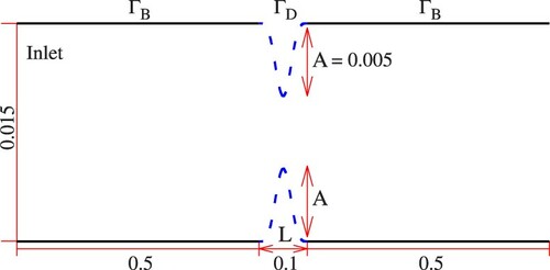
Figure 6. Detail of the utilized grid for the FD study at the section $x\in [0.55-0.575]$ m, where x = 0 refers to the inlet and x = 1.1 to the outlet. (Figure in scale).

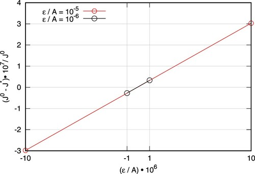
The study is conducted for a parabolic inlet velocity profile with $U_{max}=0.3$ m/s. The fluid properties ($\rho ,\mu$) are assigned to unity to simplify the study. The results of the FD study are shown in Figure 7 for two perturbation magnitudes, ϵ, at 20 selected discrete positions. The overall agreement between the computed adjoint shape derivative and the FD results is very good. Furthermore, as shown in Figure 8 the computed objective functional, on the perturbed shapes, exhibits a linear behaviour w.r.t the perturbation size.

Figure 7. Comparison of sensitivity predicted by Equation (32(32) $S_L={\int }_{{\mathrm{\Gamma }}_D}-\left[\mu \frac{\mathrm{\partial }{u}_{i\left(t\right)}}{\mathrm{\partial }n}\frac{\mathrm{\partial }{\hat{u}}_{i\left(t\right)}}{\mathrm{\partial }n}\right]\mathrm{d}\mathrm{\Gamma },$(32) ) (continuous line) and computed from FD, Equation (39(39) ${\delta }_{c_i}J=\frac{\left[J(c_i+ϵn_i)-J(c_i-ϵn_i)\right]}{2ϵ}.$(39) ), for $ϵ/A={10}^{-6}$ (circles) and $ϵ/A={10}^{-5}$ (triangles).

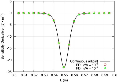
Figure 8. Influence of perturbation size ϵ on FD results at $x=0.55$ m. $J^0$ and $J^{\ast }$ represent the objective functional of the unperturbed and perturbed shapes, respectively.

Overall, the study validates, on a preliminary basis, the accuracy of the adjoint method, as presented within this work.

4. Application

Having assessed the code implementation and the reliability of the computed sensitivity, the approach is put to the test by considering a complete optimization process on a 3D geometry. The latter corresponds to a benchmark model, designed by a technical committee to include flow phenomena related to blood damage in medical devices (Stewart et al., 2012).

4.1. Investigated configuration

The geometry under consideration shares characteristics of many blood-carrying medical devices. It includes sections where the flow is accelerating or decelerating, where re-circulation and significant variations in shear stress occur. All of these phenomena are believed to be related to blood damage in medical devices (Stewart et al., 2012). A merit of the adjoint method is that it stems from the primal (physical) problem. It is therefore capable of shedding light into areas of potentially elevated blood-damage capacity. Areas on which an accumulated shape sensitivity – which is ultimately linked to the displacement field – is identified are expected to be physically relevant to the problem of hemolysis in general. This is shown in Figure 13, where the increase of the maximum hemolysis (which is an output of the primal solver) along the design surface is accompanied by an increase on the displacement field (which is ultimately an output of both the primal and adjoint solution). Therefore, even though there is no direct contribution from the primal hemolysis to the shape sensitivity, the necessary information are preserved. The different shape of the two plots is attributed to the opposite convective nature of the primal and adjoint problems. On the one hand, hemolysis, being convected by the primal velocity, develops in a concave manner due to the physical nature of the flow. On the other hand, the displacement field is a consequence of the sensitivity derivative, cf. Equation (32(32) $S_L={\int }_{{\mathrm{\Gamma }}_D}-\left[\mu \frac{\mathrm{\partial }{u}_{i\left(t\right)}}{\mathrm{\partial }n}\frac{\mathrm{\partial }{\hat{u}}_{i\left(t\right)}}{\mathrm{\partial }n}\right]\mathrm{d}\mathrm{\Gamma },$(32) ), which accounts for the near wall gradient of both primal and adjoint velocity. Due to the reversed flow of the adjoint system the sudden expansion acts as a sudden contraction and the adjoint components of Equation (32(32) $S_L={\int }_{{\mathrm{\Gamma }}_D}-\left[\mu \frac{\mathrm{\partial }{u}_{i\left(t\right)}}{\mathrm{\partial }n}\frac{\mathrm{\partial }{\hat{u}}_{i\left(t\right)}}{\mathrm{\partial }n}\right]\mathrm{d}\mathrm{\Gamma },$(32) ) mirror the primal ones. The inner product of primal and adjoint velocity gradients results in the convex behavior of displacement shown in Figure 13.

Geometrical details of the model are presented in Figure 9. The wall boundary is again split into two parts, ${\mathrm{\Gamma }}_D$ and ${\mathrm{\Gamma }}_B$, as was done in the previous section. The inlet and outlet tubes are considered to be bounded, since their shape is believed to be trivial to the blood damage capacity. The remaining structure is classified as ${\mathrm{\Gamma }}_D$ and presented in blue.

Figure 9. Top: Sketch of the investigated geometry, adapted from Stewart et al. (2012). Presented with dashed lines are the sections free for design. The remaining structure is bounded to its initial configuration. Bottom: Detail of the computational grid on a longitudinal section of the geometry near the design surface.

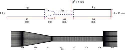
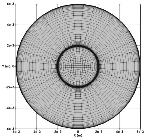
The geometry is discretized with approximately 1 million control volumes on a butterfly-like structured grid. The mesh is gradually condensed near the walls, cf. Figures 10 and 11, to adequately resolve relevant flow phenomena and also near the ${\mathrm{\Gamma }}_D$ section (Figure 9), to ensure an accurate computation of the sensitivity. As can be seen in Figure 11, the grid is additionally refined in the throat region to sufficiently capture the free shear flow, occurring by the jet exiting the throat.

Figure 10. Cross-sectional view of the grid near the inlet.

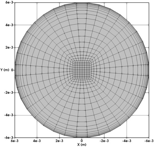
Figure 11. Cross-sectional view of the grid near the outlet.

The fluid's density and dynamic viscosity are set to 1056 kg/m${}^3$ and $3.5\cdot {10}^{-3}$ Pa.s, respectively, representing blood under physiological conditions. A fully developed laminar axial velocity profile is prescribed at the inlet of the geometry, based on (35(35) $\begin{array}{rl}& u_z\left(r\right)=U_{max}\left(1-{\left(\frac{r}{R}\right)}^2\right),H(r,z)=C\frac{{\overline{\tau }}^{\alpha }{z}^{\text{β}}}{u_z^{\text{β}}},\\ & \overline{\tau }\left(r\right)=2\mu U_{max}\frac{r}{R^2},\end{array}$(35) ), so that the Reynolds number at the throat reads $R{e}_T=500$. As regards the hemolysis-prediction model, the utilized set of parameters corresponds to GW (cf. Table 1) and we employ k = 1 for the computation of the scalar stress representation (4(4) $\overline{\tau }=\sqrt{-k{I}_{{\tau }_2}}\mathrm{w}\mathrm{i}\mathrm{t}\mathrm{h}{I}_{{\tau }_2}=\frac{1}{2}\left[\left(tr({\tau }_{ij}{)}^2-tr({\tau }_{ij}^2)\right)\right].$(4) ). The diffusion terms in the adjoint and primal momentum equations are discretized using the second-order accurate central difference scheme. The convective term in the primal momentum is discretized through the higher order Quadratic Upstream Interpolation of Convective Kinematics (QUICK) scheme. Due to the negative sign of the convection term in the adjoint momentum (cf. Equation (25(25) $\begin{array}{rl}{\hat{R}}_i^u& =\rho {\hat{u}}_j\frac{\mathrm{\partial }{u}_j}{\mathrm{\partial }{x}_i}-\rho u_j\frac{\mathrm{\partial }{\hat{u}}_i}{\mathrm{\partial }{x}_j}-\frac{\mathrm{\partial }}{\mathrm{\partial }{x}_j}\left(2\mu {\hat{S}}_{ij}-\hat{p}{\delta }_{ij}\right)\\ & +\frac{\mathrm{\partial }\left(\hat{h}{B}_{ij}\right)}{\mathrm{\partial }{x}_j}-H_L\frac{\mathrm{\partial }\hat{h}}{\mathrm{\partial }{x}_i}=0,\end{array}$(25) )) the direction of the convective transport is opposite to the original PDE. The corresponding downwind analogy to QUICK is, thus, used for the convection term in the adjoint momentum (Stück &Rung, 2013).

4.2. Shape optimization study

The optimization study resulted in 50 design candidates. The employed smoothing parameter value (33(33) $G_{L_i}-{\lambda }^2{\mathrm{\Delta }}_{\mathrm{\Gamma }}{G}_{L_i}=S_L{n}_i,$(33) ) reads $\lambda =R^T\sqrt{{10}^3}$, where $R^T$ is the throat radius. To avoid large deformations of the geometry and the grid, the local displacement index field $d_i$ computed from Equation (34(34) $\begin{array}{rl}& \frac{\mathrm{\partial }}{\mathrm{\partial }{x}_j}\left[q\frac{\mathrm{\partial }{d}_i}{\mathrm{\partial }{x}_j}\right]=0\mathrm{i}\mathrm{n}\mathrm{\Omega },d_i=-G_{L_i}\mathrm{a}\mathrm{l}\mathrm{o}\mathrm{n}\mathrm{g}{\mathrm{\Gamma }}_D,\\ & d_i=0\mathrm{a}\mathrm{l}\mathrm{o}\mathrm{n}\mathrm{g}\mathrm{\Gamma }\setminus {\mathrm{\Gamma }}_D.\end{array}$(34) ) was scaled to a user-defined constant maximum value ${\tilde{d}}_{max}$, viz. (40) $\widetilde{d_i}=\frac{d_i}{max\left(d_i\right)}{\tilde{d}}_{max}.$(40) For the study at hand ${\tilde{d}}_{max}/d^T=0.25\cdot {10}^{-2}$.

Figure 12 shows the displacement magnitude on the design surfaces of the structure at hand, after the solution of the first primal and adjoint problem. As can be seen, the displacement is accumulated, almost entirely, at the sudden expansion of the geometry, where the highest values of hemolysis occur (cf. Figure 13). Furthermore, re-circulation is occurring with relatively significant values of upstream mass fluxes after the expansion. This is believed to be one of the causes of hemolysis.

Figure 12. Displacement magnitude field as computed by Equation (40(40) $\widetilde{d_i}=\frac{d_i}{max\left(d_i\right)}{\tilde{d}}_{max}.$(40) ) after the first primal and adjoint simulations. The field is scaled by the maximum value. Areas shown in red correspond to high displacement values (for reference to colours, the reader is prompted to the online version of the article).

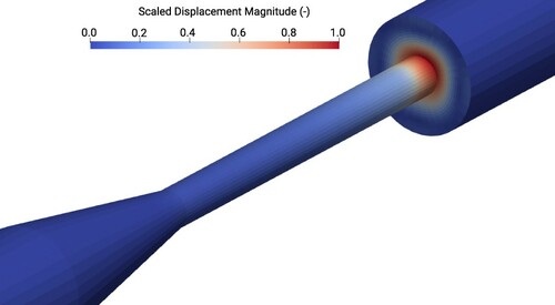
Figure 13. Maximum values of ϕ along radial cuts on ${\mathrm{\Gamma }}_D$ after the first primal and adjoint simulations, where ϕ corresponds to the displacement magnitude and hemolysis for the continuous and dashed lines, respectively. Values are scaled between [0-1] for visualization purposes.

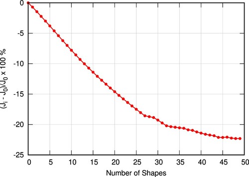
The optimization history is shown in Figure 15. It can be seen that the optimization starts converging after approximately 40 shapes. The final shape results in a relative reduction of the objective functional by 22%. A comparison of the initial and the optimized shape is displayed in Figure 14. The optimization algorithm, proceeded into widening and relatively smoothing the sudden expansion of the geometry. In specific, in the optimized shape, the diameter at the end of the throat (sudden expansion) increases by 20%, compared to the initial value.

Figure 16 shows the predicted and measured axial velocity along the centerline of the initial geometry. Similarly, Figures 17 and 18 depict the axial velocity profiles of two cross-sections in the vicinity of the sudden expansion. Experimental data were extracted from the average over a few sample experiments of Stewart et al. (2012), as reported in https://fdacfd.nci.nih.gov. An obvious deviation between the measured and the predicted volume flux is seen in Figures 17 and 18. Therefore, supplementary computations were performed for the initial geometry which match the average estimated experimental volume flux. The related (volume-flux scaled) computational results are indicated by the dashed lines in Figures 16–18. They reveal a fair predictive agreement and support the validity of the subsequent optimization study.

Figure 14. Projection of ${\mathrm{\Gamma }}_D$ on a 2D plane. Dashed line illustrates the outline of the final optimized shape ($c^{50}$) while continuous line corresponds to the initial shape. The bottom part is symmetric w.r.t the symmetry line. Axes not in scale.

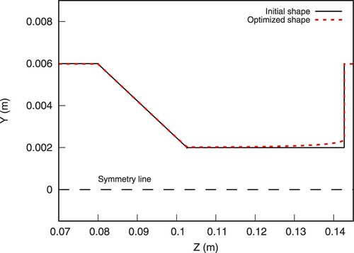
Figure 15. Optimization convergence. $J_i$ denotes the objective functional as computed for each shape $c^i$ and $J_0$ denotes the same value for the initial shape, $c^0$. Points illustrate the computed quantity at each discrete shape.

The optimized shape results in a smaller maximum value of the axial velocity as can be seen in Figure 16. At the same time, nonetheless, the flow inside the bounded portions of the structure ($z\in [0:0.12]$ m) remains relatively unchanged as shown on the same figure. This is important in terms of biomedical applications due to their ultimate goal of realizing a sensitive task. However, due to the smoothing of the expansion zone, the velocity profiles are changed in the perturbed section of the geometry (cf. Figures 17 and 18). The velocity profile of the optimized shape is smoothed near the wall region resulting in substantially lower shear stresses.

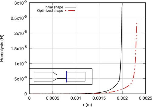
Subsequently, due to the direct relation between shear stresses and hemolysis induction, the maximum values of hemolysis in the flow is reduced in the perturbed section of the structure, which is also the area on which the maximum values are identified in the initial shape. A direct comparison of the hemolysis profiles at two cross sections of the initial and final geometry is presented in Figures 19 and 20.

Figure 16. Comparison of axial centerline velocities (r = 0) obtained from computations of the initial (continuous line) and the optimized (dashed-continuous line) shape Re = 500, supplemented by averaged experimental data reported by Stewart et al. (2012). For the initial shape, a second computed result is displayed (dashed line) which corresponds to an adjusted volume flux as suggested by averaged experimental data. Coordinate Z = 0 corresponds to the model's inlet.

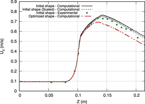
Figure 17. Comparison of axial velocity profiles at Z = 0.135 m obtained from computations of the initial (continuous line) and the optimized (dashed-continuous line) shape for Re = 500, supplemented by averaged experimental data for the initial geometry reported by Stewart et al. (2012) (symbols). Dashed line as in Figure 16.

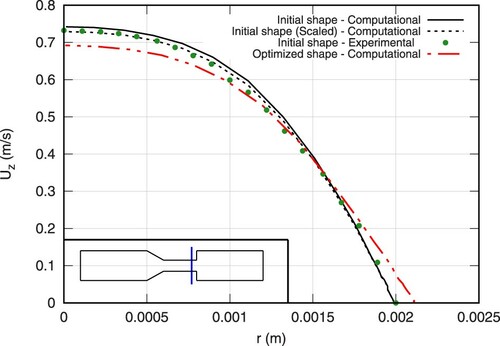
Figure 18. Comparison of axial velocity profiles at Z = 0.142 m obtained from computations of the initial (continuous line) and the optimized (continuous-dashed line) shape for Re = 500, supplemented by averaged experimental data for the initial geometry reported by Stewart et al. (2012) (symbols). Dashed line as in Figure 16.

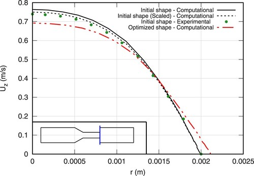
Figure 19. Hemolysis cross-sectional profiles for initial (continuous line) and optimized (continuous-dashed line) shape at Z = 0.135 m.

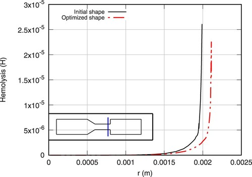
Figure 20. Hemolysis cross-sectional profiles for initial (continuous line) and optimized (continuous-dashed line) shape at Z = 0.142 m, corresponding to the final nodes before the sudden expansion of the initial shape.

As described in the previous section, the optimization utilized a specific set of parameters for the primal hemolysis model. It is interesting, therefore, to examine the performance of the optimized shape for other sets of hemolysis specific parameters. As shown in Figure 21 (Table 3), for any choice of parameters mentioned in Table 1, the optimal shape always outperforms the initial one in terms of flow-induced hemolysis. In specific, the most significant improvement occurs for the employed set of parameters during the optimization run, namely GW, while the value of k is relatively trivial w.r.t the improvement. This shows a robustness of the method in terms of user-defined values.

Figure 21. Computed values of $H_{\mathrm{i}\mathrm{n}\mathrm{d}\mathrm{e}\mathrm{x}}$ (Equation (9(9) $H_{index}=\frac{{\int }_{{\mathrm{\Gamma }}_{\mathrm{o}\mathrm{u}\mathrm{t}}}H\rho u_j{n}_j\mathrm{d}\mathrm{\Gamma }}{{\int }_{{\mathrm{\Gamma }}_{\mathrm{o}\mathrm{u}\mathrm{t}}}\rho u_j{n}_j\mathrm{d}\mathrm{\Gamma }}=\frac{{\int }_{{\mathrm{\Gamma }}_{\mathrm{o}\mathrm{u}\mathrm{t}}}{H}_L^{\text{β}}\rho u_j{n}_j\mathrm{d}\mathrm{\Gamma }}{{\int }_{{\mathrm{\Gamma }}_{\mathrm{o}\mathrm{u}\mathrm{t}}}\rho u_j{n}_j\mathrm{d}\mathrm{\Gamma }}.$(9) )) for different set of parameters (cf. Table 1) and different k values (Equation (cf. (4(4) $\overline{\tau }=\sqrt{-k{I}_{{\tau }_2}}\mathrm{w}\mathrm{i}\mathrm{t}\mathrm{h}{I}_{{\tau }_2}=\frac{1}{2}\left[\left(tr({\tau }_{ij}{)}^2-tr({\tau }_{ij}^2)\right)\right].$(4) ))). For each set of parameters and k value the percentage decrease of the objective on the initial w.r.t to the optimized shape is shown next to points. Y-axis in logscale.

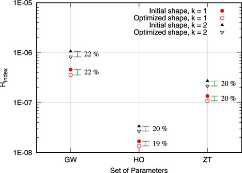
Table 3. Exact values of Figure 21.

Shape	Param.	k	$H_{\mathrm{i}\mathrm{n}\mathrm{d}\mathrm{e}\mathrm{x}}$
Initial	GW	1	0.460E−6
Optimized	GW	1	0.359E−6
Initial	GW	2	0.106E−5
Optimized	GW	2	0.826E−6
Initial	HO	1	0.169E−7
Optimized	HO	1	0.136E−7
Initial	HO	2	0.337E−7
Optimized	HO	2	0.270E−7
Initial	ZT	1	0.135E−6
Optimized	ZT	1	0.109E−6
Initial	ZT	2	0.271E−6
Optimized	ZT	2	0.215E−6

5. Conclusions and outlook

This paper discusses a continuous adjoint approach for shape optimization targeting to minimize flow-induced hemolysis in biomedical applications. A detailed derivation of the adjoint model which stems from the original power-law formulation for hemolysis prediction is reported.

A benchmark problem is examined to verify the numerical implementation of the primal and adjoint hemolysis equations. The numerical results compare favorably against those deduced from analytical solutions of the problem. The validity of the derived sensitivity is put to the test on a two-dimensional stenosed geometry on which a FD study is realized. The continuous computed sensitivity from the adjoint method is compared against the locally evaluated results of the FD study and a fitness is found.

The complete optimization method based on the derived adjoint equations is applied on a three-dimensional geometry, specifically designed to include flow peculiarities, related to blood damage in medical devices. An optimized shape, in 50 shape updates, able to reduce the numerically predicted flow-induced hemolysis by 22% is found. The performance of the optimized shape, in terms of blood damage, is then tested for different hemolysis-related parameters. It is found that in all cases, the optimized geometry outperforms the initial one.

Based on the above we would like to highlight the following conclusions from this study:

1. A frequently employed parameterized, stress-related hemolysis assessment model can be casted into a PDE framework that represents a weak (one-way) coupling to the fluid dynamic PDEs and serves as a starting point for a continuous adjoint formulation of the coupled problem.

2. The choice of parameters ($C,\alpha ,\text{β}$ and k) employed by the computational hemolysis model should be based on the physics of the investigated case or validation data obtained from experiments.

3. Similar to the primal flow, the dual flow is also one-way coupled, however in a reversed sense. This makes its computational implementation a relatively simple task, provided that an adjoint solver already exists.

4. The primal coupling relations translate into a corresponding dual coupling, where the value of primal hemolysis indicator function at the inlet and outlet planes drives the dual flow, in an analogy to pressure-driven duct flows.

5. The proposed optimization method was found to be fairly robust to the choice of parameters employed by the hemolysis model. Due to the uncertainty inherent to such parameter values, the robustness of the optimizer is considered significant by the authors.

Overall, the reported method poses great potential for minimizing flow-induced hemolysis, in silico conditions, due to its computational efficiency. At the same time, however, blood flows can exhibit further peculiarities such as elasticity of the surrounding structure, non-Newtonian properties or occurrence of turbulence. The aforementioned phenomena are not considered in this work. Nevertheless, the adjoint shape optimization method suggested in this paper constitutes a sound basis for further studies into hemolysis minimizing geometries. Future work will target the extension of the method to Fluid Structure Interaction (FSI). The ambiguous impact of turbulence on the hemolysis induction phenomenon should also be investigated by the adjoint approach. Finally, an extension of the adjoint model to include non-Newtonian properties of the fluid, which are more adequate to correctly capture the blood flow with low shear rates, is intended.

Acknowledgments

The current work is part of the research training group ‘Simulation-Based Design Optimization of Dynamic Systems Under Uncertainties’ (SENSUS) funded by the state of Hamburg under the aegis of the Landesforschungsförderungs-Project LFF-GK11. Selected computations were performed with resources provided by the North-German Supercomputing Alliance (HLRN). This support is gratefully acknowledged by the authors. Finally, the publishing fees were covered by the funding programme ‘Open Access Publishing’ of Hamburg University of Technology (TUHH), which we gratefully acknowledge.

Disclosure statement

No potential conflict of interest was reported by the authors.

Additional information

Funding

The current work is part of the research training group ‘Simulation-Based Design Optimization of Dynamic Systems Under Uncertainties’ (SENSUS) funded by the State of Hamburg [Landesforschungsförderungs-Project LFF- GK11]. Publishing fees were covered by the Funding Programme ‘Open Access Publishing’ of Hamburg University of Technology (TUHH).

Appendix.

Assisting information for the adjoint system

Staying true to the notation of Section 2.2.1, the derivation of the directional derivatives of $I_k$, with k = 1,.., 4, is briefly presented herein. The process to arrive at the adjoint Equations (24(24) $\begin{array}{rl}{\hat{R}}^p& =-\frac{\mathrm{\partial }{\hat{u}}_i}{\mathrm{\partial }{x}_i}=0,\end{array}$(24) )–(26(26) $\begin{array}{rl}{\hat{R}}^H& =u_j\frac{\mathrm{\partial }\hat{h}}{\mathrm{\partial }{x}_j}-C^{\frac{1}{\text{β}}}{\overline{\tau }}^{\frac{\alpha }{\text{β}}}\hat{h}=0.\end{array}$(26) ) is also illustrated.

For $I_1$ : $I_1(\hat{p},u_i,\mathrm{\Omega })={\int }_{\mathrm{\Omega }}\hat{p}\left(-\frac{\mathrm{\partial }{u}_j}{\mathrm{\partial }{x}_j}\right)\mathrm{d}\mathrm{\Omega }.$Since $I_1$ does not directly depend on p and $H_L$ it follows (A1) ${\delta }_p{I}_1\cdot \delta p={\delta }_{H_L}{I}_1\cdot \delta H_L=0,$(A1) while for the variation in the direction of $u_i$ (A2) ${\delta }_{u_i}{I}_1\cdot \delta u_i=-{\int }_{\mathrm{\Gamma }}\left(\delta u_i{n}_i\right)\hat{p}\mathrm{d}\mathrm{\Gamma }+{\int }_{\mathrm{\Omega }}\left(\delta u_i\right)\frac{\mathrm{\partial }\hat{p}}{\mathrm{\partial }{x}_i}\mathrm{d}\mathrm{\Omega }.$(A2) For $I_2$ : $I_2({\hat{u}}_i,u_i,\mathrm{\Omega })={\int }_{\mathrm{\Omega }}{\hat{u}}_i\left(\rho u_j\frac{\mathrm{\partial }{u}_i}{\mathrm{\partial }{x}_j}\right)\mathrm{d}\mathrm{\Omega }.$Similarly to $I_1$ (A3) ${\delta }_p{I}_2\cdot \delta p={\delta }_{H_L}{I}_2\cdot \delta H_L=0$(A3) and for its variation on the direction of $u_i$ (A4) $\begin{array}{rl}{\delta }_{u_i}{I}_2\cdot \delta u_i& ={\int }_{\mathrm{\Gamma }}\delta u_i{\hat{u}}_i\rho \left(u_j{n}_j\right)\mathrm{d}\mathrm{\Gamma }\\ & -{\int }_{\mathrm{\Omega }}\left(\delta u_i\right)\left(u_j\rho \frac{\mathrm{\partial }{\hat{u}}_i}{\mathrm{\partial }{x}_j}-{\hat{u}}_j\rho \frac{\mathrm{\partial }{u}_j}{\mathrm{\partial }{x}_i}\right)\mathrm{d}\mathrm{\Omega }.\end{array}$(A4) For $I_3$ : $I_3({\hat{u}}_i,u_i,\mathrm{\Omega })={\int }_{\mathrm{\Omega }}{\hat{u}}_i\left(-\frac{\mathrm{\partial }}{\mathrm{\partial }{x}_j}\left(2\mu S_{ij}\right)\right)\mathrm{d}\mathrm{\Omega }.$As before (A5) $\begin{array}{rl}{\delta }_p{I}_3\cdot \delta p& ={\delta }_{H_L}{I}_3\cdot \delta H_L=0,\end{array}$(A5) (A6) $\begin{array}{rl}{\delta }_{u_i}{I}_3\cdot \delta u_i& =\underset{{\mathrm{\Gamma }}_1}{\underbrace{-{\int }_{\mathrm{\Gamma }}{\hat{u}}_i\mu \left(\frac{\mathrm{\partial }\delta u_i}{\mathrm{\partial }{x}_j}+\frac{\mathrm{\partial }\delta u_j}{\mathrm{\partial }{x}_i}\right)n_j\mathrm{d}\mathrm{\Gamma }}}\\ & +\underset{I_3^{\ast }}{\underbrace{{\int }_{\mathrm{\Omega }}\frac{\mathrm{\partial }{\hat{u}}_i}{\mathrm{\partial }{x}_j}\mu \left(\frac{\mathrm{\partial }\delta u_i}{\mathrm{\partial }{x}_j}+\frac{\mathrm{\partial }\delta u_j}{\mathrm{\partial }{x}_i}\right)\mathrm{d}\mathrm{\Omega }}},\end{array}$(A6) where $I_3^{\ast }$ can be expanded further using a second integration by parts as (A7) $\begin{array}{rl}{I}_3^{\ast }& ={\int }_{\mathrm{\Omega }}\frac{\mathrm{\partial }{\hat{u}}_i}{\mathrm{\partial }{x}_j}\mu \frac{\mathrm{\partial }\delta u_i}{\mathrm{\partial }{x}_j}\mathrm{d}\mathrm{\Omega }+{\int }_{\mathrm{\Omega }}\frac{\mathrm{\partial }{\hat{u}}_i}{\mathrm{\partial }{x}_j}\mu \frac{\mathrm{\partial }\delta u_j}{\mathrm{\partial }{x}_i}\mathrm{d}\mathrm{\Omega }\\ & =\underset{{\mathrm{\Gamma }}_2}{\underbrace{{\int }_{\mathrm{\Gamma }}\left(\delta u_i\right)\mu \left[\frac{\mathrm{\partial }{\hat{u}}_i}{\mathrm{\partial }{x}_j}+\frac{\mathrm{\partial }{\hat{u}}_j}{\mathrm{\partial }{x}_i}\right]n_j\mathrm{d}\mathrm{\Gamma }}}\\ & -{\int }_{\mathrm{\Omega }}\left(\delta u_i\right)\frac{\mathrm{\partial }}{\mathrm{\partial }{x}_j}\left[\mu \left(\frac{\mathrm{\partial }{\hat{u}}_i}{\mathrm{\partial }{x}_j}+\frac{\mathrm{\partial }{\hat{u}}_j}{\mathrm{\partial }{x}_i}\right)\right]\mathrm{d}\mathrm{\Omega }.\end{array}$(A7) Now, ${\mathrm{\Gamma }}_1+{\mathrm{\Gamma }}_2$ are subject to even further expansion (A8) $\begin{array}{rl}{\mathrm{\Gamma }}_1+{\mathrm{\Gamma }}_2& ={\int }_{\mathrm{\Gamma }}\mu n_j\left(\frac{\mathrm{\partial }{\hat{u}}_j}{\mathrm{\partial }{x}_i}\delta u_i-\frac{\mathrm{\partial }\delta u_j}{\mathrm{\partial }{x}_i}{\hat{u}}_i\right)\mathrm{d}\mathrm{\Gamma }\\ & +{\int }_{\mathrm{\Gamma }}\mu n_j\left(\frac{\mathrm{\partial }{\hat{u}}_i}{\mathrm{\partial }{x}_j}\delta u_i-\frac{\mathrm{\partial }\delta u_i}{\mathrm{\partial }{x}_j}{\hat{u}}_i\right)\mathrm{d}\mathrm{\Gamma }.\end{array}$(A8) Expanding the first integral on Equation (A8(A8) $\begin{array}{rl}{\mathrm{\Gamma }}_1+{\mathrm{\Gamma }}_2& ={\int }_{\mathrm{\Gamma }}\mu n_j\left(\frac{\mathrm{\partial }{\hat{u}}_j}{\mathrm{\partial }{x}_i}\delta u_i-\frac{\mathrm{\partial }\delta u_j}{\mathrm{\partial }{x}_i}{\hat{u}}_i\right)\mathrm{d}\mathrm{\Gamma }\\ & +{\int }_{\mathrm{\Gamma }}\mu n_j\left(\frac{\mathrm{\partial }{\hat{u}}_i}{\mathrm{\partial }{x}_j}\delta u_i-\frac{\mathrm{\partial }\delta u_i}{\mathrm{\partial }{x}_j}{\hat{u}}_i\right)\mathrm{d}\mathrm{\Gamma }.\end{array}$(A8) ) leads to (A9) $\begin{array}{rl}& {\int }_{\mathrm{\Gamma }}\mu n_j\left(\frac{\mathrm{\partial }{\hat{u}}_j}{\mathrm{\partial }{x}_i}\delta u_i-\frac{\mathrm{\partial }\delta u_j}{\mathrm{\partial }{x}_i}{\hat{u}}_i\right)\mathrm{d}\mathrm{\Gamma }\\ & ={\int }_{\mathrm{\Gamma }}\mu \frac{\mathrm{\partial }{\hat{u}}_n}{\mathrm{\partial }{x}_i}\delta u_i\mathrm{d}\mathrm{\Gamma }-{\int }_{\mathrm{\Gamma }}\mu \frac{\mathrm{\partial }\delta u_n}{\mathrm{\partial }{x}_i}{\hat{u}}_i\mathrm{d}\mathrm{\Gamma }\\ & ={\left[\mu {\hat{u}}_n\underset{\delta u_n}{\underbrace{\delta u_i{n}_i}}\right]}_{\mathrm{\partial }\mathrm{\Gamma }}-{\left[\mu \underset{{\hat{u}}_n}{\underbrace{{\hat{u}}_i{n}_i}}\delta u_n\right]}_{\mathrm{\partial }\mathrm{\Gamma }}\\ & -{\int }_{\mathrm{\Gamma }}{\hat{u}}_n\mu \frac{\mathrm{\partial }\delta u_i}{\delta x_i}\mathrm{d}\mathrm{\Gamma }+{\int }_{\mathrm{\Gamma }}\delta u_n\mu \frac{\mathrm{\partial }{\hat{u}}_i}{\mathrm{\partial }{x}_i}\mathrm{d}\mathrm{\Gamma }\\ & =0.\end{array}$(A9) The last two integrals of Equation (A9(A9) $\begin{array}{rl}& {\int }_{\mathrm{\Gamma }}\mu n_j\left(\frac{\mathrm{\partial }{\hat{u}}_j}{\mathrm{\partial }{x}_i}\delta u_i-\frac{\mathrm{\partial }\delta u_j}{\mathrm{\partial }{x}_i}{\hat{u}}_i\right)\mathrm{d}\mathrm{\Gamma }\\ & ={\int }_{\mathrm{\Gamma }}\mu \frac{\mathrm{\partial }{\hat{u}}_n}{\mathrm{\partial }{x}_i}\delta u_i\mathrm{d}\mathrm{\Gamma }-{\int }_{\mathrm{\Gamma }}\mu \frac{\mathrm{\partial }\delta u_n}{\mathrm{\partial }{x}_i}{\hat{u}}_i\mathrm{d}\mathrm{\Gamma }\\ & ={\left[\mu {\hat{u}}_n\underset{\delta u_n}{\underbrace{\delta u_i{n}_i}}\right]}_{\mathrm{\partial }\mathrm{\Gamma }}-{\left[\mu \underset{{\hat{u}}_n}{\underbrace{{\hat{u}}_i{n}_i}}\delta u_n\right]}_{\mathrm{\partial }\mathrm{\Gamma }}\\ & -{\int }_{\mathrm{\Gamma }}{\hat{u}}_n\mu \frac{\mathrm{\partial }\delta u_i}{\delta x_i}\mathrm{d}\mathrm{\Gamma }+{\int }_{\mathrm{\Gamma }}\delta u_n\mu \frac{\mathrm{\partial }{\hat{u}}_i}{\mathrm{\partial }{x}_i}\mathrm{d}\mathrm{\Gamma }\\ & =0.\end{array}$(A9) ) vanish because the primal velocity field is asymptotically divergence-free in the boundary so its variation must be divergence-free too and because we showed that the adjoint velocity must also be divergence-free. Finally, simplifying Equation (A8(A8) $\begin{array}{rl}{\mathrm{\Gamma }}_1+{\mathrm{\Gamma }}_2& ={\int }_{\mathrm{\Gamma }}\mu n_j\left(\frac{\mathrm{\partial }{\hat{u}}_j}{\mathrm{\partial }{x}_i}\delta u_i-\frac{\mathrm{\partial }\delta u_j}{\mathrm{\partial }{x}_i}{\hat{u}}_i\right)\mathrm{d}\mathrm{\Gamma }\\ & +{\int }_{\mathrm{\Gamma }}\mu n_j\left(\frac{\mathrm{\partial }{\hat{u}}_i}{\mathrm{\partial }{x}_j}\delta u_i-\frac{\mathrm{\partial }\delta u_i}{\mathrm{\partial }{x}_j}{\hat{u}}_i\right)\mathrm{d}\mathrm{\Gamma }.\end{array}$(A8) ) through Equation (A9(A9) $\begin{array}{rl}& {\int }_{\mathrm{\Gamma }}\mu n_j\left(\frac{\mathrm{\partial }{\hat{u}}_j}{\mathrm{\partial }{x}_i}\delta u_i-\frac{\mathrm{\partial }\delta u_j}{\mathrm{\partial }{x}_i}{\hat{u}}_i\right)\mathrm{d}\mathrm{\Gamma }\\ & ={\int }_{\mathrm{\Gamma }}\mu \frac{\mathrm{\partial }{\hat{u}}_n}{\mathrm{\partial }{x}_i}\delta u_i\mathrm{d}\mathrm{\Gamma }-{\int }_{\mathrm{\Gamma }}\mu \frac{\mathrm{\partial }\delta u_n}{\mathrm{\partial }{x}_i}{\hat{u}}_i\mathrm{d}\mathrm{\Gamma }\\ & ={\left[\mu {\hat{u}}_n\underset{\delta u_n}{\underbrace{\delta u_i{n}_i}}\right]}_{\mathrm{\partial }\mathrm{\Gamma }}-{\left[\mu \underset{{\hat{u}}_n}{\underbrace{{\hat{u}}_i{n}_i}}\delta u_n\right]}_{\mathrm{\partial }\mathrm{\Gamma }}\\ & -{\int }_{\mathrm{\Gamma }}{\hat{u}}_n\mu \frac{\mathrm{\partial }\delta u_i}{\delta x_i}\mathrm{d}\mathrm{\Gamma }+{\int }_{\mathrm{\Gamma }}\delta u_n\mu \frac{\mathrm{\partial }{\hat{u}}_i}{\mathrm{\partial }{x}_i}\mathrm{d}\mathrm{\Gamma }\\ & =0.\end{array}$(A9) ) and inserting the remaining terms in Equation (A6(A6) $\begin{array}{rl}{\delta }_{u_i}{I}_3\cdot \delta u_i& =\underset{{\mathrm{\Gamma }}_1}{\underbrace{-{\int }_{\mathrm{\Gamma }}{\hat{u}}_i\mu \left(\frac{\mathrm{\partial }\delta u_i}{\mathrm{\partial }{x}_j}+\frac{\mathrm{\partial }\delta u_j}{\mathrm{\partial }{x}_i}\right)n_j\mathrm{d}\mathrm{\Gamma }}}\\ & +\underset{I_3^{\ast }}{\underbrace{{\int }_{\mathrm{\Omega }}\frac{\mathrm{\partial }{\hat{u}}_i}{\mathrm{\partial }{x}_j}\mu \left(\frac{\mathrm{\partial }\delta u_i}{\mathrm{\partial }{x}_j}+\frac{\mathrm{\partial }\delta u_j}{\mathrm{\partial }{x}_i}\right)\mathrm{d}\mathrm{\Omega }}},\end{array}$(A6) ) (A10) $\begin{array}{rl}{\delta }_{u_i}{I}_3\cdot \delta u_i& ={\int }_{\mathrm{\Gamma }}\left(\delta u_i\right)\mu n_j\frac{\mathrm{\partial }{\hat{u}}_i}{\mathrm{\partial }{x}_j}\mathrm{d}\mathrm{\Gamma }-{\int }_{\mathrm{\Gamma }}{\hat{u}}_i\mu n_j\frac{\mathrm{\partial }\delta u_i}{\mathrm{\partial }{x}_j}\mathrm{d}\mathrm{\Gamma }\\ & -{\int }_{\mathrm{\Omega }}\left(\delta u_i\right)\frac{\mathrm{\partial }}{\mathrm{\partial }{x}_j}\left(2\mu {\hat{S}}_{ij}\right)\mathrm{d}\mathrm{\Omega }.\end{array}$(A10) For $I_4$: $I_4({\hat{u}}_i,p,\mathrm{\Omega })={\int }_{\mathrm{\Omega }}{\hat{u}}_i\left(\frac{\mathrm{\partial }p}{\mathrm{\partial }{x}_i}\right)\mathrm{d}\mathrm{\Omega }.$It follows that (A11) ${\delta }_{u_i}{I}_4\cdot \delta u_i={\delta }_{H_L}{I}_4\cdot \delta H_L=0,$(A11) while for the variation in the direction of pressure (A12) ${\delta }_p{I}_4\cdot \delta p={\int }_{\mathrm{\Gamma }}\left(\delta p\right){\hat{u}}_i{n}_i\mathrm{d}\mathrm{\Gamma }-{\int }_{\mathrm{\Omega }}\left(\delta p\right)\frac{\mathrm{\partial }{\hat{u}}_i}{\mathrm{\partial }{x}_i}\mathrm{d}\mathrm{\Omega }.$(A12) Having expressed all sub-integrals in the form of surface and volume integrals we can superpose all contributions (considering also those from the main body of the paper) into the directional derivatives of the Lagrange functional so that (A13) $\begin{array}{rl}{\delta }_p\mathcal{L}\cdot \delta p& ={\int }_{\mathrm{\Gamma }}\left(\delta p\right){\hat{u}}_i{n}_i\mathrm{d}\mathrm{\Gamma }-{\int }_{\mathrm{\Omega }}\left(\delta p\right)\frac{\mathrm{\partial }{\hat{u}}_i}{\mathrm{\partial }{x}_i}\mathrm{d}\mathrm{\Omega },\end{array}$(A13) (A14) $\begin{array}{rl}{\delta }_{u_i}L\cdot \delta u_i& ={\int }_{\mathrm{\Gamma }}\left(\delta u_i\right)\left[-\hat{p}{n}_i+\rho {\hat{u}}_i{u}_j{n}_j+\mu \frac{\mathrm{\partial }{\hat{u}}_i}{\mathrm{\partial }{x}_j}{n}_j\right.\\ & +\left.H_L\hat{h}{n}_i-\hat{h}{B}_{ij}{n}_j+\frac{\mathrm{\partial }{j}_{\mathrm{\Gamma }}}{\mathrm{\partial }{u}_i}\right]\mathrm{d}\mathrm{\Gamma }\\ & +{\int }_{\mathrm{\Omega }}\left(\delta u_i\right)\left[{\hat{u}}_j\rho \frac{\mathrm{\partial }{u}_j}{\mathrm{\partial }{x}_i}-u_j\rho \frac{\mathrm{\partial }{\hat{u}}_i}{\mathrm{\partial }{x}_j}\right.\\ & -\left.\frac{\mathrm{\partial }}{\mathrm{\partial }{x}_j}\left(2\mu {\hat{S}}_{ij}-\hat{p}{\delta }_{ij}\right)+\frac{\mathrm{\partial }\left(\hat{h}{B}_{ij}\right)}{\mathrm{\partial }{x}_j}-H_L\frac{\mathrm{\partial }\hat{h}}{\mathrm{\partial }{x}_i}\right]\mathrm{d}\mathrm{\Omega }\\ & -{\int }_{\mathrm{\Gamma }}\mu {\hat{u}}_i\frac{\mathrm{\partial }\delta u_i}{\mathrm{\partial }{x}_j}{n}_j\mathrm{d}\mathrm{\Gamma },\end{array}$(A14) (A15) $\begin{array}{rl}{\delta }_{H_L}L\cdot \delta H_L& ={\int }_{\mathrm{\Gamma }}\left(\delta H_L\right)\left(\hat{h}\left(u_j{n}_j\right)+\frac{\mathrm{\partial }{j}_{\mathrm{\Gamma }}}{\mathrm{\partial }{H}_L}\right)\mathrm{d}\mathrm{\Gamma }\\ & +{\int }_{\mathrm{\Omega }}\left(\delta H_L\right)\left(u_j\frac{\mathrm{\partial }\hat{h}}{\mathrm{\partial }{x}_j}-C^{\frac{1}{\text{β}}}{\overline{\tau }}^{\frac{a}{b}}\hat{h}\right)\mathrm{d}\mathrm{\Omega }.\end{array}$(A15) Finally, by demanding that the integrals of the form of Equation (23(23) ${\delta }_y\mathcal{L}\cdot \delta y={\int }_{\mathrm{\Gamma }}\delta y(\cdot )\mathrm{d}\mathrm{\Gamma }+{\int }_{\mathrm{\Omega }}\delta y(\cdot )\mathrm{d}\mathrm{\Omega }.$(23) ) disappear for every test function, $\delta y$, one arrives at the adjoint equations (Equations (24(24) $\begin{array}{rl}{\hat{R}}^p& =-\frac{\mathrm{\partial }{\hat{u}}_i}{\mathrm{\partial }{x}_i}=0,\end{array}$(24) )–(26(26) $\begin{array}{rl}{\hat{R}}^H& =u_j\frac{\mathrm{\partial }\hat{h}}{\mathrm{\partial }{x}_j}-C^{\frac{1}{\text{β}}}{\overline{\tau }}^{\frac{\alpha }{\text{β}}}\hat{h}=0.\end{array}$(26) )) as well as their BCs (Equations (27(27) $\begin{array}{rl}{\hat{u}}_i{n}_i& =0\mathrm{a}\mathrm{l}\mathrm{o}\mathrm{n}\mathrm{g}\mathrm{\Gamma },\\ & -\hat{p}{n}_i+\rho {\hat{u}}_i{u}_j{n}_j+\mu \frac{\mathrm{\partial }{\hat{u}}_i}{\mathrm{\partial }{x}_j}{n}_j+H_L\hat{h}{n}_i-\hat{h}{B}_{ij}{n}_j=0\\ & \mathrm{a}\mathrm{l}\mathrm{o}\mathrm{n}\mathrm{g}\mathrm{\Gamma }\setminus {\mathrm{\Gamma }}_{\mathrm{o}\mathrm{u}\mathrm{t}},\\ & -\hat{p}{n}_i+\rho {\hat{u}}_i{u}_j{n}_j+\mu \frac{\mathrm{\partial }{\hat{u}}_i}{\mathrm{\partial }{x}_j}{n}_j+H_L\hat{h}{n}_i-\hat{h}{B}_{ij}{n}_j\\ & +\rho H_L^{\text{β}}{n}_i=0\mathrm{a}\mathrm{l}\mathrm{o}\mathrm{n}\mathrm{g}{\mathrm{\Gamma }}_{\mathrm{o}\mathrm{u}\mathrm{t}},\\ & -\hat{h}\left(u_j{n}_j\right)=0\mathrm{a}\mathrm{l}\mathrm{o}\mathrm{n}\mathrm{g}\mathrm{\Gamma }\setminus {\mathrm{\Gamma }}_{\mathrm{o}\mathrm{u}\mathrm{t}},\\ & \hat{h}+\rho \text{β}{H}_L^{(\text{β}-1)}=0\mathrm{a}\mathrm{l}\mathrm{o}\mathrm{n}\mathrm{g}{\mathrm{\Gamma }}_{\mathrm{o}\mathrm{u}\mathrm{t}}.\end{array}$(27) )).

References

- Bäck T. (1996). Evolutionary algorithms in theory and practice. Evolution Strategies, Evolutionary Programming, Genetic Algorithms. Oxford University Press.
- Bertsekas D. (1996). Constrained Optimization and Lagrange Multiplier Methods. Athena Scientific.
- De Somer D., Foubert L., Vanackere M., Dujardin D., Delanghe J., & Nooten G. V. (1996). Impact of oxygenator design on hemolysis, shear stress, and white blood cell and platelet counts. Journal of Cardiothoracic and Vascular Anesthesia, 10(7), 884–889. https://doi.org/https://doi.org/10.1016/S1053-0770(96)80050-4
- Effenberger-Neidnicht K., & Hartmann M. (2018). Mechanisms of hemolysis during sepsis. Inflammation, 41, 1569–1581. https://doi.org/https://doi.org/10.1007/s10753-018-0810-y
- Garon A., & Farinas M. I. (2004). Fast three-dimensional numerical hemolysis approximation. Artificial Organs, 28(11), 1016–1025. https://doi.org/https://doi.org/10.1111/aor.2004.28.issue-11
- Ghalandari M., Bornassi S., Shamshirband S., Mosavi A., & Chau K.W. (2019). Investigation of submerged structures' flexibility on sloshing frequency using a boundary element method and finite element analysis. Engineering Applications of Computational Fluid Mechanics, 13(1), 519–528. https://doi.org/https://doi.org/10.1080/19942060.2019.1619197
- Giersiepen M., Wurzinger L. J., Opitz R., & Reul H. (1990). Estimation of shear stress-related blood damage in heart valve prostheses -- in vitro comparison of 25 aortic valves. The International Journal of Artificial Organs, 13(5), 300–306. https://doi.org/https://doi.org/10.1177/039139889001300507
- Giles M. B., & Pierce N. A. (2000). An introduction to the adjoint approach to design. Flow, Turbulence and Combustion, 65(3), 393–415. https://doi.org/https://doi.org/10.1023/A:1011430410075
- Giles M. B., & Ulbrich S. (2010). Convergence of linearized and adjoint approximations for discontinuous solutions of conservation laws. part 1: linearized approximations and linearized output functionals. SIAM Journal on Numerical Analysis, 48(3), 882–904. https://doi.org/https://doi.org/10.1137/080727464
- Goubergrits L., Kertzscher U., & Lommel M. (2018). Past and future of blood damage modelling in a view of translational research. The International Journal of Artificial Organs, 42(3), 125–132. https://doi.org/https://doi.org/10.1177/0391398818790343
- Hariharan P., D'Souza G., Horner M., Malinauskas R. A., & Myers M. R. (2015). Verification benchmarks to assess the implementation of computational fluid dynamics based hemolysis prediction models. Journal of Biomechanical Engineering, 137(9). https://doi.org/https://doi.org/10.1115/1.4030823
- Heners J. P., Radtke L., Hinze M., & Düster A. (2018). Adjoint shape optimization for fluid-structure interaction of ducted flows. Computational Mechanics, 61, 259–276. https://doi.org/https://doi.org/10.1007/s00466-017-1465-5
- Heuser G., & Opitz R. (1980). A Couette viscometer for short time shearing of blood. Biorheology, 17(1–2), 17–24. https://doi.org/https://doi.org/10.3233/BIR-1980-171-205.
- Hinze M., Pinnau R., Ulbrich M., & Ulbrich S. (2008). Optimization with PDE constraints (Vol. 23). Springer Science & Business Media.
- Jameson A. (1988). Aerodynamic design via control theory. Journal of Scientific Computing, 3, 233–260. https://doi.org/https://doi.org/10.1007/BF01061285
- Kröger J., Kühl N., & Rung T. (2018). Adjoint volume-of-fluid approaches for the hydrodynamic optimisation of ships. Ship Technology Research, 65(1), 47–68. https://doi.org/https://doi.org/10.1080/09377255.2017.1411001
- Kröger J., & Rung T. (2015). CAD-Free hydrodynamic optimisation using consistent kernel-Based sensitivity filtering. Ship Technology Research, 62(3), 111–130. https://doi.org/https://doi.org/10.1080/09377255.2015.1109872
- Kühl N., Kröger J., Siebenborn M., Hinze M., & Rung T. (2021). Adjoint complement to the volume-of-fluid method for immiscible flows. Journal of Computational Physics, 440, 110411. https://doi.org/https://doi.org/10.1016/j.jcp.2021.110411ISSN 0021-9991
- Kühl N., Müller P. M., & Rung T. (2020). Adjoint complement to the universal momentum law of the wall. arXiv preprint arXiv:2012.09564 (Preprint).
- Kühl N., Müller P. M., & Rung T. (2021). Continuous adjoint complement to the blasius equation. Physics of Fluids, 33(3). https://doi.org/https://doi.org/10.1063/5.0037779
- Kühl N., Müller P. M., Stück A., Hinze M., & Rung T. (2019). Decoupling of control and force objective in adjoint-based fluid dynamic shape optimization. AIAA Journal, 57(9), 4110–4114. https://doi.org/https://doi.org/10.2514/1.J058376
- Löhner R., & Yang C. (1996). Improved ALE mesh velocities for moving bodies. Communications in Numerical Methods in Engineering, 12(10), 599–608. https://doi.org/https://doi.org/10.1002/(SICI)1099-0887(199610)12:10<599::AID-CNM1>3.0.CO;2-Q
- Martins J. R. R. A., & Hwang J. T. (2013). Review and unification of methods for computing derivatives of multidisciplinary computational models. AIAA Journal, 51(11). https://doi.org/https://doi.org/10.2514/1.J052184
- Michalewicz Z. (1994). Genetic algorithms + data structures = evolution programs. Springer.
- Othmer C. (2008). A continuous adjoint formulation for the computation of topological and surface sensitivities of ducted flows. International Journal for Numerical Methods in Fluids, 58(8), 861–877. https://doi.org/https://doi.org/10.1002/fld.1770.
- Papadimitriou D. I., & Giannakoglou K. C. (2007). A continuous adjoint method with objective function derivatives based on boundary integrals for inviscid and viscous flows. Computers & Fluids, 36(2), 325–341. https://doi.org/https://doi.org/10.1016/j.compfluid.2005.11.006
- Papoutsis-Kiachagias E. M., Asouti V. G., Giannakoglou K. C., Gkagkas K., Shimokawa S., & Itakura E. (2019). Multi-point aerodynamic shape optimization of cars based on continuous adjoint. Structural and Multidisciplinary Optimization, 57, 675–694. https://doi.org/https://doi.org/10.1007/s00158-018-2091-3
- Papoutsis-Kiachagias E. M., & Giannakoglou K. C. (2016). Continuous adjoint methods for turbulent flows, applied to shape and topology optimization: Industrial applications. Archives of Computational Methods in Engineering, 23, 255–299. https://doi.org/https://doi.org/10.1007/s11831-014-9141-9
- Pironneau O. (1974). On optimum design in fluid mechanics. Journal of Fluid Mechanics, 64(1), 97–110. https://doi.org/https://doi.org/10.1017/S0022112074002023.
- Rung T., Wöckner K., Manzke M., Brunswig J., Ulrich C., & Stück A. (2009). Challenges and perspectives for maritime CFD applications. Jahrbuch Der Schiffbautechnischen Gesellschaft, 103, 127–139.
- Salih S.Q., Aldlemy M.S., Rasani M.R., Ariffin A.K., Ya T.M.Y.S.T., Al-Ansari N., Yaseen Z.M., & Chau K.W. (2019). Thin and sharp edges bodies-fluid interaction simulation using cut-cell immersed boundary method. Engineering Applications of Computational Fluid Mechanics, 13(1), 860–877. https://doi.org/https://doi.org/10.1080/19942060.2019.1652209
- Soto O., & Löhner R. (2004). On the computation of flow sensitivities from boundary integrals. In 42nd AIAA Aerospace Sciences Meeting and Exhibit, Reno, NV .
- Stewart S., Paterson E., Burgreen G., Hariharan P., Giarra M., Reddy V., Day S., Manning K., Deutsch S., Berman M., Myers M., & Malinauskas R. (2012). Assessment of CFD performance in simulations of an idealized medical device: results of FDA's first computational interlaboratory study. Cardiovascular Engineering and Technology, 3, 139–160. https://doi.org/https://doi.org/10.1007/s13239-012-0087-5
- Stück A., & Rung T. (2013). Adjoint complement to viscous finite-volume pressure-correction methods. Journal of Computational Physics, 248, 402–419. https://doi.org/https://doi.org/10.1016/j.jcp.2013.01.002
- Taskin M. E., Fraser K. H., Zhang T., Wu C., Griffith B. P., & Wu Z. J. (2012). Evaluation of Eulerian and Lagrangian models for hemolysis estimation. ASAIO Journal, 58(4), 363–372. https://doi.org/https://doi.org/10.1097/MAT.0b013e318254833b
- Thamsen B., Blümel B., Schaller J., Paschereit C.O., Affeld K., Goubergrits L., & Kertzscher U. (2015). Numerical analysis of blood damage potential of the heartMate II and heartWare HVAD rotary blood pumps. Artificial Organs, 39(8), 651–659. https://doi.org/https://doi.org/10.1111/aor.2015.39.issue-8
- Thévenin D., & Janiga G. (2008). Optimization and computational fluid dynamics. Springer.
- Yakubov S., Cankurt B., Abdel-Maksoud M., & Rung T. (2013). Hybrid MPI/OpenMP parallelization of an Euler-Lagrange approach to cavitation modelling. Computers & Fluids, 80, 365–371. https://doi.org/https://doi.org/10.1016/j.compfluid.2012.01.020
- Yakubov S., Maquil T., & Rung T. (2015). Experience using pressure-based CFD methods for euler-Euler simulations of cavitating flows. Computers & Fluids, 111, 91–104. https://doi.org/https://doi.org/10.1016/j.compfluid.2015.01.008
- Yu H., Engel S., Janiga G., & Thévenin D. (2017). A review of hemolysis prediction models for computational fluid dynamics. Artificial Organs, 41(7), 603–621. https://doi.org/https://doi.org/10.1111/aor.12871
- Yu H., Janiga G., & Thévenin D. (2016). Computational fluid dynamics-based design optimization method for archimedes screw blood pumps. Artificial Organs, 40(4), 341–352. https://doi.org/https://doi.org/10.1111/aor.12567
- Zhang T., Taskin M. E., & Fang H. B. (2011). Study of flow-induced hemolysis using novel couette-type blood-shearing devices. Artificial Organs, 35(12), 1180–1186. https://doi.org/https://doi.org/10.1111/j.1525-1594.2011.01243.x.