A fourth-order entropy condition scheme for systems of hyperbolic conservation laws

Abstract

Based on the analysis of the entropy condition scheme formulation, the accuracy order comes from initial value interpolation and flux reconstruction. Following the limiters of the traditional second-order Total Variation Diminishing scheme, higher accuracy order and non-oscillatory nature are retained with a newly proposed smoothness threshold method. Then, the scheme using the solution formula method in Dong et al. [(2002). High-order discontinuities decomposition entropy condition schemes for Euler equations. CFD Journal, 10(4), 563–568] is generalized to fully-discrete fourth-order accuracy, which retains the advantages of former schemes, i.e. it is a fully-discrete, one-step scheme with no need to perform with a Runge–Kutta process in time; an entropy condition is satisfied with no need of an entropy fix with artificial numerical viscosity; and an exact solution is achieved for linear cases if CFL→1. Numerical experiments are given with a 1D scalar equation for a shock-tube problem, a blast-wave problem, and Shu–Osher problem, a 2D Riemann problem, a double Mach reflection problem and a transonic airfoil flow problem for NACA0012. All tests are compared with a fifth-order Weighted Essentially Non-Oscillatory (WENO) scheme. Numerical experiments and efficiency comparisons show that the efficiency of the new fourth-order scheme is superior to the fifth-order WENO scheme.

KEYWORDS:

• Solution formula method
• entropy condition
• fully-discrete fourth-order accuracy
• conservation laws
• Euler equations

1. Introduction

The development of computational fluid dynamics has been mainly centered on computational methods, especially numerical methods of Euler equations. This is a nonlinear system of hyperbolic conservation laws with two nonlinear characteristic fields and a linearly degenerate field, which makes various structures appear in flow fields such as shocks, rarefaction waves, contact discontinuities, slip lines, vortices and so on. In order to capture these structures accurately, various requirements are put forward for numerical schemes, such as conservation, entropy conditions, high resolution, no oscillation, positivity, high accuracy, high efficiency and large time steps. To construct a satisfactory numerical scheme, researchers made all kinds of attempts. Among them, high accuracy with non-oscillatory conditions has been the focus in the last two decades. After the emergence of Essentially Non-Oscillatory (ENO) scheme (Harten et al., 1987), Weighted Essentially Non-Oscillatory (WENO) (Liu et al., 1994) stood out from the crowd and played a dominant role in high accuracy schemes until now. WENO shows its superiority by achieving essentially no oscillation and a high order in accuracy, the same as the former scheme, but using fewer points and being more compact. But this scheme is only discretized in one space direction, whose Courant, Friedrichs, Lewy (CFL) number should be small enough to obtain a stable solution if using only one single step. To solve this problem, the high-order Runge–Kutta (RK) method is generally used for time discretization. However, the RK method entails an extra computing burden. Thus, some scholars have attempted to abandon the RK method and develop a kind of one-step scheme in which time and space discretization are processed simultaneously. Among them, there are mainly two types: the Lax–Wendroff (LW)-WENO scheme (Qiu & Shu, 2003) and the Arbitrary high order DErivative Riemann (ADER) scheme (Titarev & Toro, 2002; Toro & Titarev, 2006). The LW-WENO scheme achieves time accuracy by imitating the Lax–Wendroff scheme (Lax & Wendroff, 1960), which uses a Taylor expansion in time and intelligently converts all the time derivatives into spatial derivatives by repeatedly using the PDE and its differentiated versions, while the ADER scheme (an arbitrary high-order scheme) utilizes a generalized Riemann solver which stems from the thinking of the Generalized Riemann Problem (GRP) scheme (Ben-Artzi & Falcovitz, 1984), and this approach can achieve mth-order accuracy by reducing the difficult problem into a sequence of m conventional Riemann problems (m is the arbitrary order of accuracy of the scheme). Although the efficiency of the two can be doubled, it is more difficult than using WENO to construct a scheme with higher-order accuracy for them. So, compared with WENO, they are not widely used. In addition, there are high-order compact schemes (Deng & Zhang, 2000; Fu & Ma, 1997; Lele, 1992) that can achieve high accuracy with fewer points. Nevertheless, not only their time discretization should be performed by an RK method, but they are also more complex than WENO both in construction and employment. There is also the Adaptive Mesh Refinement (AMR)-immersed boundary method (Salih et al., 2019) and the boundary element method–finite element method (Ghalandari et al., 2019), which provide novel thinking on attaining high resolution flow characteristics. It is worth mentioning that many attempts have been made with temporal discretization methods and fourth-order schemes. In fact the first WENO scheme was a fourth-order scheme. Li and Du (2016) proposed a novel two-stage fourth-order time-accurate discretization technique associated with Lax–Wendroff type schemes, which ingeniously applied a GRP solver. Not only does it need only half the procedures of the well-developed four-stage-procedure RK methods, but also the CFL number can be taken even larger than 0.5 if the wave computed is not very strong. Also, a Hermite WENO reconstruction method for the aforementioned temporal discretization framework was developed by Du and Li (2018). In the latest research, a kind of multistep WENO method (Peng & Shen, 2015; Shen et al., 2014) has been put forward whose accuracy near discontinuities is successfully improved, and they also proposed a two-step weighting method (Liu & Shen, 2020) that can easily be implemented for higher-order hybrid central WENO schemes. Using this method, they proposed a fourth-order hybrid central WENO scheme whose efficiency was increased in one test.

In the schemes mentioned above, RK-WENO and compact schemes are semi-discrete schemes, while LW-WENO and ADER schemes are called one-step fully-discrete schemes. Their main shortcomings are listed as follows: (1) RK-WENO schemes are not very efficient (RK methods are similar to multistep in that they consume more CPU time and memory, while they are also more complicated to program), and no traveling wave solution can be obtained for linear cases in these semi-discrete schemes; (2) although LW-WENO schemes are fully discrete, not only can no traveling wave solution be obtained for linear cases, but also the construction of high-order difference discretization is very complicated; (3) ADER schemes are fully-discrete and can obtain traveling wave solutions in linear cases, but constructing a high-order Riemann solution is very complex. In view of these defects, second-order schemes still occupy a dominant position in engineering applications. The existing high-order schemes do not show any great advantage, especially in cases of fluid flow with discontinuities. Note that Euler equations have traveling wave solutions in some cases, such as in linearly degenerate fields and simple waves. If a scheme has a traveling wave solution, it can reach the exact solution when CFL→1 in linear or simple wave cases, and have very high resolution at contact discontinuities.

In order to develop a high-order scheme that is practical for engineering, Dong et al. (2002) proposed a one-step, fully-discrete method (avoiding the RK method) that abandoned the thinking behind RK-WENO, Lax–Wendroff and ADER. This method applies the solution formula method given in it, achieving high accuracy and the absence of oscillation by using Newton interpolation with limiters. The method is referred to as an entropy condition scheme for presenting a solution formula by means of linearization based on an entropy condition. In this article, the entropy condition scheme is developed into a one-step fourth-order entropy condition scheme (EC4) with consistent temporal and spatial fourth- order accuracy.

The major technique of the new scheme is the construction of a solution formula that satisfies an entropy condition at discontinuities and reaches high order in smooth regions. The major difficulty is the construction of a condition that keeps the numerical solution both of high order and non-oscillatory. The major challenge is the numerical test of a multi-dimensional problem with complicated strong wave structures. Generally speaking, the new method is suitable for arbitrary high orders, but there are no uniform ways to guarantee the absence of oscillation for all accuracy order cases. The difficulty should be overcome order by order, and this article reaches fourth order.

The framework is given as follows: Section 2 gives the general formula for the entropy condition scheme and accuracy analysis; Section 3 gives a high-order form of flux linearization and a fourth-order entropy condition scheme (EC4) with a new limiter; Section 4 generalizes the scheme to systems and multi-dimensional cases; Section 5 consists of numerical experiments; Section 6 consists of accuracy order tests, efficiency comparison and sonic point tests; Section 7 concludes the artcle.

2. Entropy condition schemes and accuracy order analysis

Generally speaking, the solutions of nonlinear equations are not unique. An entropy condition is an additional condition on the solutions in order to choose the one that follows physical laws. A simple form of entropy condition says that only a compressive nonlinear field has genuine discontinuity (shock), we call this the discontinuity-satisfying entropy condition. Discontinuities in a rarefaction field are false discontinuities that do not satisfy the entropy condition. The relation of this condition with the physical concept of entropy is that the ‘rarefaction shock’ may cause a decrease in entropy that violates the second law of thermodynamics. Since numerical flux is defined on the interface of two adjacent cells of grids, so the entropy condition may be embedded into the flux; for details, see formula (23) and its following note.

2.1. General formula for entropy condition schemes

The construction of an entropy condition scheme is based on the solution formula method, where the numerical flux is constructed via discretizing the exact or quasi-exact solution of a Hamilton–Jacobi equation (HJ). The excellent properties of HJs are as follows: (1) an exact solution expression formula exists in scalar cases; (2) the scheme constructed via HJs is automatically conservative; (3) the continuity of the HJ solution ensures the possibility of interpolation for reconstruction; (4) quasi-exact solution of HJs can be obtained after entropy condition linearization. The construction process of an entropy condition scheme is given as follows.

Consider the initial value problem of the scalar conservation law (1) $\begin{array}{r}\left\{\begin{array}{l}{u}_t+f{\left(u\right)}_x=0,(x,t)\in R\times (0,T]\\ u(x,0)=u_0\left(x\right),x\in R\end{array}\right.\end{array}$(1) Integrating the above equation along the space direction, the following initial value problem of the HJ equation is achieved: (2) $\begin{array}{r}\left\{\begin{array}{l}{\upsilon }_t+f\left({\upsilon }_x\right)=0,(x,t)\in R\times (0,T]\\ \upsilon (x,0)={\upsilon }_0\left(x\right),x\in R\end{array}\right.\end{array}$(2) We transform the flux of the above-mentioned equation into linear form: (3) $\begin{array}{r}f\left(u\right)=au-f^{\ast }\end{array}$(3) where a = f ´(w) and f * = aw-f (w), w is a constant chosen in different ways according to the scheme. Then the solution of (2) can be written as (4) $\begin{array}{r}\upsilon (x,t)={\upsilon }_0(x-at)+t{f}^{\ast }\end{array}$(4) Formula (4) will be an exact solution, while flux f (u) is a linear function. If f (u) is nonlinear, linearization techniques are needed for obtaining the formula of a (quasi-)exact solution. Entropy condition schemes apply entropy condition linearization and interpolation methods with limiters, in which the linearization is to obtain the solution formula and the interpolation is to discretize υ₀(x) of Equation (4). Then a difference scheme with the relevant accuracy is obtained, following which a conservation scheme of conservation law (1) is constructed: (5) $\begin{array}{r}{u}_j^{n+1}=u_j^n-\frac{\tau }{h}({\tilde{f}}_{j+1/2}-{\tilde{f}}_{j-1/2})\end{array}$(5) where τ = Δt is the time step, h = Δx is the space step, and an objective difference scheme can be acquired when a specific formula of the numerical flux ${\tilde{f}}_{j+1/2}$ is given. Knowing the (quasi-)exact solution (4), we take the nth solution as the initial value (using υⁿ(x) instead of υ₀(x) in (4)).

Then the numerical flux formula can be given as (6) $\begin{array}{r}{\tilde{f}}_{j+1/2}=\frac{{\upsilon }_{j+1/2}^n-{\upsilon }^n(x_{j+1/2}-a\tau )}{\tau }-f^{\ast }\end{array}$(6) Rewriting the aforesaid equation, (7) $\begin{array}{r}{\tilde{f}}_{j+1/2}=a{\overline{u}}_{j+1/2}-f^{\ast }\end{array}$(7) where (8) $\begin{array}{r}{\overline{u}}_{j+1/2}\equiv \frac{{\upsilon }_{j+1/2}^n-{\upsilon }^n(x_{j+1/2}-a\tau )}{a\tau }\end{array}$(8) With the above-mentioned solution formula method, the numerical flux (6) or (7) and (8) can be obtained. Therefore, the difference scheme can be built by two steps: (1) how to obtain the exact solution formula or how to linearize for acquiring a, f *; (2) how to discretize υⁿ(x) to get ${\overline{u}}_{j+1/2}$. There are accurate linearization methods (Dong et al., 2002) for scalar nonlinear equations. If the exact solution is hard to obtain, a formula for the quasi-exact solution can be obtained by the entropy condition linearization method. Note that, if υⁿ(x), a and f * are all exact, scheme(5) will be exact, so the error comes from the interpolation of υⁿ(x) and the reconstruction of a, f *. Since the interpolation is along the characteristic line x = x_j+1/2−aτ, the accuracy order is both temporal and spatial.

2.2. Analysis of the accuracy order of the entropy condition scheme

The total error is composed of the interpolation error and the flux linearization error. Since the scheme is constructed by an HJ solution formula, the HJ equation corresponding to the scalar conservation law is analyzed directly. When the exact solution formula is known, the error analysis can be obtained. For the convex flux case, the exact solution formula can be achieved by Legendre transformation (for convenience of analysis, the exact solution is written in the form of tⁿ to tⁿ⁺¹) (9) $\begin{array}{r}\begin{array}{l}{\upsilon }^{n+1}\left(x\right)=\underset{a}{min}\left\{{\upsilon }^n\right(x-a\tau \}+\tau f^{\ast }(a\left)\right\}\\ f^{\ast }\left(a\right)\equiv \underset{u}{max}\{au-f(u\left)\right\}\end{array}\end{array}$(9) where f(u) is a convex function whose Legendre transformation is f *(a), and Equation (9) is called the Lax–Oleinic–Hopf formula (Lax, 1973). The non-convex case was given by one of the present authors 21 years ago (Dong, 2000). Here, only the convex situation is taken as an example for error analysis. Assuming for the above formula that a* is the minimum choice at x, then the exact solution can be given as (10) $\begin{array}{r}{\upsilon }^{n+1}\left(x\right)={\upsilon }^n(x-a^{\ast }\tau \}+\tau f^{\ast }\left(a^{\ast }\right)\end{array}$(10) The corresponding exact solution of the conservation law is (11) $\begin{array}{r}{u}^{n+1}\left(x\right)={\upsilon }_x^{n+1}\left(x\right)\text{or}{u}^{n+1}\left(x\right)=f_a^{\ast }\left(a^{\ast }\right)\end{array}$(11) The following linearization technique is taken in the numerical scheme: (12) $\begin{array}{r}\overline{f}\left(u\right)=au-f^{\ast }\left(a\right)\end{array}$(12) It is called the exact f * linearization. For the Burgers equation f (u) = $\frac{1}{2}$u², the entropy condition linearization = accurate f * linearization. The relevant numerical solution can be written as (13) $\begin{array}{r}{\upsilon }_{j+1/2}^{n+1}={\overline{\upsilon }}^n(x_{j+1/2}-a_{j+1/2}^n\tau )+\tau f^{\ast }\left(a_{j+1/2}^n\right)\end{array}$(13) where ${\overline{\upsilon }}^n\left(x\right)$ is the Newtonian interpolation function. Then the difference can be obtained between the exact solution and the numerical solution: (14) $\begin{array}{rl}& {\upsilon }^{n+1}\left(x_{j+1/2}\right)-{\upsilon }_{j+1/2}^{n+1}\\ & ={\upsilon }^n(x_{j+1/2}-a_{j+1/2}^{\ast }\tau )-{\overline{\upsilon }}^n(x_{j+1/2}-a_{j+1/2}^n\tau )\\ & +\tau \left(f^{\ast }\right(a_{j+1/2}^{\ast })-f^{\ast }(a_{j+1/2}^n\left)\right)\\ & =\left({\upsilon }^n(x_{j+1/2}-a_{j+1/2}^n\tau )-{\overline{\upsilon }}^n(x_{j+1/2}-a_{j+1/2}^n\tau )\right)\\ & +\left({\upsilon }^n\right(x_{j+1/2}-a_{j+1/2}^{\ast }\tau )-{\upsilon }^n(x_{j+1/2}-a_{j+1/2}^n\tau )\\ & +\tau \left(f^{\ast }\right(a_{j+1/2}^{\ast })-f^{\ast }(a_{j+1/2}^n\left)\right))\\ & =\mathrm{\Re }(\text{initial}\text{value}\text{interpolation)}\\ & +\mathrm{\Re }\left(\text{flux approximation}\right)\end{array}$(14) where $\mathrm{\Re }$ stands for error, one of which comes from initial value interpolation, another comes from flux approximation (flux linearization reconstruction), and the whole error is composed of the two, i.e. initial value interpolation error plus flux linearization reconstruction error. Since there is only initial value interpolation in the linear equation, the initial value interpolation accuracy cab be called the linear accuracy, while the flux linearization reconstruction accuracy is the nonlinear accuracy. For linear equations, the accuracy is equal to the accuracy of the interpolation function, and for nonlinear equations, the accuracy should be analyzed further as follows.

For the nonlinear situation, the error caused by flux approximation must be considered. Set a* = a(u*), where u* is the exact solution at time n + 1. (15) $\begin{array}{rl}& \mathrm{\Re }\left(\text{flux approximation}\right)\\ & =v^n(x-a^{\ast }\tau )-v^n(x-a^n\tau )+\tau \left(f^{\ast }\right(a^{\ast })-f^{\ast }(a{}^n\left)\right)\\ & =\tau (a^{\ast }-a^n)\left(\frac{f^{\ast }\left(a^{\ast }\right)-f^{\ast }\left(a^n\right)}{a^{\ast }-a^n}-\frac{{\upsilon }^n(x-a^{\ast }\tau )-{\upsilon }^n(x-a^n\tau )}{(a^{\ast }-a^n)\tau }\right)\end{array}$(15) where a*−aⁿ = O(Δ), and the rightmost factor of this formula is the first-order differential discretization of the following equation: (16) $\begin{array}{r}{f}_a^{\ast }\left(a\right)-v_x(x-a\tau )=0\end{array}$(16) Then the flux error accuracy can be given as (17) $\begin{array}{r}\mathrm{\Re }\left(\text{flux approximation}\right)=O\left(\tau (a^{\ast }-a^n{)}^2\right)=O\left(\tau {\mathrm{\Delta }}^2\right)\end{array}$(17) If the baseline entropy condition is applied (Dong et al., 2002) for flux linearization, the aforementioned truncation error is third order and the corresponding total error of flux linearization is second order. If higher-order entropy condition flux linearization (such as linear reconstruction, which is second-order accuracy in view of the HJ solution) are applied, by turning aⁿ into aⁿ⁺¹ (then a*−aⁿ⁺¹ = O(Δ²)), the truncation error is fifth order and the relevant total error of flux linearization could be enhanced to fourth order: (18) $\begin{array}{rl}& \mathrm{\Re }\left(\text{flux approximation}\right)\\ & =O\left(\tau (a^{\ast }-a^{n+1}{)}^2\right)=O\left(\tau {\mathrm{\Delta }}^4\right)\end{array}$(18) Obviously, it can be seen that the interpolation error occupies the main position while applying the higher-order entropy condition for flux linearization. The above analysis can be concluded as follows:

1. linear accuracy order of entropy condition scheme = accuracy order of initial value interpolation;

2. nonlinear accuracy order of entropy condition scheme = 2 × accuracy order of flux reconstruction;

3. total accuracy order of entropy condition = min (accuracy order of initial value interpolation, 2 × accuracy order of flux reconstruction).

Thus, fourth-order entropy condition scheme can be constructed while applying the fourth-order initial value interpolation with second-order flux reconstruction.

3. Construction of fourth-order entropy condition scheme

According to the analysis in the previous section, the error of entropy condition scheme is derived from the error of the initial value interpolation and flux linearization. From these two aspects, the scheme can be improved to fourth-order accuracy.

3.1. Initial value interpolation of fourth-order entropy condition scheme

Performing fourth-order Newtonian interpolation with limiters on the initial value υⁿ(x) in Equation (8), according to the smoothness of the initial value, the order should be reduced for poor smoothness cases. Then the following formula can be obtained after organization:

(19) $\begin{array}{r}{\overline{u}}_{j+1/2}=\left\{\begin{array}{ll}\left\{\begin{array}{ll}{u}_j^n+\frac{1-\nu }{2}\left({\mathrm{\Delta }}_{j-1/2}+\frac{2-\nu }{3}\left({\mathrm{\Delta }}_j^2+\frac{-1-\nu }{4}\mathrm{\Theta }\left[\begin{array}{l}{\mathrm{\Delta }}_{j-1/2}^3\\ {\mathrm{\Delta }}_{j+1/2}^3\end{array}\right]\right)\right)& ⌊⌈\begin{array}{l}{\mathrm{\Omega }}_{j\text{ - }1}^{\text{1}}\\ {\mathrm{\Omega }}_j^{\text{1}}\end{array}⌉,⌈\begin{array}{l}{\mathrm{\Omega }}_j^{\text{1}}\\ {\mathrm{\Omega }}_{j+1}^{\text{1}}\end{array}⌉,⌈\begin{array}{l}{\mathrm{\Lambda }}_j^{\text{1}}\\ {\mathrm{\Omega }}_j^{\text{1}}\end{array}⌉⌋\\ u_j^n+\frac{1-\nu }{2}\mathrm{\Theta }\left[\begin{array}{l}{\mathrm{\Delta }}_{j-1/2}+\frac{2-\nu }{3}{\mathrm{\Delta }}_{j-1}^2\\ {\mathrm{\Delta }}_{j-1/2}+\frac{2-\nu }{3}{\mathrm{\Delta }}_j^2\\ {\mathrm{\Delta }}_{j+1/2}+\frac{-1-\nu }{3}{\mathrm{\Delta }}_{j+1}^2\end{array}\right]⌊\begin{array}{l}{\mathrm{\Omega }}_{j\text{ - }1}^{\text{1}}\\ {\mathrm{\Omega }}_j^{\text{1}}\\ {\mathrm{\Omega }}_{j+1}^{\text{1}}\end{array}⌋& a\ge 0\\ u_j^n+\frac{1-\nu }{2}\mathrm{\Theta }\left[\begin{array}{l}{\mathrm{\Delta }}_{j-1/2}\\ {\mathrm{\Delta }}_{j+1/2}\end{array}\right]& \text{otherwise}\end{array}\right.& \\ \left\{\begin{array}{ll}{u}_{j+1}^n+\frac{-1-\nu }{2}\left({\mathrm{\Delta }}_{j+3/2}+\frac{-2-\nu }{3}\left({\mathrm{\Delta }}_{j+1}^2+\frac{1-\nu }{4}\mathrm{\Theta }\left[\begin{array}{l}{\mathrm{\Delta }}_{j+1/2}^3\\ {\mathrm{\Delta }}_{j+3/2}^3\end{array}\right]\right)\right)& ⌊⌈\begin{array}{l}{\mathrm{\Omega }}_j^{\text{1}}\\ {\mathrm{\Omega }}_{j+1}^{\text{1}}\end{array}⌉,⌈\begin{array}{l}{\mathrm{\Omega }}_{j+1}^{\text{1}}\\ {\mathrm{\Omega }}_{j+2}^{\text{1}}\end{array}⌉,⌈\begin{array}{l}{\mathrm{\Lambda }}_{j+1}^{\text{1}}\\ {\mathrm{\Omega }}_{j+1}^{\text{1}}\end{array}⌉⌋\\ u_{j+1}^n+\frac{-1-\nu }{2}\mathrm{\Theta }\left[\begin{array}{l}{\mathrm{\Delta }}_{j+1/2}+\frac{1-\nu }{3}{\mathrm{\Delta }}_j^2\\ {\mathrm{\Delta }}_{j+3/2}+\frac{-2-\nu }{3}{\mathrm{\Delta }}_{j+1}^2\\ {\mathrm{\Delta }}_{j+3/2}+\frac{-2-\nu }{3}{\mathrm{\Delta }}_{j+2}^2\end{array}\right]⌊\begin{array}{l}{\mathrm{\Omega }}_j^{\text{1}}\\ {\mathrm{\Omega }}_{j+1}^{\text{1}}\\ {\mathrm{\Omega }}_{j+2}^{\text{1}}\end{array}⌋& a\le 0\\ u_{j+1}^n+\frac{-1-\nu }{2}\mathrm{\Theta }\left[\begin{array}{l}{\mathrm{\Delta }}_{j+1/2}\\ {\mathrm{\Delta }}_{j+3/2}\end{array}\right]& \text{otherwise}\end{array}\right.& \end{array}\right.\end{array}$(19)

where (20) $\begin{array}{rl}⌊\begin{array}{l}\bullet \\ \bullet \end{array}⌋& \equiv \bullet \cup \bullet ,⌈\begin{array}{l}\bullet \\ \bullet \end{array}⌉\equiv \bullet \cap \bullet ,\\ ⌊\begin{array}{l}\bullet \\ \bullet \\ \bullet \end{array}⌋& \equiv \bullet \cup \bullet \cup \bullet ,\nu \equiv a\frac{\tau }{h}\\ {\mathrm{\Delta }}_{j+1\mathrm{\setminus }2}& \equiv u_{j+1}^n-u_j^n,\\ {\mathrm{\Delta }}_j^2& \equiv {\mathrm{\Delta }}_{j+1/2}-{\mathrm{\Delta }}_{j-1/2},{\mathrm{\Delta }}_{j+1/2}^3\equiv {\mathrm{\Delta }}_{j\text{ + 1}}^2-{\mathrm{\Delta }}_j^2\end{array}$(20) where $\begin{array}{r}\mathrm{\Theta }\left[\begin{array}{c}\bullet \\ \bullet \end{array}\right],\mathrm{\Theta }\left[\begin{array}{c}\bullet \\ \bullet \\ \bullet \end{array}\right]\end{array}$in Equation (19) are newly designed limiters for the second-order part and the third-order part, respectively, and the limiter for the fourth-order part is similar to the limiter for the second-order part (the nth-order part means the reconstruction of ū for the nth-order scheme; in Equation (19), there are two choices for the second-order part and the fourth-order part, and three choices for the third-order part): (21) $\begin{array}{rl}& \mathrm{\Theta }\left[\begin{array}{l}{\mathrm{\Delta }}_{j-1/2}\\ {\mathrm{\Delta }}_{j+1/2}\end{array}\right]\\ & \equiv \left\{\begin{array}{ll}{\mathrm{\Delta }}_{j-1/2}& |{\mathrm{\Delta }}_{j-1/2}|<|{\mathrm{\Delta }}_{j+1/2}|\\ \frac{1}{2}({\mathrm{\Delta }}_{j-1/2}+{\mathrm{\Delta }}_{j+1/2})& \text{otherwise}\\ {\mathrm{\Delta }}_{j+1/2}& |{\mathrm{\Delta }}_{j+1/2}|<|{\mathrm{\Delta }}_{j-1/2}|\end{array}\right.\\ & \mathrm{\Theta }\left[\begin{array}{l}{\mathrm{\Delta }}_{j-1/2}+\frac{2-\nu }{3}{\mathrm{\Delta }}_{j-1}^2\\ {\mathrm{\Delta }}_{j-1/2}+\frac{2-\nu }{3}{\mathrm{\Delta }}_j^2\\ {\mathrm{\Delta }}_{j+1/2}+\frac{-1-\nu }{3}{\mathrm{\Delta }}_{j+1}^2\end{array}\right]\\ & \equiv \left\{\begin{array}{ll}{\mathrm{\Delta }}_{j-1/2}+\frac{2-\nu }{3}{\mathrm{\Delta }}_{j-1}^2& |{\mathrm{\Delta }}_{j-1/2}|\le |{\mathrm{\Delta }}_{j+1/2}|\cap \\ & |{\mathrm{\Delta }}_{j-1}^2|\le |{\mathrm{\Delta }}_j^2|\\ {\mathrm{\Delta }}_{j-1/2}+\frac{2-\nu }{3}{\mathrm{\Delta }}_j^2& \text{otherwise}\\ {\mathrm{\Delta }}_{j+1/2}+\frac{-1-\nu }{3}{\mathrm{\Delta }}_{j+1}^2& |{\mathrm{\Delta }}_{j+1/2}|\le |{\mathrm{\Delta }}_{j-1/2}|\\ & \cap |{\mathrm{\Delta }}_{j+1}^2|\le |{\mathrm{\Delta }}_j^2|\end{array}\right.\end{array}$(21) where Ω and Λ in (19) are judgment conditions for smoothness (22) $\begin{array}{rl}& \left\{\begin{array}{l}{\mathrm{\Omega }}_{j\text{ - }1}^{\text{1}}\equiv smin(|{\mathrm{\Delta }}_{j-3/2}|,|{\mathrm{\Delta }}_{j\text{ - }1/2}|)\\ \ge \mathrm{m}\mathrm{a}\mathrm{x}(|{\mathrm{\Delta }}_{j-3/2}|,|{\mathrm{\Delta }}_{j\text{ - }1/2}|)\\ {\mathrm{\Omega }}_j^{\text{1}}\equiv smin(|{\mathrm{\Delta }}_{j-1/2}|,|{\mathrm{\Delta }}_{j+1/2}|)\\ \ge \mathrm{m}\mathrm{a}\mathrm{x}(|{\mathrm{\Delta }}_{j-1/2}|,|{\mathrm{\Delta }}_{j+1/2}|)\\ {\mathrm{\Omega }}_{j+1}^{\text{1}}\equiv smin(|{\mathrm{\Delta }}_{j\text{ + }1/2}|,|{\mathrm{\Delta }}_{j+3/2}|)\\ \ge \mathrm{m}\mathrm{a}\mathrm{x}(|{\mathrm{\Delta }}_{j\text{ + }1/2}|,|{\mathrm{\Delta }}_{j+3/2}|)\\ {\mathrm{\Omega }}_{j+2}^{\text{1}}\equiv smin(|{\mathrm{\Delta }}_{j+3/2}|,|{\mathrm{\Delta }}_{j+5/2}|)\\ \ge \mathrm{m}\mathrm{a}\mathrm{x}(|{\mathrm{\Delta }}_{j+3/2}|,|{\mathrm{\Delta }}_{j+5/2}|)\end{array}\right.,\\ & \left\{\begin{array}{l}{\mathrm{\Lambda }}_j^{\text{1}}\equiv {\mathrm{\Delta }}_{j-1/2}{\mathrm{\Delta }}_{j+1/2}\le 0\\ {\mathrm{\Lambda }}_{j+1}^{\text{1}}\equiv {\mathrm{\Delta }}_{j\text{ + }1/2}{\mathrm{\Delta }}_{j+3/2}\le 0\end{array}\right.\end{array}$(22) Among them, s ≥ 1 is a smooth threshold. If the adjacent slope radio of the two is greater than s, it will be regarded as a discontinuity, which should be performed with degradation to ensure the absence of oscillation. If the smoothness judgment conditions are not fulfilled, the order should be continually reduced until the second order (the minimum order). Otherwise, it is supposed to be treated as smooth, adopting a high-order formula. The guiding principle of the value of the smooth threshold s under no oscillation can be given as: $◯1$ the condition is too strict if s can only be close to 1, $◯2$ the condition is not needed while s can be very much larger, e.g. greater than 1000, $◯3$ the condition is appropriate if s is a finite value like 3∼8. The design approach of the smoothness condition is not unique; it is one of the key techniques of this scheme that can be developed further.

3.2. Flux reconstruction of the fourth-order entropy condition scheme

The entropy condition scheme applies the flux reconstruction (entropy condition linearization) technique to achieve nonlinear stability and high resolution at the same time, i.e. applying linearization with Roe means (Roe, 1981) for compressive waves for which numerical oscillations near shocks can be avoided effectively. And for rarefaction waves, flux reconstruction is applied to enhance the nonlinear accuracy to fourth order. Then the entropy condition scheme can reach full fourth-order accuracy O(h⁴,τ⁴). (23) $\begin{array}{rl}{u}_{j+1/2}^{n+1}& \equiv \left\{\begin{array}{l}{u}_j^n+\mathrm{\Theta }({\mathrm{\Delta }}_{j-1/2},{\mathrm{\Delta }}_{j+1/2})\\ (\frac{1}{2}-{\nu }_{j+1/2}^n)& f_u\left(u_{j+1/2}^n\right)\ge 0\\ u_{j+1}^n+\mathrm{\Theta }({\mathrm{\Delta }}_{j+1/2},{\mathrm{\Delta }}_{j+3/2})\\ (-\frac{1}{2}-{\nu }_{j+1/2}^n)& f_u\left(u_{j+1/2}^n\right)\le 0\end{array}\right.,\\ & \left|\begin{array}{l}{\nu }_j\equiv f_u\left(u_j^n\right)\frac{\tau }{h}\\ {\nu }_{j+1}\equiv f_u\left(u_{j+1}^n\right)\frac{\tau }{h}\\ 0\le \iota <1\end{array}\right.\\ a& =\left\{\begin{array}{ll}\frac{f\left(u_{j+1}^n\right)-f\left(u_j^n\right)}{u_{j+1}^n-u_j^n}& {\nu }_j>{\nu }_{j+1}+\iota \\ f_u\left(u_{j+1/2}^{n+1}\right)& \text{otherwise}\end{array}\right.,\\ f^{\ast }& =\left\{\begin{array}{l}a\frac{u_j^n+u_{j+1}^n}{2}\\ -\frac{f\left(u_j^n\right)+f\left(u_{j+1}^n\right)}{2}& {\nu }_j>{\nu }_{j+1}+\iota \\ a{u}_{j+1/2}^{n+1}-f\left(u_{j+1/2}^{n+1}\right)& \text{otherwise}\end{array}\right.\end{array}$(23) Note that, if ν_j > ν_j+1 is a compressive field, the Roe mean is used; otherwise, it is a rarefaction field and the original flux is used. The Roe mean is a relationship for two sides of discontinuity, see Roe (1981) for details. In order to avoid the shocks formed by the intersection of adjacent characteristic lines, we set 0 ≤ ι < 1; where Θ(·,·) could be taken as a minmod limiter. The limiter is not unique, it is another content for further research to improve the effect of this method. As for Θ(·,·) in this article, the numerical experiments are all tested by a minmod limiter. The formula above is called the fourth-order entropy linearization. If the limiter part is removed or $u_{j+1/2}^{n+1}$ replaced by arithmetic average, it is called the baseline entropy condition linearization.

3.3. Fourth-order entropy condition scheme

The fourth-order entropy condition scheme (EC4) is (7) + (19) + (20) + (21) + (22) + (23). Its numerical flux involves six points, which is a seven-point scheme. EC4 is equipped with consistent fourth-order accuracy in time and space, i.e. O(h⁴,τ⁴). It can be written uniformly as follows:

(24) $\begin{array}{r}\begin{array}{l}{\tilde{f}}_{j+1/2}=\frac{a+|a|}{2}\left\{\left.\begin{array}{ll}{u}_j^n+\frac{1-\nu }{2}\left({\mathrm{\Delta }}_{j-1/2}+\frac{2-\nu }{3}\left({\mathrm{\Delta }}_j^2+\frac{-1-\nu }{4}\mathrm{\Theta }\left[\begin{array}{l}{\mathrm{\Delta }}_{j-1/2}^3\\ {\mathrm{\Delta }}_{j+1/2}^3\end{array}\right]\right)\right)& ⌊⌈\begin{array}{l}{\mathrm{\Omega }}_{j\text{ - }1}^{\text{1}}\\ {\mathrm{\Omega }}_j^{\text{1}}\end{array}⌉,⌈\begin{array}{l}{\mathrm{\Omega }}_j^{\text{1}}\\ {\mathrm{\Omega }}_{j+1}^{\text{1}}\end{array}⌉,⌈\begin{array}{l}{\mathrm{\Lambda }}_j^{\text{1}}\\ {\mathrm{\Omega }}_j^{\text{1}}\end{array}⌉⌋\\ u_j^n+\frac{1-\nu }{2}\mathrm{\Theta }\left[\begin{array}{l}{\mathrm{\Delta }}_{j-1/2}+\frac{2-\nu }{3}{\mathrm{\Delta }}_{j-1}^2\\ {\mathrm{\Delta }}_{j-1/2}+\frac{2-\nu }{3}{\mathrm{\Delta }}_j^2\\ {\mathrm{\Delta }}_{j+1/2}+\frac{-1-\nu }{3}{\mathrm{\Delta }}_{j+1}^2\end{array}\right]⌊\begin{array}{l}{\mathrm{\Omega }}_{j\text{ - }1}^{\text{1}}\\ {\mathrm{\Omega }}_j^{\text{1}}\\ {\mathrm{\Omega }}_{j+1}^{\text{1}}\end{array}⌋& \\ u_j^n+\frac{1-\nu }{2}\mathrm{\Theta }\left[\begin{array}{l}{\mathrm{\Delta }}_{j-1/2}\\ {\mathrm{\Delta }}_{j+1/2}\end{array}\right]& \text{otherwise}\end{array}\right\}\right.\\ +\frac{a-|a|}{2}\left\{\left.\begin{array}{ll}{u}_{j+1}^n+\frac{-1-\nu }{2}\left({\mathrm{\Delta }}_{j+3/2}+\frac{-2-\nu }{3}\left({\mathrm{\Delta }}_{j+1}^2+\frac{1-\nu }{4}\mathrm{\Theta }\left[\begin{array}{l}{\mathrm{\Delta }}_{j+1/2}^3\\ {\mathrm{\Delta }}_{j+3/2}^3\end{array}\right]\right)\right)& ⌊⌈\begin{array}{l}{\mathrm{\Omega }}_j^{\text{1}}\\ {\mathrm{\Omega }}_{j+1}^{\text{1}}\end{array}⌉,⌈\begin{array}{l}{\mathrm{\Omega }}_{j+1}^{\text{1}}\\ {\mathrm{\Omega }}_{j+2}^{\text{1}}\end{array}⌉,⌈\begin{array}{l}{\mathrm{\Lambda }}_{j+1}^{\text{1}}\\ {\mathrm{\Omega }}_{j+1}^{\text{1}}\end{array}⌉⌋\\ u_{j+1}^n+\frac{-1-\nu }{2}\mathrm{\Theta }\left[\begin{array}{l}{\mathrm{\Delta }}_{j+1/2}+\frac{1-\nu }{3}{\mathrm{\Delta }}_j^2\\ {\mathrm{\Delta }}_{j+3/2}+\frac{-2-\nu }{3}{\mathrm{\Delta }}_{j+1}^2\\ {\mathrm{\Delta }}_{j+3/2}+\frac{-2-\nu }{3}{\mathrm{\Delta }}_{j+2}^2\end{array}\right]⌊\begin{array}{l}{\mathrm{\Omega }}_j^{\text{1}}\\ {\mathrm{\Omega }}_{j+1}^{\text{1}}\\ {\mathrm{\Omega }}_{j+2}^{\text{1}}\end{array}⌋& \\ u_{j+1}^n+\frac{-1-\nu }{2}\mathrm{\Theta }\left[\begin{array}{l}{\mathrm{\Delta }}_{j+1/2}\\ {\mathrm{\Delta }}_{j+3/2}\end{array}\right]& \text{otherwise}\end{array}\right\}\right.-f^{\ast }\end{array}\end{array}$(24)

4. Systems and multi-dimensional case

4.1. One dimensional Euler equations

The former derived formula for the EC4 scheme (24) can be directly extended to one-dimensional Euler equations via eigenvector projection: (25) $\begin{array}{r}{\mathbf{u}}_t+\mathbf{f}(\mathbf{u}{)}_x=0\iff {\left(\begin{array}{l}\rho \\ \rho u\\ E\end{array}\right)}_t+{\left(\begin{array}{l}\rho u\\ \rho u^2+p\\ u(E+p)\end{array}\right)}_x=0\end{array}$(25) where ρ, p, u and E are density, pressure, velocity and total energy, respectively. For a perfect gas, the pressure is given by following equation of state: (26) $\begin{array}{r}p=(\gamma -1)\left(E-\frac{\rho u^2}{2}\right)\end{array}$(26) Integrating the equation once in space, (25) is changed to (27) $\begin{array}{r}{\mathbf{v}}_t+\mathbf{f}\left({\mathbf{v}}_x\right)=0\end{array}$(27) The left eigenvector and eigenvalue of flux f(u)’s Jacobian matrix f_u(u) are as follows: (28) $\begin{array}{rl}\mathbf{L}& =\left\{{\mathbf{L}}^k\right\}=\left(\begin{array}{lcc}\frac{u^2}{2}+\frac{uc}{\gamma -1}& -\left(u+\frac{c}{\gamma -1}\right)& 1\\ \frac{u^2}{2}-\frac{c^2}{\gamma -1}& -u& 1\\ \frac{u^2}{2}-\frac{uc}{\gamma -1}& -\left(u-\frac{c}{\gamma -1}\right)& 1\end{array}\right),\\ \mathrm{\Lambda }& =\left\{{\lambda }^k\right\}=\left(\begin{array}{ccc}u-c& 0& 0\\ 0& u& 0\\ 0& 0& u+c\end{array}\right)\end{array}$(28) where $c=\sqrt{\gamma p/\rho }$ is the speed of sound.

4.2. Diagonalization of systems

Compared with a scalar equation, systems need diagonalization. For the diagonalization of a linear system, it should be left-multiplied by the left eigenvector. For the nonlinear situation, the problem of priority exists in diagonalization and linearization: (1) diagonalization to linearization; (2) linearization to diagonalization; (3) linearization to diagonalization to nonlinear reconstruction to linearization. Sequence (1) diagonalizes the nonlinear systems directly, which is difficult to apply. Sequence (2) performs the linearization before diagonalization, which is the easiest one. Sequence (3) is generally used for the schemes that require a nonlinear flux. This article uses sequence (2): (29) $\begin{array}{rl}& \left\{\begin{array}{l}{\mathbf{u}}_t+\mathbf{f}(\mathbf{u}{)}_x=0\\ {\mathbf{v}}_t+\mathbf{f}\left({\mathbf{v}}_x\right)=0\end{array}\right.\stackrel{\text{linearization}}{\Rightarrow }\\ & \left\{\begin{array}{l}{\mathbf{u}}_t+(\mathbf{A}\mathbf{u}-\mathbf{f}{}^{\ast }{)}_x=0\\ {\mathbf{v}}_t+\mathbf{A}{\mathbf{v}}_x-\mathbf{f}{}^{\ast }=0\end{array}\right.\stackrel{\text{digonalization}}{\Rightarrow }\\ & \left\{\begin{array}{l}\mathbf{L}{\mathbf{u}}_t+(\mathrm{\Lambda }\mathbf{L}\mathbf{u}-\mathbf{L}\mathbf{f}{}^{\ast }{)}_x=0\\ \mathbf{L}{\mathbf{v}}_t+\mathrm{\Lambda }\mathbf{L}{\mathbf{v}}_x-\mathbf{L}\mathbf{f}{}^{\ast }=0\end{array}\right.\end{array}$(29) Appling following transformation: (30) $\begin{array}{r}\left\{\begin{array}{l}\text{d}\upsilon =\mathbf{L}\text{d}\mathbf{v}\\ \text{d}\omega =\mathbf{L}\text{d}\mathbf{u}\\ \phi \left(\omega \right)=\mathbf{L}\mathbf{f}\left({\mathbf{L}}^{-1}\omega \right)\end{array}\right.\iff \left\{\begin{array}{l}{\mathbf{L}}^{-1}\text{d}\upsilon =\text{d}\mathbf{v}\\ {\mathbf{L}}^{-1}\text{d}\omega =\text{d}\mathbf{u}\\ {\mathbf{L}}^{-1}\phi \left(\mathbf{L}\mathbf{u}\right)=\mathbf{f}\left(\mathbf{u}\right)\end{array}\right.\end{array}$(30) Systems (29) can be written in the form of several scalar equations along characteristic directions: (31) $\begin{array}{rl}& \left\{\begin{array}{l}{\omega }_t+\phi (\omega {)}_x=0\\ {\upsilon }_t+\phi \left({\upsilon }_x\right)=0\end{array}\right.\iff \left\{\begin{array}{l}{\omega }_t+(\lambda \omega -{\phi }^{\ast }{)}_x=0\\ {\upsilon }_t+\lambda {\upsilon }_x-{\phi }^{\ast }=0\end{array}\right.\\ & \iff \left\{\begin{array}{l}{\omega }_t^k+({\lambda }^k{\omega }^k-{\phi }^{\ast k}{)}_x=0\\ {\upsilon }_t^k+{\lambda }^k{\upsilon }_x^k-{\phi }^{\ast k}=0\end{array}\right.\end{array}$(31) where ω, υ and φ are a characteristic variable, the integral of a characteristic variable and a characteristic flux, respectively; k means the kth characteristic field; Λ = {λ^k} are eigenvalues. The rightmost of the formula above is the component form. The scalar equation scheme is adopted for Equation (31), and then the characteristic variables are changed back to conservative variables. After that, the corresponding difference scheme is obtained about systems. Through arrangement, the numerical flux of systems can be given as (32) $\begin{array}{r}{\tilde{\mathbf{f}}}_{j+1/2}={\mathbf{L}}^{-1}\{{\lambda }^k{\mathbf{L}}^k{\overline{\mathbf{u}}}_{j+1/2}-{\phi }^{\ast k}\}\end{array}$(32) where (33) $\begin{array}{r}{\mathbf{L}}^k{\overline{u}}_{j+1/2}\equiv {\mathbf{L}}^k\frac{{\mathbf{v}}_{j+1/2}^n-{\mathbf{v}}^n(x_{j+1/2}-{\lambda }^k\tau )}{{\lambda }^k\tau }\end{array}$(33) and (32) plus (33) are the general formulas for the numerical flux of systems.

4.3. Entropy condition scheme for systems

4.3.1. Baseline entropy condition formula for systems

The sequence linearization followed by diagonalization is applied. According to the relationship between the velocities at two sides of a discontinuity, a choice is made (which is called the entropy condition for the system of Euler equations): for a discontinuity of which the tail speed is faster than the head one, it should be regarded as a shock; otherwise, it evolves into a rarefaction wave. The linearization based on this choice is the entropy condition linearization.

(34) $\begin{array}{rl}\mathbf{A}& =\left\{\begin{array}{lc}\frac{\mathbf{f}\left({\mathbf{u}}_{j+1}^n\right)-\mathbf{f}\left({\mathbf{u}}_j^n\right)}{{\mathbf{u}}_{j+1}^n-{\mathbf{u}}_j^n}& u_j^n\ge u_{j+1}^n\\ {\mathbf{f}}_{\mathbf{u}}\left(\frac{{\mathbf{u}}_j^n+{\mathbf{u}}_{j+1}^n}{2}\right)& u_j^n\le u_{j+1}^n\end{array}\right.,\\ \mathbf{f}{}^{\ast }& =\left\{\begin{array}{lc}\mathbf{A}\frac{{\mathbf{u}}_j^n+{\mathbf{u}}_{j+1}^n}{2}-\frac{\mathbf{f}\left({\mathbf{u}}_j^n\right)+\mathbf{f}\left({\mathbf{u}}_{j+1}^n\right)}{2}& u_j^n\ge u_{j+1}^n\\ \mathbf{A}\frac{{\mathbf{u}}_j^n+{\mathbf{u}}_{j+1}^n}{2}-\mathbf{f}\left(\frac{{\mathbf{u}}_j^n+{\mathbf{u}}_{j+1}^n}{2}\right)& u_j^n\le u_{j+1}^n\end{array}\right.\end{array}$(34)

where u is velocity, the first option of A is Roe means, the other is arithmetic means. Since the scheme requires eigenvectors and eigenvalues ultimately, Equation (34) can be transformed into the following:

(35) $\begin{array}{rl}u& =\left\{\begin{array}{lc}\frac{\sqrt{{\rho }_j^n}{u}_j^n+\sqrt{{\rho }_{j+1}^n}{u}_{j+1}^n}{\sqrt{{\rho }_j^n}+\sqrt{{\rho }_{j+1}^n}}& u_j^n\ge u_{j+1}^n\\ \frac{{\rho }_j^n{u}_j^n+{\rho }_{j+1}^n{u}_{j+1}^n}{{\rho }_j^n+{\rho }_{j+1}^n}& u_j^n\le u_{j+1}^n\end{array}\right.,\\ H& =\left\{\begin{array}{lc}\frac{\sqrt{{\rho }_j^n}H\left({\mathbf{u}}_j^n\right)+\sqrt{{\rho }_{j+1}^n}H\left({\mathbf{u}}_{j+1}^n\right)}{\sqrt{{\rho }_j^n}+\sqrt{{\rho }_{j+1}^n}}& u_j^n\ge u_{j+1}^n\\ H\left(\frac{{\mathbf{u}}_j+{\mathbf{u}}_{j+1}}{2}\right)& u_j^n\le u_{j+1}^n\end{array}\right.,\\ & \left\{\begin{array}{l}c=\sqrt{(\gamma -1)\left(H-\frac{u^2}{2}\right)}\\ \mathrm{\Lambda }=\left\{{\lambda }^k\right\}=\mathrm{\Lambda }(u,c)\\ \mathbf{L}=\left\{{\mathbf{L}}^k\right\}=\mathbf{L}(u,c)\end{array}\right.\\ {\phi }^{\ast }& =\left\{\begin{array}{lc}\mathrm{\Lambda }\mathbf{L}\frac{{\mathbf{u}}_j^n+{\mathbf{u}}_{j+1}^n}{2}-\mathbf{L}\frac{\mathbf{f}\left({\mathbf{u}}_j^n\right)+\mathbf{f}\left({\mathbf{u}}_{j+1}^n\right)}{2}& u_j^n\ge u_{j+1}^n\\ \mathrm{\Lambda }\mathbf{L}\frac{{\mathbf{u}}_j^n+{\mathbf{u}}_{j+1}^n}{2}-\mathbf{L}\mathbf{f}\left(\frac{{\mathbf{u}}_j+{\mathbf{u}}_{j+1}}{2}\right)& u_j^n\le u_{j+1}^n\end{array}\right.\\ \iff {\phi }^{\ast k}& =\left\{\begin{array}{lc}{\lambda }^k{\mathbf{L}}^k\frac{{\mathbf{u}}_j^n+{\mathbf{u}}_{j+1}^n}{2}-{\mathbf{L}}^k\frac{\mathbf{f}\left({\mathbf{u}}_j^n\right)+\mathbf{f}\left({\mathbf{u}}_{j+1}^n\right)}{2}& u_j^n\ge u_{j+1}^n\\ {\lambda }^k{\mathbf{L}}^k\frac{{\mathbf{u}}_j^n+{\mathbf{u}}_{j+1}^n}{2}-{\mathbf{L}}^k\mathbf{f}\left(\frac{{\mathbf{u}}_j+{\mathbf{u}}_{j+1}}{2}\right)& u_j^n\le u_{j+1}^n\end{array}\right.\end{array}$(35)

where $H=(E+p)/\rho$ is total enthalpy. Formulas (34) plus (35) constitute the linearization coefficient in accordance with the entropy condition for systems. Note that the difference between the entropy condition scheme (EC) and others lies in f *. For EC schemes, f  * in shocks is different from that in rarefaction waves, but it is the same for ROE, LLF (Local Lax–Friedrichs, see Tveit, 2011), flux vector splitting methods, etc.

4.3.2. Fourth-order entropy condition linearization for systems

The accuracy of the aforementioned baseline entropy condition only meets second order. So, the same strategy is applied as in the scalar case of Equation (23), and then linear reconstruction, which contributes fourth-order accuracy for the numerical flux, is performed:

(36) $\begin{array}{rl}{\mathbf{u}}_{j+1/2}^{n+1}& \equiv \mathbf{R}\left\{\begin{array}{l}{\mathbf{L}}^k{\mathbf{u}}_j^n+\mathrm{\Theta }\\ ({\mathbf{L}}^k{\mathrm{\Delta }}_{j-1/2},{\mathbf{L}}^k{\mathrm{\Delta }}_{j+1/2})\\ \left(\frac{1}{2}-{\nu }_{j+1/2}^k\right)& {\lambda }^k\left({\mathbf{u}}_{j+1/2}^n\right)\\ & \ge 0\\ {\mathbf{L}}^k{\mathbf{u}}_{j+1}^n+\mathrm{\Theta }\\ ({\mathbf{L}}^k{\mathrm{\Delta }}_{j+1/2},{\mathbf{L}}^k{\mathrm{\Delta }}_{j+3/2})\\ \left(-\frac{1}{2}-{\nu }_{j+1/2}^k\right)& {\lambda }^k\left({\mathbf{u}}_{j+1/2}^n\right)\\ & \le 0\end{array}\right\},\\ & u_j^n\le u_{j+1}^n\\ \mathbf{A}& =\left\{\begin{array}{lc}\frac{\mathbf{f}\left({\mathbf{u}}_{j+1}^n\right)-\mathbf{f}\left({\mathbf{u}}_j^n\right)}{{\mathbf{u}}_{j+1}^n-{\mathbf{u}}_j^n}& u_j^n\ge u_{j+1}^n\\ {\mathbf{f}}_{\mathbf{u}}\left({\mathbf{u}}_{j+1/2}^{n+1}\right)& u_j^n\le u_{j+1}^n\end{array}\right.,\\ \mathbf{f}{}^{\ast }& =\left\{\begin{array}{lc}\mathbf{A}\frac{{\mathbf{u}}_j^n+{\mathbf{u}}_{j+1}^n}{2}-\frac{\mathbf{f}\left({\mathbf{u}}_j^n\right)+\mathbf{f}\left({\mathbf{u}}_{j+1}^n\right)}{2}& u_j^n\ge u_{j+1}^n\\ {\mathbf{A}\mathbf{u}}_{j+1/2}^{n+1}-\mathbf{f}\left({\mathbf{u}}_{j+1/2}^{n+1}\right)& u_j^n\le u_{j+1}^n\end{array}\right.\end{array}$(36)

For convenience of calculation, (36) is rewritten as follows:

(37) $\begin{array}{r}\left\{\begin{array}{l}{\mathbf{u}}_{j+1/2}^{n+1}\equiv \mathbf{R}\left\{\begin{array}{lc}{\mathbf{L}}^k{\mathbf{u}}_j^n+\mathrm{\Theta }({\mathbf{L}}^k{\mathrm{\Delta }}_{j-1/2},{\mathbf{L}}^k{\mathrm{\Delta }}_{j+1/2})\left(\frac{1}{2}-{\nu }_{j+1/2}^k\right)& {\lambda }^k\left({\mathbf{u}}_{j+1/2}^n\right)\ge 0\\ {\mathbf{L}}^k{\mathbf{u}}_{j+1}^n+\mathrm{\Theta }({\mathbf{L}}^k{\mathrm{\Delta }}_{j+1/2},{\mathbf{L}}^k{\mathrm{\Delta }}_{j+3/2})\left(-\frac{1}{2}-{\nu }_{j+1/2}^k\right)& {\lambda }^k\left({\mathbf{u}}_{j+1/2}^n\right)\le 0\end{array}\right\},u_j^n\le u_{j+1}^n\\ u=\left\{\begin{array}{lc}\frac{\sqrt{{\rho }_j^n}{u}_j^n+\sqrt{{\rho }_{j+1}^n}{u}_{j+1}^n}{\sqrt{{\rho }_j^n}+\sqrt{{\rho }_{j+1}^n}}& u_j^n\ge u_{j+1}^n\\ u_{j+1/2}^{n+1}& u_j^n\le u_{j+1}^n\end{array}\right.,H=\left\{\begin{array}{lc}\frac{\sqrt{{\rho }_j^n}H\left({\mathbf{u}}_j^n\right)+\sqrt{\rho {}_{j+1}^n}H\left({\mathbf{u}}_{j+1}^n\right)}{\sqrt{{\rho }_j^n}+\sqrt{{\rho }_{j+1}^n}}& u_j^n\ge u_{j+1}^n\\ H\left({\mathbf{u}}_{j++1/2}^{n+1}\right)& u_j^n\le u_{j+1}^n\end{array}\right.,\left\{\begin{array}{l}c=\sqrt{(\gamma -1)\left(H-\frac{u^2}{2}\right)}\\ \mathrm{\Lambda }=\left\{{\lambda }^k\right\}=\mathrm{\Lambda }(u,c)\\ \mathbf{L}=\left\{{\mathbf{L}}^k\right\}=\mathbf{L}(u,c)\end{array}\right.\\ {\phi }^{\ast }=\left\{\begin{array}{lc}\mathrm{\Lambda }\mathbf{L}\frac{{\mathbf{u}}_j^n+{\mathbf{u}}_{j+1}^n}{2}-\mathbf{L}\frac{\mathbf{f}\left({\mathbf{u}}_j^n\right)+\mathbf{f}\left({\mathbf{u}}_{j+1}^n\right)}{2}& u_j^n\ge u_{j+1}^n\\ \mathrm{\Lambda }{\mathbf{L}\mathbf{u}}_{j+1/2}^{n+1}-\mathbf{L}\mathbf{f}\left({\mathbf{u}}_{j+1/2}^{n+1}\right)& u_j^n\le u_{j+1}^n\end{array}\right.\iff {\phi }^{\ast k}=\left\{\begin{array}{lc}{\lambda }^k{\mathbf{L}}^k\frac{{\mathbf{u}}_j^n+{\mathbf{u}}_{j+1}^n}{2}-{\mathbf{L}}^k\frac{\mathbf{f}\left({\mathbf{u}}_j^n\right)+\mathbf{f}\left({\mathbf{u}}_{j+1}^n\right)}{2}& u_j^n\ge u_{j+1}^n\\ {\lambda }^k{\mathbf{L}}^k{\mathbf{u}}_{j+1/2}^{n+1}-{\mathbf{L}}^k\mathbf{f}\left({\mathbf{u}}_{j+1/2}^{n+1}\right)& u_j^n\le u_{j+1}^n\end{array}\right.\end{array}\right.\end{array}$(37)

where the eigenvector can be taken as the one given by baseline entropy condition linearization, and higher-order entropy condition linearization only changes the eigenvalue.

4.4. Fourth-order entropy condition scheme for systems

By applying the scheme of scalar equation (19) to Equation (31) directly, it is obtained that

(38) $\begin{array}{r}\left\{\begin{array}{l}{\tilde{\phi }}_{j+1/2}^k={\lambda }^k{\overline{\omega }}_{j+1/2}^k-{\phi }^{\ast k}\\ {\overline{\omega }}_{j+1/2}^k=\left\{\begin{array}{ll}\left\{\begin{array}{ll}{\omega }_j^n+\frac{1-{\nu }^k}{2}\left({\mathrm{\Delta }}_{j-1/2}+\frac{2-{\nu }^k}{3}\left({\mathrm{\Delta }}_j^2+\frac{-1-{\nu }^k}{4}\mathrm{\Theta }\left[\begin{array}{l}{\mathrm{\Delta }}_{j-1/2}^3\\ {\mathrm{\Delta }}_{j+1/2}^3\end{array}\right]\right)\right)& ⌊⌈\begin{array}{l}{\mathrm{\Omega }}_{j\text{ - }1}^{\text{1}}\\ {\mathrm{\Omega }}_j^{\text{1}}\end{array}⌉,⌈\begin{array}{l}{\mathrm{\Omega }}_j^{\text{1}}\\ {\mathrm{\Omega }}_{j+1}^{\text{1}}\end{array}⌉,⌈\begin{array}{l}{\mathrm{\Lambda }}_j^{\text{1}}\\ {\mathrm{\Omega }}_j^{\text{1}}\end{array}⌉⌋\\ {\omega }_j^n+\frac{1-{\nu }^k}{2}\mathrm{\Theta }\left[\begin{array}{l}{\mathrm{\Delta }}_{j-1/2}+\frac{2-{\nu }^k}{3}{\mathrm{\Delta }}_{j-1}^2\\ {\mathrm{\Delta }}_{j-1/2}+\frac{2-{\nu }^k}{3}{\mathrm{\Delta }}_j^2\\ {\mathrm{\Delta }}_{j+1/2}+\frac{-1-{\nu }^k}{3}{\mathrm{\Delta }}_{j+1}^2\end{array}\right]⌊\begin{array}{l}{\mathrm{\Omega }}_{j\text{ - }1}^{\text{1}}\\ {\mathrm{\Omega }}_j^{\text{1}}\\ {\mathrm{\Omega }}_{j+1}^{\text{1}}\end{array}⌋& {\lambda }^k\ge 0\\ {\omega }_j^n+\frac{1-{\nu }^k}{2}\mathrm{\Theta }\left[\begin{array}{l}{\mathrm{\Delta }}_{j-1/2}\\ {\mathrm{\Delta }}_{j+1/2}\end{array}\right]& \text{otherwise}\end{array}\right.& \\ \left\{\begin{array}{ll}{\omega }_{j+1}^n+\frac{-1-{\nu }^k}{2}\left({\mathrm{\Delta }}_{j+3/2}+\frac{-2-{\nu }^k}{3}\left({\mathrm{\Delta }}_{j+1}^2+\frac{1-{\nu }^k}{4}\mathrm{\Theta }\left[\begin{array}{l}{\mathrm{\Delta }}_{j+1/2}^3\\ {\mathrm{\Delta }}_{j+3/2}^3\end{array}\right]\right)\right)& ⌊⌈\begin{array}{l}{\mathrm{\Omega }}_j^{\text{1}}\\ {\mathrm{\Omega }}_{j+1}^{\text{1}}\end{array}⌉,⌈\begin{array}{l}{\mathrm{\Omega }}_{j+1}^{\text{1}}\\ {\mathrm{\Omega }}_{j+2}^{\text{1}}\end{array}⌉,⌈\begin{array}{l}{\mathrm{\Lambda }}_{j+1}^{\text{1}}\\ {\mathrm{\Omega }}_{j+1}^{\text{1}}\end{array}⌉⌋\\ {\omega }_{j+1}^n+\frac{-1-{\nu }^k}{2}\mathrm{\Theta }\left[\begin{array}{l}{\mathrm{\Delta }}_{j+1/2}+\frac{1-{\nu }^k}{3}{\mathrm{\Delta }}_j^2\\ {\mathrm{\Delta }}_{j+3/2}+\frac{-2-{\nu }^k}{3}{\mathrm{\Delta }}_{j+1}^2\\ {\mathrm{\Delta }}_{j+3/2}+\frac{-2-{\nu }^k}{3}{\mathrm{\Delta }}_{j+2}^2\end{array}\right]⌊\begin{array}{l}{\mathrm{\Omega }}_j^{\text{1}}\\ {\mathrm{\Omega }}_{j+1}^{\text{1}}\\ {\mathrm{\Omega }}_{j+2}^{\text{1}}\end{array}⌋& {\lambda }^k\le 0\\ {\omega }_{j+1}^n+\frac{-1-{\nu }^k}{2}\mathrm{\Theta }\left[\begin{array}{l}{\mathrm{\Delta }}_{j+1/2}\\ {\mathrm{\Delta }}_{j+3/2}\end{array}\right]& \text{otherwise}\end{array}\right.& \end{array}\right.\end{array}\right.\end{array}$(38)

Restoring back to the conservation of variables form for the original equation,

(39) $\begin{array}{r}\begin{array}{l}\left\{\begin{array}{l}{\tilde{\mathbf{f}}}_{j+1/2}={\mathbf{L}}^{-1}\{{\lambda }^k{\mathbf{L}}^k{\overline{\mathbf{u}}}_{j+1/2}-{\phi }^{\ast k}\}\\ {\mathbf{L}}^k{\overline{\mathbf{u}}}_{j+1/2}=\left\{\begin{array}{ll}\left\{\begin{array}{ll}{\mathbf{L}}^k{\mathbf{u}}_j^n+\frac{1-{\nu }^k}{2}\left({\mathbf{L}}^k{\mathrm{\Delta }}_{j-1/2}+\frac{2-{\nu }^k}{3}\left({\mathbf{L}}^k{\mathrm{\Delta }}_j^2+\frac{-1-{\nu }^k}{4}\mathrm{\Theta }\left[\begin{array}{l}{\mathbf{L}}^k{\mathrm{\Delta }}_{j-1/2}^3\\ {\mathbf{L}}^k{\mathrm{\Delta }}_{j+1/2}^3\end{array}\right]\right)\right)& ⌊⌈\begin{array}{l}{\mathrm{\Omega }}_{j\text{ - }1}^{\text{1}}\\ {\mathrm{\Omega }}_j^{\text{1}}\end{array}⌉,⌈\begin{array}{l}{\mathrm{\Omega }}_j^{\text{1}}\\ {\mathrm{\Omega }}_{j+1}^{\text{1}}\end{array}⌉,⌈\begin{array}{l}{\mathrm{\Lambda }}_j^{\text{1}}\\ {\mathrm{\Omega }}_j^{\text{1}}\end{array}⌉⌋\\ {\mathbf{L}}^k{\mathbf{u}}_j^n+\frac{1-{\nu }^k}{2}\mathrm{\Theta }\left[\begin{array}{l}{\mathbf{L}}^k{\mathrm{\Delta }}_{j-1/2}+\frac{2-{\nu }^k}{3}{\mathbf{L}}^k{\mathrm{\Delta }}_{j-1}^2\\ {\mathbf{L}}^k{\mathrm{\Delta }}_{j-1/2}+\frac{2-{\nu }^k}{3}{\mathbf{L}}^k{\mathrm{\Delta }}_j^2\\ {\mathbf{L}}^k{\mathrm{\Delta }}_{j+1/2}+\frac{-1-{\nu }^k}{3}{\mathbf{L}}^k{\mathrm{\Delta }}_{j+1}^2\end{array}\right]⌊\begin{array}{l}{\mathrm{\Omega }}_{j\text{ - }1}^{\text{1}}\\ {\mathrm{\Omega }}_j^{\text{1}}\\ {\mathrm{\Omega }}_{j+1}^{\text{1}}\end{array}⌋& {\lambda }^k\ge 0\\ {\mathbf{L}}^k{\mathbf{u}}_j^n+\frac{1-{\nu }^k}{2}\mathrm{\Theta }\left[\begin{array}{l}{\mathbf{L}}^k{\mathrm{\Delta }}_{j-1/2}\\ {\mathbf{L}}^k{\mathrm{\Delta }}_{j+1/2}\end{array}\right]& \text{otherwise}\end{array}\right.& \\ \left\{\begin{array}{ll}{\mathbf{L}}^k{\mathbf{u}}_{j+1}^n+\frac{-1-{\nu }^k}{2}\left({\mathbf{L}}^k{\mathrm{\Delta }}_{j+3/2}+\frac{-2-{\nu }^k}{3}\left({\mathrm{\Delta }}_{j+1}^2+\frac{1-{\nu }^k}{4}\mathrm{\Theta }\left[\begin{array}{l}{\mathbf{L}}^k{\mathrm{\Delta }}_{j+1/2}^3\\ {\mathbf{L}}^k{\mathrm{\Delta }}_{j+3/2}^3\end{array}\right]\right)\right)& ⌊⌈\begin{array}{l}{\mathrm{\Omega }}_j^{\text{1}}\\ {\mathrm{\Omega }}_{j+1}^{\text{1}}\end{array}⌉,⌈\begin{array}{l}{\mathrm{\Omega }}_{j+1}^{\text{1}}\\ {\mathrm{\Omega }}_{j+2}^{\text{1}}\end{array}⌉,⌈\begin{array}{l}{\mathrm{\Lambda }}_{j+1}^{\text{1}}\\ {\mathrm{\Omega }}_{j+1}^{\text{1}}\end{array}⌉⌋\\ {\mathbf{L}}^k{\mathbf{u}}_{j+1}^n+\frac{-1-{\nu }^k}{2}\mathrm{\Theta }\left[\begin{array}{l}{\mathbf{L}}^k{\mathrm{\Delta }}_{j+1/2}+\frac{1-{\nu }^k}{3}{\mathbf{L}}^k{\mathrm{\Delta }}_j^2\\ {\mathbf{L}}^k{\mathrm{\Delta }}_{j+3/2}+\frac{-2-{\nu }^k}{3}{\mathbf{L}}^k{\mathrm{\Delta }}_{j+1}^2\\ {\mathbf{L}}^k{\mathrm{\Delta }}_{j+3/2}+\frac{-2-{\nu }^k}{3}{\mathbf{L}}^k{\mathrm{\Delta }}_{j+2}^2\end{array}\right]⌊\begin{array}{l}{\mathrm{\Omega }}_j^{\text{1}}\\ {\mathrm{\Omega }}_{j+1}^{\text{1}}\\ {\mathrm{\Omega }}_{j+2}^{\text{1}}\end{array}⌋& {\lambda }^k\le 0\\ {\mathbf{L}}^k{\mathbf{u}}_{j+1}^n+\frac{-1-{\nu }^k}{2}\mathrm{\Theta }\left[\begin{array}{l}{\mathbf{L}}^k{\mathrm{\Delta }}_{j+1/2}\\ {\mathbf{L}}^k{\mathrm{\Delta }}_{j+3/2}\end{array}\right]& \text{otherwise}\end{array}\right.& \end{array}\right.\end{array}\right.\end{array}\end{array}$(39)

and Equations (28) plus (37) plus (39) give the fourth-order entropy condition scheme for systems.

4.5. Multi-dimensional problems

Consider the three-dimensional Euler equations in curvilinear coordinates:

(40) $\begin{array}{rl}& {\mathbf{u}}_t+\sum _{e=\xi ,\eta ,\zeta }{\mathbf{f}}^e{\left(\mathbf{u}\right)}_e=0\iff {\left(\begin{array}{l}\rho \\ \rho u\\ \rho v\\ \rho w\\ E\end{array}\right)}_t+\sum _{e=\xi ,\eta ,\zeta }{\left(\begin{array}{l}\rho (e_{x}u+e_{y}v+e_{z}w)\\ \rho (e_{x}u+e_{y}v+e_{z}w)u+e_{x}p\left(\mathbf{u}\right)\\ \rho (e_{x}u+e_{y}v+v{e}_{z}w)v+e_{y}p\left(\mathbf{u}\right)\\ \rho (e_{x}u+e_{y}v+e_{z}w)w+e_{z}p\left(\mathbf{u}\right)\\ (e_{x}u+e_{y}v+e_{z}w)(E+p(\mathbf{u}\left)\right)\end{array}\right)}_e=0\end{array}$(40)

The left eigenvectors and eigenvalues of each dimension direction are shown as follows:

(41) $\begin{array}{r}\begin{array}{l}\mathbf{L}=\left(\begin{array}{ccccc}\frac{u^2+v^2+w^2}{2}+\frac{u_{e}c}{(\gamma -1)|e|}& -u-\frac{e_{x}c}{(\gamma -1)|e|}& -v-\frac{e_{y}c}{(\gamma -1)|e|}& -w-\frac{e_{z}c}{(\gamma -1)|e|}& 1\\ \frac{u^2+v^2+w^2}{2}-\frac{c^2}{\gamma -1}& -u& -v& -w& 1\\ \frac{u^2+v^2+w^2}{2}-\frac{u_{e}c}{(\gamma -1)|e|}& -u+\frac{e_{x}c}{(\gamma -1)|e|}& -v+\frac{e_{y}c}{(\gamma -1)|e|}& -w+\frac{e_{z}c}{(\gamma -1)|e|}& 1\\ -l_{42}u-l_{43}v-l_{44}w& l_{42}& l_{43}& l_{44}& 0\\ -l_{52}u-l_{53}v-l_{54}w& l_{52}& l_{53}& l_{54}& 0\end{array}\right)\\ \mathrm{\Lambda }=diag(u_e-c_e,u_e,u_e,u_e,u_e+c_e),c=\sqrt{\gamma \frac{p}{\rho }},c_e=|e|c,|e|=\sqrt{e_x^2+e_y^2+e_z^2}\end{array}\end{array}$(41)

where (42) $\begin{array}{rl}& \left(\begin{array}{lcc}{l}_{42}& l_{43}& l_{44}\\ l_{52}& l_{53}& l_{54}\end{array}\right)\\ & =\left\{\begin{array}{l}\left(\begin{array}{lcc}-e_y& e_x& 0\\ -e_z& 0& e_x\end{array}\right)\\ \\ \left(\begin{array}{ccc}0& -e_z& e_y\\ e_y& -e_x& 0\end{array}\right)\\ \begin{array}{l}\\ \left(\begin{array}{lcc}{e}_z& 0& -e_x\\ 0& e_z& -e_y\end{array}\right)\end{array}\end{array}\begin{array}{c}\begin{array}{c}|e_x|=max\{|e_x|,|e_y|,|e_z|\}\\ \begin{array}{c}\\ \begin{array}{c}\\ \end{array}\end{array}\end{array}\\ |e_y|=max\{|e_x|,|e_y|,|e_z|\}\\ \begin{array}{c}\\ \end{array}\\ |e_z|=max\{|e_x|,|e_y|,|e_z|\}\end{array}\right.\end{array}$(42) Applying the dimensional split technique (Strang, 1968), the form of the scheme is equal to the scheme for the one-dimensional problem (39), except for the increased number of equations. The solving process in any direction is (43) $\begin{array}{r}{\mathbf{u}}_{\mathbf{j}}^{n+1}={\mathbf{u}}_{\mathbf{j}}^n-\frac{\tau }{h}({\tilde{\mathbf{f}}}_{\mathbf{j}+\frac{1}{2}}^e-{\tilde{\mathbf{f}}}_{\mathbf{j}-\frac{1}{2}}^e)\end{array}$(43) Note that the subscripts j, 1 and 1/2 are all vectors, where j = (i, j, k), 1 = (1,0,0), 1/2 = (1/2,0,0) while e = ξ; 1 = (0,1,0), 1/2 = (0,1/2,0) while e = η; 1 = (0,0,1), 1/2 = (0,0,$\frac{1}{2}$) while e = ζ. And (43) can be rewritten in the following operator form: (44) $\begin{array}{r}{\mathbf{u}}^{n+1}={\mathbf{T}}_e\left({\mathbf{u}}^n\right)\end{array}$(44) Then, such a complete solving procedure can be given as (45) $\begin{array}{r}{\mathbf{u}}^{n+1}={\mathbf{T}}_{\xi }{\mathbf{T}}_{\eta }{\mathbf{T}}_{\zeta }\left({\mathbf{u}}^n\right)\end{array}$(45) Note that, although there is no simple correspondence between the conservation laws and the Hamilton–Jacobi equation in the multi-dimensional case, the dimensional split technique transforms the multi-dimensional problem into a combination of several one-dimensional problems. So, the concept of the one-dimensional Hamilton–Jacobi equation is still used in the multi-dimensional case.

5. Numerical experiments

The numerical experiments include seven examples: one for the scalar equation (linear equation); three for the one-dimensional Euler equations (the Sod shock-tube problem (1978), the blast-wave problem and the Shu–Osher problem); three for the two-dimensional Euler equation (the 2D Riemann problem, the double Mach reflection problem and the airfoil flow problem for NACA0012).

5.1. Test 1: Linear scalar equation with multiple extremes

(46) $\begin{array}{r}\left\{\begin{array}{l}{u}_t+u_x=0t\in (0,8]\\ u_0\left(x\right)=\left\{\begin{array}{l}\left(G\right(x,\text{β},z-\delta )\\ +G(x,\text{β},z+\delta )\\ +4G(x,\text{β},z))/6,& & -0.8\le x\le -0.6\\ 1,& & -0.4\le x\le -0.2\\ 1-|10(x-0.1)|,& & 0\le x\le 0.2\\ \left(F\right(x,\alpha ,a-\delta )\\ +F(x,\alpha ,a+\delta )\\ +4F(x,\alpha ,a))/6,& & 0.4\le x\le 0.6\\ 0,& & \text{otherwise}\end{array}\right.\\ G={\text{e}}^{-\text{β}{(x-z)}^2},F(x,\alpha ,a)=\sqrt{max(1-{\alpha }^2{(x-a)}^2,0)}\end{array}\right.\end{array}$(46) 200 points were used. For the fourth-order entropy condition scheme (EC4), CFL = 0.9, s = 5 and CFL =0.4 in the WENO5-RK4 method. The results are given in Figure 1, which shows that the resolution of EC4 was higher than that of WENO5, at both the regions of discontinuities and extrema.

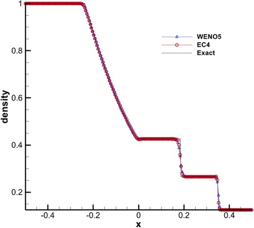
5.2. Test 2: Sod shock-tube problem

Initial condition and computing time: (47) $\begin{array}{r}\left\{\begin{array}{l}({\rho }_L,u_L,p_L)=(1,\text{0,1})\\ ({\rho }_R,u_R,p_R)=(\text{0}.12\text{5},\text{0},\text{0}.\text{1})\end{array}\right.,t=0.2\end{array}$(47) 200 points were used, CFL = 1, and s = 5 was used in EC4. The results are given in Figure 2, which shows that the resolution of EC4 was roughly equal to that of WENO5. At the same time, EC4 performed better in the case of discontinuities.

Figure 1. Results of Test 1.

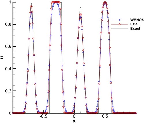
Figure 2. Results of Test 2.

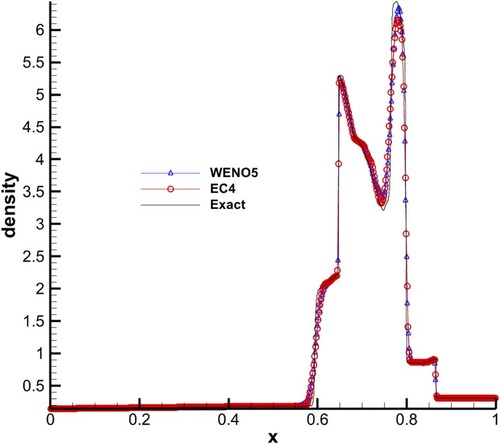
5.3. Test 3: Blast-wave problem

Initial condition and computing time: (48) $\begin{array}{rl}{\mathbf{u}}_0& =\left\{\begin{array}{l}({\rho }_L,u_L,p_L)=(1,0,1000),0\le x<0.1\\ ({\rho }_M,u_M,p_M)=(1,0,0.01),0.1\le x<0.9\\ ({\rho }_R,u_R,p_R)=(1,0,100),0.9\le x<1\end{array}\right.,\\ t& =0.038\end{array}$(48) 500 points were used (where WENO5 under the Roe formulation does not satisfy the entropy condition, and an unphysical discontinuity occurs at 500 points. Therefore, 501 points were used for replacing. Details are given in Section 6.3 ‘Sonic point tests’). CFL = 1.0 for both schemes, and s = 5 in EC4. The results are shown in Figure 3, in which it can be seen that the resolutions of the two schemes are almost the same, except that WENO5 did better at the maximum while EC4 did better at the depression.

Figure 3. Results of Test 3.

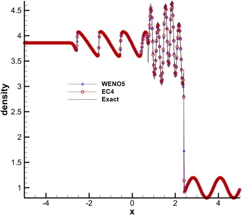
5.4. Test 4: Shu–Osher problem

Initial condition and computing time: (49) $\begin{array}{r}{\mathbf{u}}_0=\left\{\begin{array}{l}({\rho }_L,u_L,p_L)=(3.857,2.629,10.333),\\ -5\le x<-4\\ ({\rho }_R,u_R,p_R)=(1+0.2\sin 5x,0,1),\\ -4<x<5\end{array}\right.,t=1.8\end{array}$(49) 500 points were used, CFL = 1.0, set s = 5 in EC4. The results are given in Figure 4. Problems with multi-extreme points are the best tests to show the advantage of high-order schemes. In this test, the resolutions of two schemes were evenly matched, and EC4 performed better at some extremes. Considering CPU times, EC4 is superior to WENO5 (see Section 6.2 ‘CPU time tests’).

Figure 4. Results of Test 4.

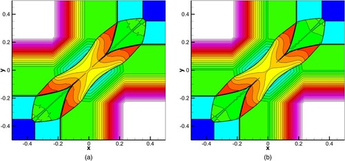
5.5. Test 5: Two-dimensional Riemann problem

Initial condition and computing time: (50) $\begin{array}{r}\left\{\begin{array}{l}\rho =1.0,p=1.0,\\ u=0,v=0& x\times y\le 0\\ \rho =0.125,p=0.1,\\ u=0,v=0& x\times y\ge 0\end{array}\right.,t=0.2\end{array}$(50) A mesh of 800 × 800 was used, CFL = 1.0, and s = 5 in EC4. The results are given in Figure 5, which shows that the overall resolutions of EC4 and WENO5 are roughly the same. EC4 performed better in some regions and WENO5 too.

Figure 5. Results of Test 5, density contours: (a) WENO5; (b) EC4.

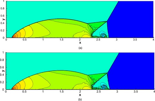
5.6. Test 6: Double Mach reflection problem

This is a classic test for investigating high-resolution schemes. The Euler equations were solved in a computational domain of (x,y) ∈ [0,4] × [0,1] and a mesh of 1600 × 400 was adopted. For EC4, s = 5 was set. The reflecting wall lay at the bottom of the computational domain starting from x = 1/6. Initially, a right-moving Mach 10 shock was positioned at x = 1/6, y = 0, making a 60° angle with the x-axis. For the bottom boundary, the exact post-shock condition was imposed for the part from x = 0 to x = 1/6 and a reflective boundary condition was used for the rest. At the top boundary of the computational domain, the flow values were set to describe the exact motion of the Mach 10 shock. More precisely, the initial condition was ρ = 1.4, p = 1.0, u = 0, v = 0 ahead of the shock, and the exact post-shock condition was imposed by the Hugoniot relation. The results are displayed at t = 0.2 (in Figure 6), which shows the resolution of EC4 was higher than that of WENO5.

Figure 6. Results of Test 6, density contours: (a) WENO5; (b) EC4.

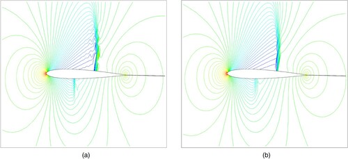
5.7. Test 7: Airfoil flow problem for NACA0012

The Mach number of free streams was Ma_∞ = 0.8, and the angle of attack was α = 1.25°. A mesh of 269 × 59 (flow direction × normal direction, 169 on wall) was used in this test, as shown in Figure 7. The coefficient of pressure on the wall computed by WENO5-RF (Roe with entropy fix) and EC4 (s = 5) are displayed in Figures 8 and 9, showing the pressure contours around the airfoil. From the results of Figures 8 and 9, it can be seen that some oscillations occur both on the upper and nether walls near the shocks, while EC4 performs well.

6. Accuracy order/efficiency/sonic point tests

Nine tests are given in this section: two accuracy order tests for scalar equations; three CPU time tests for Euler equations; and four sonic point tests for Euler equations that contain sonic points in rarefaction waves.

Figure 7. Grid around wall.

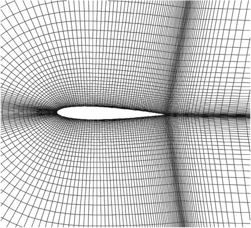
Figure 8. Pressure coefficient on wall.

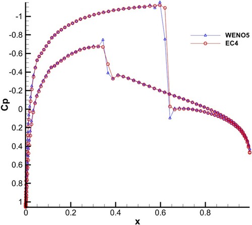
Figure 9. Pressure contours: (a) WENO5; (b) EC4.

6.1. Accuracy order test

In this section, accuracy order tests are done for linear and nonlinear cases, respectively.

6.1.1. Accuracy order test 1: Linearization equation

(51) $\begin{array}{r}\left\{\begin{array}{l}{u}_t+u_x=0,t=10\\ \\ u_0\left(x\right)=\sin \left(\pi x\right),x\in [-1,1]\end{array}\right.\end{array}$(51)

6.1.2. Accuracy order test 2: Burgers equation

(52) $\begin{array}{r}\left\{\begin{array}{l}{u}_t+{\left(\frac{u^2}{2}\right)}_x=0,t=0.15\\ \\ u_0\left(x\right)=0.5+\sin \left(\pi x\right),x\in [0,2]\end{array}\right.\end{array}$(52)

Tables 1–3 show that EC4 and WENO5 achieve their designed accuracy order. Note that the order of WENO5 in Table 4 is lower than its designed accuracy order; this is probably due to the use of the RK4 method to render its time accuracy,which doesn’t meet fifth order when CFL is not near zero.

Table 1. Error and accuracy order of EC4, Test 1.

EC4 (CFL = 0.5 s = 5)	L1 error	L1 order
grids = 20	6.363 × 10^−3
grids = 40	6.121 × 10^−4	1. 3. 378
grids = 80	4.254 × 10^−5	1. 3. 847
grids = 160	3.066 × 10^−6	1. 3. 794
grids = 320	2.087 × 10^−7	1. 3. 877
grids = 640	1.376 × 10^−8	1. 3. 923

Table 2. Error and accuracy order of WENO5, Test 1.

WENO5 (RK4, CFL = 0.5)	L1 error	L1 order
grids = 20	6.739 × 10^−3
grids = 40	2.246 × 10^−4	4.907
grids = 80	7.017 × 10^−6	5.000
grids = 160	2.200 × 10^−7	4.995
grids = 320	6.992 × 10^−9	4.975
grids = 640	2.324 × 10^−10	4.911

Table 3. Error and accuracy order of EC4, Test 2.

(A)
EC4 (CFL = 0.5 s = 5)	L1 error	L1 order
grids = 20	5.537 × 10^−4
grids = 40	6.513 × 10^−5	1. 3. 0877
grids = 80	5.831 × 10^−6	1. 3. 4815
grids = 160	5.652 × 10^−7	1. 3. 3669
grids = 320	5.194 × 10^−8	1. 3. 4438
grids = 640	4.627 × 10^−9	1. 3. 4887
(B)
EC4 (CFL = 1 s = 5)	L1 error	L1 order
grids = 20	4.783 × 10^−4
grids = 40	4.461 × 10^−5	1. 3. 4225
grids = 80	2.644 × 10^−6	1. 4. 0766
grids = 160	2.284 × 10^−7	1. 3. 5331
grids = 320	1.976 × 10^−8	1. 3. 5309
grids = 640	1.622  × 10^−9	1. 3. 6067

Note: CFL = 0.5 in (A), CFL = 1 in (B).

Table 4. Error and accuracy order of WENO5, Test 2.

(A)
WENO5 (RK4, CFL = 0.5)	L1 error	L1 order
grids = 20	4.405 × 10^−4
grids = 40	2.855 × 10^−5	1. 3. 9476
grids = 80	1.435 × 10^−6	1. 4. 3144
grids = 160	6.465 × 10^−8	1. 4. 4723
grids = 320	1.875 × 10^−9	1. 5. 1077
grids = 640	4.364 × 10^−11	1. 5. 4251
(B)
WENO5 (RK4, CFL = 1)	L1 error	L1 order
grids = 20	4.069 × 10^−4
grids = 40	2.610 × 10^−5	1. 4. 0770
grids = 80	1.554 × 10^−6	1. 4. 0700
grids = 160	8.729 × 10^−8	1. 4. 1540
grids = 320	4.125 × 10^−9	1. 4. 4034
grids = 640	2.183 × 10^−10	1. 4. 2400

Note: CFL = 0.5 in (A), CFL = 1 in (B).

6.2. CPU time test

In this subsection, two 1D Euler equations (the Sod shock-tube problem and the blast-wave problem) were chosen to test the CPU time of EC4, while reference objects were all set as WENO5-RK4. In the tests, the codes of EC4 (s = 5) and WENO5-RK4 had already been optimized.

6.2.1. CPU time test 1: Sod shock-tube problem

Table 5 shows that, with the same grids, the error of EC4 is lower than WENO5, and the CPU time of EC4 is only one third of WENO5-RK4. This demonstrates the excellent efficiency of EC4.

Solutions contain discontinuities for the tests of Tables 5 and 6, while solutions are smooth for the tests of Tables 1–4. This means that EC4 has higher resolution for discontinuities and, for smooth solutions, the accuracy order plays the main role. So, for the same grids, the error of EC4 is lower than that of WENO5 in Tables 5 and 6, but in Tables 1–4, the error of EC4 is larger than that of WENO5 on the same grids.

Table 5. Errors and CPU times of EC4 and WENO5, Sod shock-tube problem.

	L1 error			CPU time (s)
	WENO5	EC4		WENO5	EC4
grids = 10,000, CFL = 1	8.006 × 10^−5	6.198 × 10^−5		68.612	23.385
grids = 5,000, CFL = 1	1.474 × 10^−4	1.081 × 10^−4		17.233	5.757
grids = 5,000, CFL = 0.5	1.389 × 10^−4	1.209 × 10^−4		34.108	11.751

Table 6. Errors and CPU times of EC4-Baseline and WENO5, Sod shock-tube problem.

	L1 error		CPU time (s)
	WENO5	EC4-Baseline	WENO5	EC4-Baseline
grids = 10,000, CFL = 1	8.006 × 10^−5	7.351 × 10^−5	68.612	14.179
grids = 5,000, CFL = 1	1.474 × 10^−4	1.298 × 10^−4	17.233	3.542
grids = 5,000, CFL = 0.5	1.389 × 10^−4	1.321 × 10^−4	34.108	7.021

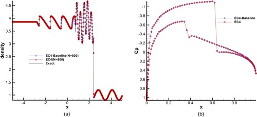
Table 6 shows that, if the flux linearization part of EC4 is performed with baseline reconstruction (with second-order nonlinear time accuracy), the CPU time of EC4-Baseline only takes nearly one-fifth that of WENO5-RK4. The practical significance lies in the following: (1) for simple unsteady problems, like the 1D problem under certain time (Figure 10(a)), EC4-Baseline can be used approximately instead of EC4 to achieve higher resolution with more points (see CPU tests 2 and 3); (2) for some steady problems, as in Section 6 test 7 in this article (the airfoil flow problem for NACA0012 shown in Figure 10(b)), EC4 can be simplified to EC4-Baseline. Then savings can be made on the time cost of the project.

Figure 10. Comparison of EC4 and EC4-Baseline: (a) density of Shu–Osher problem; (b) pressure coefficient on wall of NACA0012.

6.2.2. CPU time test 2: Shu–Osher problem

6.2.3. CPU time test 3: Blast-wave problem

Tables 7 and 8 and Figures 11 and 12 show that: (1) with almost the same CPU time, the resolution of EC4 is superior to that of WENO5, especially at the discontinuities. This is because the spatial fifth order (semi-discrete fifth order) of WENO5 is composed of three third-order weighted terms (semi-discrete third order) while no second-order or fourth-order terms exist in it. This leads to its worse performance at the discontinuities compared with EC4; (2) with almost the same CPU time, EC4-Baseline can perform with denser mesh and then achieve higher resolution.

Figure 11. CPU time test 2, Shu–Osher problem.

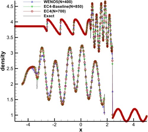
Figure 12. CPU time test 3, blast-wave problem.

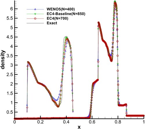
Table 7. CPU times of EC4 and WENO5, Shu–Osher problem.

	CPU time (s)
	WENO5-RK4	EC4-Baseline	EC4
grids = 400, CFL = 1	0.230	0.055	0.070
grids = 700, CFL = 1	0.689	0.150	0.230
grids = 850, CFL = 1	1.089	0.240	0.350

Table 8. CPU times of EC4 and WENO5, blast-wave problem.

	CPU time (s)
	WENO5-RK4	EC4-Baseline	EC4
grids = 400, CFL = 1	0.400	0.095	0.130
grids = 700, CFL = 1	1.208	0.259	0.420
grids = 850, CFL = 1	2.059	0.380	0.650

6.3. Sonic point tests

This subsection verifies the entropy condition satisfying property of EC4. Entropy condition violating schemes may give unphysical solution at sonic points in rarefaction waves, namely rarefaction shocks. Here s = 5 is set in EC4, and CFL = 1 for all the following tests.

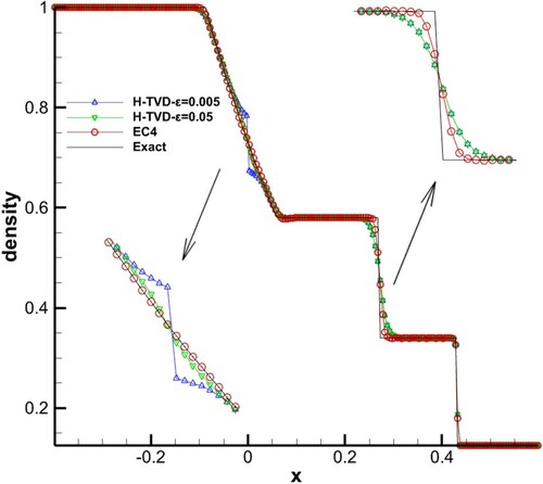
6.3.1. Sonic point test 1: Modified Sod problem

The modified Sod problem (Toro, 2009), which contains a sonic point in the rarefaction wave, was tested as follows. The second-order Harten–TVD (Total Variation Diminishing) (Harten, 1983) scheme was set as the comparison. It uses an entropy fix function Q(ν) to avoid unphysical solutions. The initial condition and computing time are given as follows: (53) $\begin{array}{r}\left\{\begin{array}{l}({\rho }_L,u_L,p_L)=(1,0.75,1)\\ ({\rho }_R,u_R,p_R)=(0.125,0,0.1)\end{array}\right.,t=0.2\end{array}$(53) 200 points were used. The entropy fix function Q(ν) of the Harten–TVD scheme is equal to adding an artificial numerical viscosity at the sonic point. Q(ν) is given as follows: (54) $\begin{array}{r}Q\left(\nu \right)\equiv \left\{\begin{array}{l}|\nu ||\nu |>ϵ\\ \\ \frac{{\nu }^2+{ϵ}^2}{2ϵ}|\nu |\le ϵ\end{array}\right.\end{array}$(54) where ν = aτ/h is a dimensionless eigenvalue. When ν = 0, the numerical viscosity vanishes, if this happens in a rarefaction wave, false discontinuities may appear, so Harten used a small artificial viscosity such as ε = 0.005∼0.05 to avoid it. This method is called an entropy fix.

In Figure 13, H-TVD means the second-order Harten–TVD scheme, and EC4 means the fourth-order entropy condition scheme. From Figure 13 we notice that, when the extra numerical viscosity is insufficient at the sonic point (such as when ε = 0.005), H-TVD still obtains an unphysical discontinuity. However, EC4 can meet the entropy condition without an extra numerical viscosity.

Figure 13. Sonic point test 1, modified Sod problem.

6.3.2. Sonic point test 2: Blast-wave problem

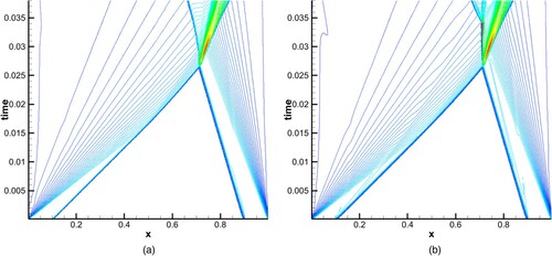
Four grid number groups were set that contain 500, 501, 599 and 600 points to test EC4 and WENO5, respectively. The initial condition and computing time were as for (48).

WENO5-RK4 with the Roe formulation does not satisfy the entropy condition, which leads to the possibility of unphysical discontinuities occurring. Figure 14 shows that a false discontinuity is produced by WENO5 in grid numbers 500 and 600, and it vanishes if replaced with 501 and 599 points (nearby values), respectively, while EC4 has no unphysical discontinuity in any case.

This anomalous phenomenon of WENO5 has not been found in the literature. In order to investigate why it is so, the blast-wave problem was simplified and Sonic point test 3 constructed where WENO5 holds in the anomalous phenomenon such that the false discontinuity sometimes appears and sometimes does not appear for different grid numbers. The test was simplified further as design Sonic point test 4, and this time WENO5’s false discontinuity was fixed no matter what the grid number.

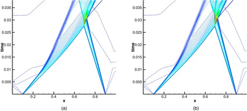
Following Figures 14 and 15, it can be seen that the false discontinuity appears at the intersection of multiwaves, and there seems to be a static shock wave just after the intersection of two shocks on a rarefaction wave in Figure 15. Therefore, it is speculated that the static shock provides a discontinuity with zero eigenvalue (sonic point), and the rarefaction wave provides an expansion field. When they coincide instantaneously, a static ‘expansion discontinuity’ is formed, which, if it is captured by numerical solutions, schemes that do not satisfy the entropy condition may develop false discontinuities. According to this analysis, the following test was designed.

Figure 14. Sonic point test 2, blast-wave problem.

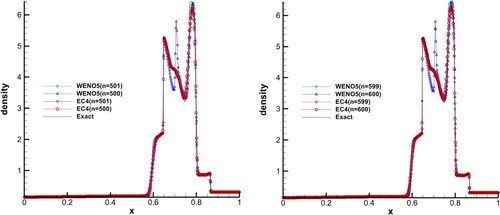
Figure 15. Density contours of blast-wave problem in the x–t plane for 500 points: (a) EC4; (b) WENO5.

6.2.3. Sonic point test 3: Simplified blast-wave problem

The initial value of the blast-wave problem was modified to make two rarefaction waves and two shocks intersect at (x, t) = (223/310, 8/310), and it also produced a contact discontinuity, see Figure 16(a). In this test, reflection boundaries were applied at both ends, 310 points were used, and the false discontinuity can be found at point No. 223. The initial condition and computing time were as given below: (55) $\begin{array}{rl}{\mathbf{u}}_0& =\left\{\begin{array}{l}({\rho }_L,u_L,p_L)\\ =(5.9993,20,480),& 0\le x<0.1\\ ({\rho }_M,u_M,p_M)\\ =(1,0,0.01),& 0.1\le x<0.9\\ ({\rho }_R,u_R,p_R)\\ =(5.9914,-5.8317,40.832),& 0.9\le x<1\end{array}\right.,\\ t& =0.038\end{array}$(55) According to Figures 16(b) and 17, for WENO5, a false discontinuity is formed at the position of multiwave intersection (the grid position set above), and there is also a static shock wave, while EC4 meets the entropy condition, and no unphysical discontinuity appears. At the same time, the phenomenon is in line with Sonic point test 2 if we use different grid numbers, which proves the randomness correlation of grid numbers of WENO5.

Figure 16. Sonic point test 3, simplified blast-wave problem: (a) construction of Sonic point test 3; (b) density of Sonic point test 3.

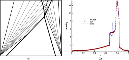
Figure 17. Density contours of simplified blast-wave problem in the x–t plane: (a) EC4; (b) WENO5.

The randomness of results related to grid numbers may be because: (1) before the intersection, shocks are not static; (2) after the intersection, shocks are quickly bent by rarefaction waves; and (3) the static shock has only a transient existence. If the transient static shock can be captured by WENO5, false discontinuity appears, otherwise no false discontinuities appear. Meanwhile, the contact discontinuity formed after the intersection of waves is also a possible instability factor that may cause solution overleaping. To eliminate the possibility of the instability phenomenon due to singularity superposition, it is hoped to construct an example with a simple wave structure to verify whether the above phenomenon is caused by static shock waves. That is to say, what is needed is a simple case without contract discontinuity or the appearance of false discontinuity without grid randomness. Therefore, perhaps intersecting two simple waves would be a good method. According to the above analysis, the test is revised once more as follows.

6.2.4. Sonic point test 4: Intersection of rarefaction wave and static shock

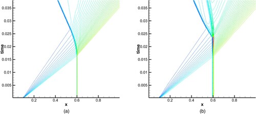
Let a rarefaction wave intersect with a static shock of a different family. In addition to the waves crossing each other, an entropy wave will also be generated, see the dotted line in Figure 18(a). Here, constant boundaries were applied at both ends and 200 points were used. The initial condition and computing time were as given below: (56) $\begin{array}{rl}{\mathbf{u}}_0& =\left\{\begin{array}{ll}({\rho }_L,u_L,p_L)=(1.6583,8,79.317),& 0\le x<0.1\\ ({\rho }_M,u_M,p_M)=(6,20,480),& 0.1\le x<0.6\\ ({\rho }_R,u_R,p_R)=(15,8,1920),& 0.6\le x<1\end{array}\right.,\\ t& =0.038\end{array}$(56) Numerical experiments showed this test enabled WENO5 to produce a false discontinuity at the first intersection. Figures 18(b) and 19 show that WENO5 produces a false discontinuity at the position where the rarefaction wave and the static shock wave intersect. Moreover, in this test, WENO5 will have false discontinuities at arbitrary grid numbers, while there will be none in EC4.

Figure 18. Sonic point test 4, intersection of rarefaction wave and static shock: (a) construction of Sonic point test 4; (b) density of Sonic point test 4.

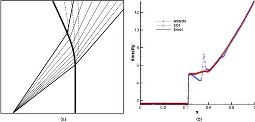
Figure 19. Density contours of intersection of rarefaction wave and static shock in the x–t plane: (a) EC4; (b) WENO5.

6.2.5. Summary of sonic point tests

By Sonic point tests 2, 3 and 4, it can be concluded that, for schemes not meeting the entropy condition, such as WENO5-Roe, when a static shock wave is formed by the intersection of waves, although the rarefaction wave will bend it soon, if the scheme can capture the instantaneous static shock at some grid numbers, there will be a false discontinuity; if not, it will not appear. This explains the randomness correlation of grid numbers in Sonic point tests 2 and 3. While for Sonic point test 4, the intersection of rarefaction and static shock waves makes the static shock wave fixed on the grid, so the randomness disappears thereupon. These four tests fully reflect the entropy condition satisfying property of EC4.

7. Conclusions

Different from RK-WENO schemes based on semi-discrete ones with the Runge–Kutta method, this article proposes a fully-discrete non-oscillatory scheme. Different from the LW-WENO scheme based on a Lax–Wendroff type process and the ADER scheme based on a Godunov type process, this article proposes a fully-discrete scheme based on a solution formula method. On the basis of Dong et al. (2002), a fourth-order entropy condition scheme (EC4) is given through accuracy order analysis of a general form of entropy condition scheme and the meticulous design of limiters and smoothness thresholds. EC4 possesses the following advantages: (1) it is fully-discrete, has fourth-order accuracy in time and space uniformly, is stable with one step when CFL = 1, and without Runge–Kutta processes; (2) it achieves both high resolution and robustness (WENO-Roe achieves high resolution but sometimes loses robustness, WENO-LLF achieves robustness but sometimes loses resolution); (3) it is simple and compact with seven points, which meets the requirement of replacing the traditional second-order schemes in industry applications; (4) it satisfies the entropy condition, which has been confirmed by the numerical experiments; (5) it is qualified by its high efficiency. For problems where the discontinuities are dominant, using the same grid, the error of EC4 is less than that of WENO5-RK4, and the CPU time of EC4 is only one third of that of WENO5-RK4. For problems where fine structures are dominant, EC4 can perform with a denser grid and achieve higher resolution than WENO5-RK4 within the same CPU time. Overall, the efficiency of the new scheme is superior to that of WENO5; (6) this article does not provide a comparison with other schemes, but it can be compared indirectly by means of the literature: the efficiency improvement over RK-WENO by the LW-WENO scheme or the ADER scheme is no more than twice; however, the improvement can be three to four times with EC4 (EC4-Baseline even achieves nearly five times).

Future expectations: the entropy condition (EC) schemes based on the solution formula method are equipped with high value both in theory and engineering application. So the EC scheme and the solution formula method are valuable and significant research directions. We have proposed EC4, but this is just the beginning. The limitation of this study is that the non-oscillatory condition in this article is only for fourth-order schemes, no law has been obtained for higher-order schemes. In this latest study towards higher-order schemes, although higher accuracy order has indeed been obtained, robustness has not been guaranteed; perhaps some other techniques need to be considered. It is also hoped to find an optimization method to ensure that the smooth threshold s can be slightly magnified as well as the non-oscillatory property obtained. Next, the current authors are preparing to construct higher-order, one-step, fully-discrete schemes and to transform the existing high-order, semi-discrete schemes (such as WENO) into one-step, fully-discrete ones by this method.

Disclosure statement

No potential conflict of interest was reported by the authors.

References

- Ben-Artzi, M., & Falcovitz, J. (1984). A second-order Godunov-type scheme for compressible fluid dynamics. Journal of Computational Physics, 55(1), 1–32. https://doi.org/https://doi.org/10.1016/0021-9991(84)90013-5
- Deng, X., & Zhang, H. X. (2000). Developing high-order weighted compact nonlinear schemes. Journal of Computational Physics, 165(1), 22–44. https://doi.org/https://doi.org/10.1006/jcph.2000.6594
- Dong, H. T. (2000). (Mm)∞ operators and viscosity solutions for Hamilton-Jacobi equations. Pure and Applied Mathematics, 16(4), 64–75.
- Dong, H. T., Zhang, L. D., & Lee, C. H. (2002). High order discontinuities decomposition entropy condition schemes for Euler equations. CFD Journal, 10(4), 563–568.
- Du, Z., & Li, J. (2018). A Hermite WENO reconstruction for fourth order temporal accurate schemes based on the GRP solver for hyperbolic conservation laws. Journal of Computational Physics, 355, 385–396. https://doi.org/https://doi.org/10.1016/j.jcp.2017.11.023
- Fu, D., & Ma, Y. (1997). A high order accurate difference scheme for complex flow fields. Journal of Computational Physics, 134(1), 1–15. https://doi.org/https://doi.org/10.1006/jcph.1996.5492
- Ghalandari, M., Bornassi, S., Shamshirband, S., Mosavi, A., & Chau, K. W. (2019). Investigation of submerged structures’ flexibility on sloshing frequency using a boundary element method and finite element analysis. Engineering Applications of Computational Fluid Mechanics, 13(1), 519–528. https://doi.org/https://doi.org/10.1080/19942060.2019.1619197
- Harten, A. (1983). High resolution schemes for hyperbolic conservation laws. Journal of Computational Physics, 49(3), 357–393. https://doi.org/https://doi.org/10.1016/0021-9991(83)90136-5
- Harten, A., Engquist, B., Osher, S., & Chakravarthy, S. (1987). Uniformly high order accurate essentially non-oscillatory schemes, III. Journal of Computational Physics, 71(2), 231–303. https://doi.org/https://doi.org/10.1016/0021-9991(87)90031-3
- Lax, P. D. (1973). Hyperbolic systems of conservation laws and the mathematical theory of shock waves. SIAM Reg. Conf. Series, Lectures in Applied Math, 11, 1–48. https://doi.org/https://doi.org/10.1137/1.9781611970562.fm
- Lax, P. D., & Wendroff, B. (1960). Systems of conservation laws. Communications on Pure and Applied Mathematics, 13(2), 217–237. https://doi.org/https://doi.org/10.1002/cpa.3160130205
- Lele, S. K. (1992). Compact finite difference schemes with spectral-like resolution. Journal of Computational Physics, 103(1), 16–42. https://doi.org/https://doi.org/10.1016/0021-9991(92)90324-R
- Li, J., & Du, Z. (2016). A two-stage fourth order time-accurate discretization for Lax–Wendroff type flow solvers, I: Hyperbolic conservation laws. SIAM Journal on Scientific Computing, 38(5), A3046–A3069. https://doi.org/https://doi.org/10.1137/15M1052512
- Liu, S., & Shen, Y. (2020). Two-step weighting method for constructing fourth-order hybrid central WENO scheme. Computers & Fluids, 207, 104590. https://doi.org/https://doi.org/10.1016/j.compfluid.2020.104590
- Liu, X. D., Osher, S., & Chan, T. (1994). Weighted essentially non-oscillatory schemes. Journal of Computational Physics, 115(1), 200–212. https://doi.org/https://doi.org/10.1006/jcph.1994.1187
- Peng, J., & Shen, Y. (2015). Improvement of weighted compact scheme with multi-step strategy for supersonic compressible flow. Computers & Fluids, 115, 243–255. https://doi.org/https://doi.org/10.1016/j.compfluid.2015.04.012
- Qiu, J., & Shu, C. W. (2003). Finite difference WENO schemes with Lax-Wendroff-type time discretizations. SIAM Journal on Scientific Computing, 24(6), 2185–2198. https://doi.org/https://doi.org/10.1137/S1064827502412504
- Roe, P. L. (1981). Approximate Riemann solvers, parameter vectors, and difference schemes. Journal of Computational Physics, 43(2), 357–372. https://doi.org/https://doi.org/10.1016/0021-9991(81)90128-5
- Salih, S. Q., Aldlemy, M. S., Rasani, M. R., Ariffin, A. K., Ya, T. M. Y. S. T., Al-Ansari, N., Yaseen, Z. M., & Chau, K.-W. (2019). Thin and sharp edges bodies-fluid interaction simulation using cut-cell immersed boundary method. Engineering Applications of Computational Fluid Mechanics, 13(1), 860–877. https://doi.org/https://doi.org/10.1080/19942060.2019.1652209
- Shen, Y., Liu, L., & Yang, Y. (2014). Multistep weighted essentially non-oscillatory scheme. International Journal for Numerical Methods in Fluids, 75(4), 231–249. https://doi.org/https://doi.org/10.1002/fld.3889
- Sod, G. A. (1978). A survey of several finite difference methods for systems of nonlinear hyperbolic conservation laws. Journal of Computational Physics, 27(1), 1–31. https://doi.org/https://doi.org/10.1016/0021-9991(78)90023-2
- Strang, G. (1968). On the construction and comparison of difference schemes. SIAM Journal on Numerical Analysis, 5(3), 506–517. https://doi.org/https://doi.org/10.1137/0705041
- Titarev, V. A., & Toro, E. F. (2002). ADER: Arbitrary high order Godunov approach. Journal of Scientific Computing, 17(1/4), 609–618. https://doi.org/https://doi.org/10.1023/A:1015126814947
- Toro, E. F. (2009). Riemann solvers and numerical methods for fluid dynamics (3rd ed. pp. 225–226). Springer.
- Toro, E. F., & Titarev, V. A. (2006). Derivative Riemann solvers for systems of conservation laws and ADER methods. Journal of Computational Physics, 212(1), 150–165. https://doi.org/https://doi.org/10.1016/j.jcp.2005.06.018
- Tveit, S. (2011). Numerical methods for conservation laws with a discontinuous flux function. VDP Technology Rock & Petroleum Disciplines.