Simulation strategy of the full-scale ship resistance and propulsion performance

Abstract

The ship powering performance can be predicted based on model tests or simulations. However, differences exist between the full-scale ship performance and extrapolated model data. Therefore, research on full-scale ship performance simulation has important scientific significance and engineering value. This study used the REGAL general cargo vessel to perform full-scale ship resistance and self-propulsion simulations for various grid numbers, time step sizes, and wall Y+ values and compared the calculation and empirical results. The resistance components, waveform, Courant–Friedrichs Lewy (CFL) number, pressure field, and wake flow field of various resistance simulation conditions were analysed. The wall Y+ value was observed to affect the capture of boundary layer flow, ship pressure field evolution, and waveform, which subsequently affect the ship resistance. A Y+ value within 200 was considered to be appropriate when simulating the powering performance of a full-scale ship. The waveform evolution was significantly affected by the time step size, which should meet the requirement that the CFL number on the free surface is less than 1. When simulating the self-propulsion of a full-scale ship based on sliding mesh, the CFL number on the interface should also be less than 1. Additionally, to obtain the correct propeller excitation force, it was recommended that the time step size be maintained below 1°/step (0.000076 L_PP/v).

KEYWORDS:

• Full-scale simulation
• time step size
• ship resistance
• CFD
• propulsion performance
• excitation force

1. Introduction

Presently, model scale tests and simulations are used for predicting and optimising the design of a ship, which ensures optimal powering performance. However, the scale effect causes a large error in the process of converting the model test data for the difference in the Reynolds number (Raven et al., 2008). Although there are empirical formulas that can be used to correct this error, serious problems concerning the wake adapted propeller design (Wang et al., 2017, 2018) and energy-saving effect analysis for the energy-saving device exist (Song et al., 2020; Koushan et al., 2020). With the recent developments in computer software, hardware technology, and numerical simulation methods for fluid mechanics (Salih et al., 2019; Su et al., 2019), the powering performance of full-scale ships, which is based on computation fluid dynamics (CFD), is being actively researched.

The calculation of the powering performance of full-scale ships can be roughly divided into the following parts. These parts include the ship resistance and wake field, the ship self-propulsion, predicting the effect of energy-saving devices, and the seakeeping performance of the ship.

For the simulation of the full-scale ship resistance and the wake field, since 2005, researchers have performed full-scale viscous flow calculations based on the ‘European Union Project EFFORT’ (Visonneau, 2005; Visonneau et al., 2006). Tahara (2002) considered simultaneously the effect of the surface roughness to carry out a numerical study on the series 60 ship. They demonstrated that the wall function in combination with the roughness model can initially simulate the effect of the ship surface roughness. Hochkirch and Mallol (2013) identified the differences among different scaled ships with respect to wake field, stern wave breaking, and energy-saving device benefits. In addition, they described the necessity of calculating the powering performance of the full-scale ship. Based on the 4000TEU container ship, Wang et al. (2015) carried out a numerical solution of the nominal wake field for various scales and proposed a method for extrapolating the wake field based on the model data.

Zhang et al. (2018) performed the full-scale resistance simulation of DTMB5415; the difference between the simulated resistance value and extrapolated value was 5.63%. Song et al. (2019) predicted the impact of biofouling based on the rough wall function. The results demonstrated that the frictional resistance of the ships at the design speed (24 knots) and low speed (19 knots) increased by 93 and 88%, respectively. Sun et al. (2019) calculated the wake field of a full-scale four-propeller full appendage ship, which has complicated appendages such as shafting, bracket, and deadwood in the stern compared with single propeller propulsion. In addition, the wake field is considerably affected by the appendages, which indicates a more complex scale effect law. By considering the KCS and KVLCC2 as their research objects, Dogrul et al. (2020) analysed the scale effect on ship resistance component and the characteristics of the flow field. With the increase in the Reynolds number, the residual resistance coefficient of the KCS remained unchanged for all scales, whereas that of the KVLCC2 displayed a downward trend. This is due to the different scale effects of the frictional and wave-making resistances, along with the different proportions of the resistance components of the two ships.

In terms of full-scale ship self-propulsion simulations, Castro et al. (2011) performed self-propulsion calculations on KCS based on the dynamic overlapping grids method. In addition, they discussed the differences in the navigation performance of the two scale ships and provided a rationale for the differences from the perspective of the flow field. Bhushan et al. (2007, 2009) performed a numerical study on the powering performance of the full-scale Athena and DTMB5415 ships. It was determined that a simulation that considers the rough wall offers a more accurate prediction of the frictional resistance and the total resistance, which is closer to the extrapolation results of the test. Based on the detached-eddy simulation (DES) model, Ponkratov (2015) of Lloyd's Register (LR) carried out a full-scale propeller cavitation simulation. In comparison to the ship observation results, the sheet cavitation was well simulated; however, the tip vortex cavitation was not reproduced well. Ponkratov and Zegos (2015) conducted a full-scale ship self-propulsion simulation using the commercial software STAR-CCM+, and compared the CFD forecast results with the International Towing Tank Conference (ITTC) forecast methods and the sea trial measurement results. Farkas et al. (2018) carried out a systematic analysis to predict the powering performance of ships. Their analysis showed that the resistance predicted by the Reynolds stress model is the closest to the extrapolated value of the model test; however, the model required more time for simulation. In addition, the difference between the prediction results for the different extrapolation methods was greater than the influence of the turbulence model. Jasak et al. (2019) used OpenFOAM platform and virtual disk model to calculate two full-scale ships. Based on the sea trial measurement results, the grid sensitivity was verified. Sun et al. (2020) conducted full-scale ship self-propulsion simulations and analysed the influence of the scale effect on the hull–propeller interaction. Kok et al. (2020) used DTC container ships as their research object and numerically analysed the scale effect of the ship heave in shallow water. Their simulation results demonstrated that the heave of the ship is proportional to the scale ratio, and the scale effect can be ignored.

A full-scale numerical simulation aids in predicting the performance of energy-saving devices; moreover, it reveals their energy-saving mechanisms. Kawamura et al. (2012) researched and analysed the scale effect of the propeller boss cap fin (PBCF). Their results demonstrated that during the interaction of Reynolds number and wake field, the energy-saving benefit under full scale is higher than that under model scale. Hasselaar and Xing-Kaeding (2017) studied the energy-saving effect of fins on of a 52000-bulk carrier using experiments and numerical analysis. The energy-saving benefits, which can reach over 5%, obtained by experiment and numerical calculations were in good agreement. Moreover, the improvement of the hub vortex cavitation resulting from the fins was observed in the numerical calculation. Saydam et al. (2018) conducted a parametric modeling study of a vortex generator. The results showed that a reasonably designed vortex generator can significantly improve the inhomogeneity of the wake, thereby reducing the hull vibration. By analysing the ship resistance and flow field characteristics before and after the installing the stern flap, Song et al. (2020) summarised the drag reduction effect and the scale effect of the stern flap.

For the simulations of the full-scale ship seakeeping behavior, Tezdogan et al. (2015, 2016) studied the motion responses of the KCS ship using overlapping grid technology. The response characteristics of pitching and heave motions under different water depths were analysed, and the calculated results were found to be in good agreement with the experimental ones. Kim et al. (2017) performed a full-scale simulation of the modified bow form based on the KVLCC2. Their research results demonstrated that the newly designed hull form has a better performance for all of the wave length conditions, and 8% energy savings can be achieved in the five sea state conditions. Niklas and Pruszko (2019) performed full-scale ship simulations that simulated calm water and waves. In addition, they studied the effect of bow form on the ship motion response.

In summary, there has been gradual development in the powering performance calculation of full-scale ships (Lu et al., 2020). The LR Ship Performance Group organised a full-scale hydrodynamics workshop in 2016 (Lloyd's Register, 2016). However, no relevant studies have been conducted on the simulation strategy of powering performance of full-scale ships, especially for the key issues of full-scale simulations such as the time step size and the wall Y+ value. Therefore, we considered the general cargo vessel REGAL to be the research object in this study, and the full-scale ship resistance simulation strategy was constructed with the calculation analysis of various grid numbers, time step sizes, and wall Y+ values. On this basis, the self-propulsion characteristics for the various time step sizes were simulated, which were verified by comparing the results of the sea trial (Lloyd's Register, 2016). Finally, the unsteady propeller thrust and torque under the various time step sizes were analysed, and the full-scale ship self-propulsion simulation strategies under the different requirements are summarised.

2. Numerical model and approach

This section focuses on the RANS approach, turbulence model, free surface and wall treatment, computational domain, and related mesh generation used in the numerical simulations of this study.

2.1. RANS approach

The full-scale ship resistance and self-propulsion numerical simulations were carried out using the CFD software STAR-CCM+ (version 14.02), which uses Reynolds-averaged Navier–Stokes (RANS) equations: (1) $\begin{array}{rl}& \frac{\mathrm{\partial }\rho }{\mathrm{\partial }t}+\frac{\mathrm{\partial }(\rho u_i)}{\mathrm{\partial }{x}_i}=0\end{array}$(1) (2) $\begin{array}{rl}& \frac{\mathrm{\partial }(\rho u_i)}{\mathrm{\partial }t}+\frac{\mathrm{\partial }}{\mathrm{\partial }{x}_j}(\rho u_i{u}_j)\\ & =-\frac{\mathrm{\partial }p}{\mathrm{\partial }{x}_j}+\frac{\mathrm{\partial }}{\mathrm{\partial }{x}_j}\mu \left(\frac{\mathrm{\partial }{u}_i}{\mathrm{\partial }{x}_j}-\rho \overline{u_i^{\mathrm{\prime }}{u}_j^{\mathrm{\prime }}}\right)+S_j\end{array}$(2) where $\rho$ is the fluid density, $u_i$ and $u_j$ are the time-averaged values (i, j=1, 2, 3) of the velocity component, p is the pressure, $\mu$ is the dynamic viscosity coefficient, and $S_j$ is the source term.

The finite volume method (FVM) was used to discretize the computational domain, and the implicit unsteady solver was used to solve the non-uniform flow field around the ship. The governing equations were solved using a second-order upwind convection scheme and a first-order temporal discretization, and the SIMPLE algorithm for pressure–velocity coupling was used. Considering the influence of the wall shear force, the SST k-ω model was adopted as the turbulence model to simulate the flow field with strong inverse pressure gradients.

2.2. Turbulence model

The SST k-ω model is advantageous in terms of calculation of viscous flow field and the solution of flow separation. The transport equations for the turbulent kinetic energy (k) and turbulence dissipation rate (ω), respectively, are expressed as, (3) $\begin{array}{rl}\frac{\mathrm{\partial }k}{\mathrm{\partial }t}+\overline{u_j}\frac{\mathrm{\partial }k}{\mathrm{\partial }{x}_j}& =\frac{\mathrm{\partial }}{\mathrm{\partial }{x}_j}[(\nu +{\sigma }_k\nu )\frac{\mathrm{\partial }k}{\mathrm{\partial }{x}_j}+\widetilde{P_k}-{\beta }^{\ast }k\omega ]\end{array}$(3) (4) $\begin{array}{rl}\frac{\mathrm{\partial }\omega }{\mathrm{\partial }t}+\overline{u_j}\frac{\mathrm{\partial }\omega }{\mathrm{\partial }{x}_j}& =\frac{\mathrm{\partial }}{\mathrm{\partial }{x}_j}[(\nu +{\sigma }_{\omega }\nu )\frac{\mathrm{\partial }\omega }{\mathrm{\partial }{x}_j}+\alpha S^2-\beta {\omega }^2\\ & +2(1-F_1){\sigma }_{\omega 2}\frac{1}{\omega }\frac{\mathrm{\partial }k}{\mathrm{\partial }{x}_j}\frac{\mathrm{\partial }\omega }{\mathrm{\partial }{x}_j}]\end{array}$(4) The eddy-viscosity coefficient is expressed as $v_t=\frac{a_{1}k}{max(a_1\omega ,\mathrm{\Omega }{F}_2)}$ where ${\sigma }_k=\frac{1}{F_1/{\sigma }_{k,1}+(1-F_1)/{\sigma }_{k,2}}$ and ${\sigma }_{\omega }=\frac{1}{F_1/{\sigma }_{\omega ,1}+(1-F_1)/{\sigma }_{\omega ,2}}$

The definition of blending functions F1 and F2 is as follows (5) $F_1=\tanh ({\mathrm{\Phi }}_1^4)$(5) (6) $F_2=\tanh ({\mathrm{\Phi }}_2^2)$(6) where

The constant coefficients $\phi$ in the aforementioned equations (k) and (ω) are calculated by (7) $\phi ={\phi }_1{F}_1+{\phi }_2(1-F_2)$(7)

2.3. Treatment of free surface and wall

The effect of the free surface is considered in the calculation of ship resistance and self-propulsion. In this study, the volume of fluid (VOF) model is used to deal with the interface between the water and air phases. This is an accurate interface tracking method and can well simulate the free surface. The all-Y+ wall treatment method was adopted in this research, which is one of three near-wall treatment methods provided by the software STAR-CCM+. It is a hybrid near-wall treatment method, which can adjust the near-wall treatment method according to the size of Y+ (low or high).

2.4. General cargo vessel REGAL

In October 2015, LR obtained a comprehensive set of trial data using the voyage of general cargo vessels from Istanbul to Varna. In 2016, LR Ship Performance Group organised a full-scale hydrodynamics workshop (Lloyd's Register, 2016) and published the complete trial data of the REGAL.

Figure 1 shows the test and simulation model of the REGAL, which is a single-propeller propulsion ship with a mast and superstructure above the deck. According to the recommendation of the workshop, the influence of the superstructure was considered in the simulation of this study, and the mast was omitted. The parameters of the general cargo vessel REGAL and the sea trial conditions are given in Table 1.

Figure 1. Test and simulation geometry model of general cargo vessel REGAL

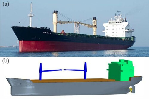
Table 1. Parameters of general cargo vessel REGAL and the sea trial conditions.

Main dimensions	Symbols	Values
Length between perpendiculars	LPP (m)	138
Breadth moulded	B (m)	23
Depth moulded	T (m)	12.1
Wetted surface	S (m^2)	3727
Displacement	▽(m^3)	12754
Service speed	V (kn)	14
Propeller diameter	D (m)	5.2
No. of blades	Z	4
Water density	ρw (kg/m^3)	1010
Air density	ρa (kg/m^3)	1.1649
Kinematic viscosity of water	vw (m^2/s)	8.8394×10^−7
Kinematic viscosity of air	va (m^2/s)	1.6036×10^−5

2.5. Computational domains and boundary conditions

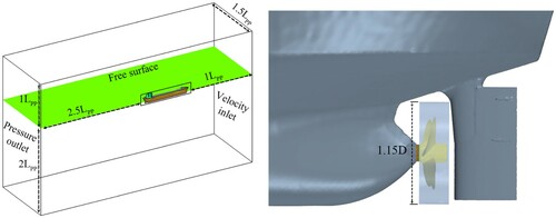
As shown in Figure 2, the resistance simulation was carried out for half of the ship by considering the symmetry of the hull. The computational domain of the ship resistance calculation is a rectangle, and its length, width, and height are 4.5L_PP × 1. 5L_PP × 3L_PP, respectively. The distance from the ship to the inlet and top of the domain is 1, 1.5 L_PP from the side, 2 L_PP from the bottom, and 2.5 L_PP from the outlet. The inlet and outlet of the computational domain were set as velocity inlet and pressure outlet, respectively, and the side was set as the symmetrical plane. To compare with the workshop results, the hull and propeller surfaces were set as smooth walls. In the self-propulsion simulations, the entire ship was modeled, and the width of the computational domain was twice that of the resistance simulation domain. As shown in Figure 2, the propeller rotation was achieved with a sliding mesh (Wang et al., 2019, 2020), and the diameter of the rotating domain was 1.15D.

Figure 2. Resistance simulation domain (left) and the propeller domain (right).

2.6. Mesh generation

The grid generator of STAR-CCM+ was used to divide the mesh of the computational domain. To improve the accuracy of the numerical simulation, it is necessary to refine specific areas of the computational domain. Figure 3 shows the grid structure of key parts of the simulation domain. It can be seen that the mesh of the free surface is refined to better simulate the free surface. Simultaneously, the bow, stern, propeller, and other areas with large surface curvature change were also refined. The mesh parameters used in the resistance (Grid G1) and self-propulsion calculations are listed inTable 2.

Figure 3. Mesh distribution: (a) Kelvin wave system, (b) bow, (c) boundary layer, (d) propeller.

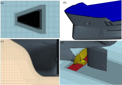
Table 2. Mesh parameters for the different working conditions.

	Number of ship boundary layers	Number of propeller boundary layers	Ship boundary layer stretching	Propeller boundary layer stretching	Background domain	Propeller domain	Total
Resistance test	14	—	1.2	—	10.99 M	—	10.99 M
Self-propulsion test	14	12	1.2	1.1	28.78 M	1.44 M	30.22 M

3. Resistance simulations

The full-scale ship resistance simulation was performed based on the REGAL. The simulation focused on the influence of the mesh numbers, time step sizes, and wall Y+ values to obtain the simulation strategy. The simulated ship speed was 14 knots, and the corresponding Froude number was 0.196. Before predicting the resistance of the multiple working conditions, the trim and sinkage were predicted, and the vertical movement and ship rotation around the Y axis were allowed in the calculation. In the subsequent multi-condition resistance calculations, the ship was pre-adjusted to the above-mentioned attitude prediction results, and then the resistance calculations of the fixed attitude were performed. On the one hand, the possible attitude difference can be avoided under different working conditions, and then the single-variable analysis of Y + and time step size can be affected. On the other hand, accelerated convergence and reduced prediction time can be achieved. The predicted trim and sinkage were 0.0344° and 0.194 m, respectively, which are consistent with the workshop results. The resistance calculation conditions are listed in Table 3.

Table 3. Resistance simulation conditions.

Item	Wall Y+	Time step size	Mesh number
Mesh uncertainty analysis	100	0.0025LPP/v	10.99M, 7.53M, 5.19M
Setting the time step size	100	0.00125LPP/v, 0.0025LPP/v, 0.005LPP/v, 0.01 LPP/v	10.99M
Selecting the wall Y+ value	60, 100, 200, 300, 500, 800	0.0025LPP/v	9.27–11.02M

3.1. Mesh uncertainty analysis

The method discussed by Stern et al. (2001) and Xing and Stern (2010) was adopted for the mesh uncertainty analysis. The Cartesian cut-cell method was used to generate the computational grids, which are composed of the prism layer mesh and trimmed mesh. To eliminate the influence of the Y+ value, keeping the topological form of the prism layer mesh unchanged when performing the mesh uncertainty analysis is necessary. The mesh refinement ratio, r, was set to 1.2. The convergence ratio$R_G$can be expressed as follows: (8) $R_G=\left|\frac{S_1-S_2}{S_2-S_3}\right|.$(8) where $S_1$,$S_2$, and $S_3$are the simulation results that correspond to the G1 (The grid parameters are given in Table 2), G2, and G3 meshes, respectively.

Based on the same mesh topology, three sets of meshes were generated by adjusting the basic parameters of the trimmed mesh. The three sets of grid parameters and the CPU simulation times are listed in Table 4.

Table 4. Mesh parameters and CPU times for the resistance simulations.

	G1 (Fine)	G2 (Medium)	G3 (Coarse)
Number of cells	10.99M	7.53M	5.19M
Number of cores	32	16	16
CPU time (h)	36	42	30

In Lloyd's Register (2016), most of the given time step sizes were distributed in the range of 0.0025–0.01 L_PP/v. The range statistics of Y+ values are given in Table 5. Based on this, a relatively small time step and Y+ value were selected in the grid uncertainty study, which are 0.0025 L_PP/v and 100, respectively.

Table 5. Choice of Y+ in Lloyd's workshop.

Range of Y+	<1	30–200	200–500	>500
Number of cases	2	5	7	4

The estimated order of accuracy$P_{RE}$ is calculated by: (9) $P_{RE}=\ln (|S_2-S_3|/|S_1-S_2|)/\ln (r).$(9) The distance metric to the asymmetric range $P_G$ is calculated by: (10) $P_G=P_{RE}/P_{th},$(10) Here, $P_{th}$ is the theoretical order of the accuracy.

The mesh uncertainty is expressed as follows: (11) $U_G=\{\begin{array}{l}(2.45-0.85P_G)\left|\frac{S_1-S_2}{r^{P_{RE}}-1}\right|,0<P_G\le 1\\ (16.4P_G-14.8)\left|\frac{S_1-S_2}{r^{P_{RE}}-1}\right|,P_G>1\end{array}$(11) Based on the aforementioned three set of grids, the resistance of the REGAL at 14 knots was predicted, and Table 6 summarises the data. The table indicates that the three sets of grids can make good predictions of the ship resistance with an accuracy of 0.5%. This indicates that this grid topology can simulate the full-scale ship resistance well.

Table 6. Resistance simulation results of the REGAL based on the three sets of meshes.

Mesh	Resistance (kN)	Error (%)
Average resistance on LR Workshop (kN) (minimum/max)	292.3
	(285/300.5)
G1	291.4	−0.31
G2	291.9	−0.14
G3	292.7	0.14

Table 7 summarises the grid convergence validation results of the REGAL ship resistance. It can be seen from Table 7 that the grid convergence ratio was less than one, which indicates that the mesh topology converges monotonically. The grid uncertainty was 1.99% S₁ (where S₁ is the simulated result based on Grid G1), which indicates satisfactory mesh convergence behavior.

Table 7. Verification data for the mesh number of the REGAL ship.

	<RG>	<PG>	<UG>(S1%)
Resistance	0.625	1.289	2.00

Figure 4 shows the results of the free surface waveforms simulated based on different grids and compares the longitudinal wave cut at Y/L_PP = 0.1. WaterElevation is the non-dimensional wave height, which is defined as$WaterElevation=h/L_{PP}$, and h is the wave height. It can be seen that the waveform simulation results based on the three sets of grids are very similar, and there are only slight differences between individual wave peaks and valleys; further, the bow and stern wave systems have evolved well, and they can be transmitted to the position 2 L_PP away from the stern. However, the G3 waveform simulation result with the least grid number has traces affected by the grid topology. In addition, the wave height of the stern wave system slightly increases with a decrease in the grid number; thus, changing the ship resistance.

Figure 4. Comparison of the free surface waveform and the longitudinal wave cut at Y/L_PP = 0.1 under different meshes.

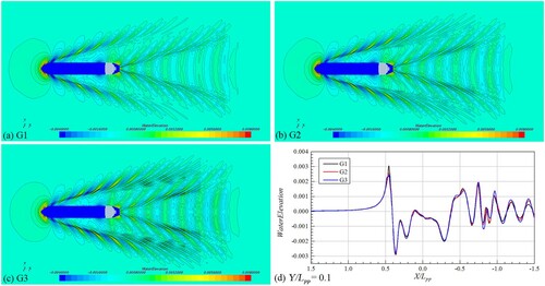
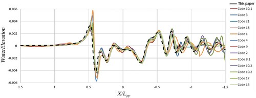
Figure 5 compares the waveform curve at Y/L_PP = 0.1 based on the Grid G1 used in this study to the results from Lloyd's Register (2016). It can be seen that the longitudinal wave cut simulated in this study is very close to the calculation results under the same working conditions (i.e. code2, code9, code10.2, code10.3, code16, code17, and code19) in Lloyd's Register (2016). The waveform peak errors between the calculation results of the above-mentioned working conditions are all within 15%. This also shows the feasibility of the resistance simulation strategy applied in this investigation. The subsequent research on the choice of time step size and wall Y+ value will be based on Grid G1.

Figure 5. Comparison of the longitudinal wave cut at Y/L_PP = 0.1 between this study and Lloyd's workshop.

3.2. Research on setting the time step size

For the standard pseudo-transient resistance calculation, the time step size that is recommended by ITTC (2011) is t = 0.005–0.01 L_PP/v. For more unstable problems, such as those with a low Froude number, a smaller time step size may be needed.

To study the time step sizes that are applicable for the full-scale resistance simulation, four different time step sizes were selected: 0.024, 0.048, 0.096, and 0.192 s corresponding to 0.00125, 0.0025, 0.005, and 0.01 L_PP/v, respectively. In the research on setting the time step size, the Y+ value was also set as 100.

The resistance simulation results for the four different time step sizes are listed in Table 8. In this sea trial, the resistance of REGAL was not measured using LR. Therefore, the average resistance values of the same working conditions (code2, code9, code10.2, code10.3, code16, code17, code19) in LR (2016) were used to verify the simulation results in this study. Table 8 summarises that the overall error of the resistance simulation results for the four time step sizes and result of the LR workshop is within 5%. The ship resistance during the 0.005 and 0.01 L_PP/v time step sizes significantly increased in comparison to the other two small time stepsizes.

Table 8. Resistance simulation results of the REGAL based on the four time step sizes.

Time step size	Resistance (kN)	Error (%)
Average resistance in the LR Workshop (kN) (minimum/max)	292.3
	(285/300.5)
t = 0.024 s (0.00125 LPP/v)	289.7	−0.89
t = 0.048 s (0.0025 LPP/v)	291.4	−0.31
t = 0.096 s (0.005 LPP/v)	303.5	3.83
t = 0.192 s (0.01 LPP/v)	306.5	4.86

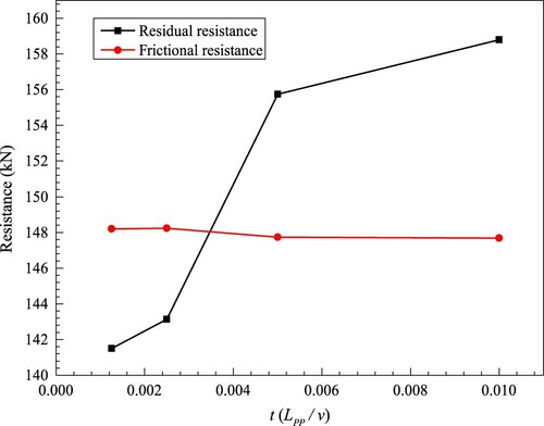
Figure 6 displays the variation of the ship resistance components with the time step size. The figure shows that the ship frictional resistance hardly changes with the time step size, and the residual resistance is greatly affected by the time step size. When t = 0.0025 L_PP/v is increased to 0.005 L_PP/v, the residual resistance suddenly changes, which results in a larger error for the ship resistance under time step sizes of 0.005 and 0.01 L_PP/v.

Figure 6. Ship resistance component of the REGAL at different time step sizes.

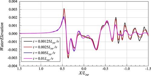
To analyse the reasons for the change in the ship residual resistance, the waveforms for the different time step sizes were analysed; the results are shown in Figures 7 and 8. As can be seen from the figures, the time step size has a greater influence on the evolution and capture of the waveform. When the time steps are 0.00125 L_PP/v and 0.0025 L_PP/v, the overall waveform and the longitudinal wave cut simulation results are relatively close. However, when the time step sizes are 0.005 and 0.01 L_PP/v, the free surface capture problem occurs, and the waveform does not develop correctly and fully, which affects the wave-making resistance.

Figure 7. Free surface waveform of the REGAL at different time step sizes.

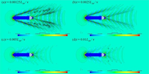
Figure 8. Comparison of the longitudinal wave cut at Y/L_PP = 0.1 between different time step sizes.

The CFL number is an important condition for evaluating numerical calculations, and its distribution on the free surface is shown in Figure 9. It can be seen that the CFL number on the free surface is closely related to the grid size at that location (Figure 3 (a)). The CFL number at the minimum grid is the largest, which is about 0.8 and 1.6 under the time step sizes of 0.0025 L_PP/v and 0.005 L_PP/v, respectively. Owing to the obvious difference of the free surface waveforms under the two working conditions, it is recommended that the CFL number on the free surface in the full-scale ship simulation be within 1.

Figure 9. CFL number on the free surface at different time step sizes.

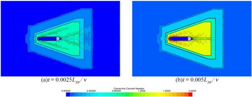
Figure 10 shows the nominal wake field (without the hub) of the REGAL at different time step sizes. The simulation results clearly capture the presence of the hook-shaped velocity contours for this ship type (Guo et al., 2018). However, when the time step size increases, some differences between the velocity profiles of the wake field appear. The axial velocities at different propeller radii on the propeller disk were extracted; the results are given in Figure 11. The definition of the abscissa θ in Figure 11 is given in Figure 10(a).

Figure 10. Nominal wake field of the REGAL at different time step sizes.

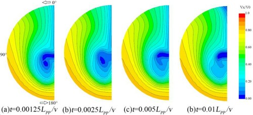
Figure 11. Circumferential distribution of axial velocity at different radii.

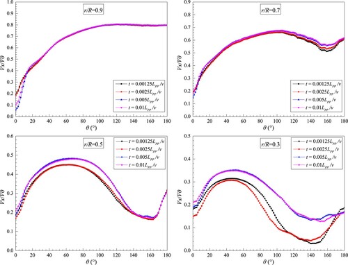
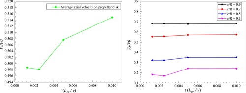
As can be seen from Figure 11, when the time step sizes are 0.00125 and 0.0025 L_PP/v, the velocity profiles are almost the same, but when those are 0.005 L_PP/v or 0.01 L_PP/v, the velocity values at r/R = 0.3 and r/R = 0.5 increase significantly. The average non-dimensional axial velocity on the propeller disk and different radii at different time step sizes is shown in Figure 12. The difference between the average axial velocity on the propeller disk when the time step sizes are 0.0025, 0.005 L_PP/v, or 0.01 L_PP/v and that when the time step size is 0.00125 L_PP/v is 0.11%, 2.87%, or 3.24%, respectively.

Figure 12. Average axial velocity on the propeller disk (left) and different radii (right) at different time step sizes.

Based on the analysis of the ship resistance components, waveforms, and wake fields for the different time step sizes, the time step size for the resistance simulation of the full-scale ships (low speed ship form) should ensure that the CFL number on the free surface is not greater than 1, and the recommended value is 0.0025 L_PP/v.

3.3. Choosing the wall Y+ value

When extrapolating the ship resistance, the prediction of the frictional resistance is generally based on the ITTC1957 line. With the development of the full-scale simulation, many researchers have determined a certain error between the full-scale ship frictional resistance simulation value and the ITTC1957 line. Subsequently, Grigson (1993) and Katsui (2005) proposed new empirical formulas for the frictional resistance, which were recognised to a certain extent (Park et al., 2015).

The ITTC 1957 line, Grigson line, and Katsui line of friction resistance are respectively expressed as follows: (12) $\begin{array}{rl}{C}_f& =\frac{0.075}{{(\lg Re-2)}^2}\end{array}$(12) (13) $\begin{array}{rl}{C}_f& =\{\begin{array}{l}[0.93+0.1377(\log Re-6.3{)}^2\\ -0.06334(\log Re-6.3{)}^4]\times \frac{0.075}{(\log Re-2{)}^2},1.5\\ \times {10}^6\le Re\le 2\times {10}^7\\ [1.032+0.02816(\log Re-8)\\ -0.006273(\log Re-8{)}^2]\times \frac{0.075}{(\log Re-2{)}^2},{10}^8\\ \le Re\le 4\times {10}^9\end{array}\end{array}$(13) (14) $\begin{array}{rl}{C}_f& =\frac{0.0066577}{{(\log Re-4.3762)}^{0.042612\log Re+0.56725}}\end{array}$(14)

Here, Re is the Reynolds number.

The wall Y+ value is an important basis for measuring the ship boundary layer mesh whose quality is related to the simulation accuracy in the boundary layer flow, and it has a greater influence on the accuracy of simulating the viscous resistance of ship.

To analyse the wall Y+ value of the ship surface that is suitable for a full-scale simulation, referring to the range of wall Y+ values selected in the LR Workshop (Table 5), six different target wall Y+ values were selected (with constant prism layer thickness, while adjusting the number (10–14) and stretching (1.05–1.2) the boundary layer mesh): 60, 100, 200, 300, 500, and 800. In the wall Y+ value convergence study, the simulation is based on Grid G1, and the time step size is 0.048 s, which corresponds to 0.0025L_PP/v. The different wall Y+ distributions on the surface of the REGAL are shown in Figure 13. It can be seen that the Y+ value on the hull surface is slightly smaller than the target Y+ value on the whole. The distribution range of the Y+ value on the hull surface below the waterline is given in Table 9.

Figure 13. Different wall Y+ values on the REGAL surface.

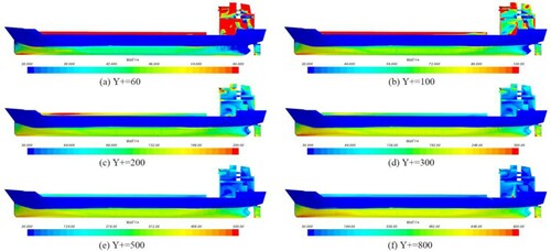
Table 9. Distribution range of Y+ on the hull surface.

Target Y+	60	100	200	300	500	800
Range of Y+	10–100	15–130	25–280	50–410	80–700	100–1000

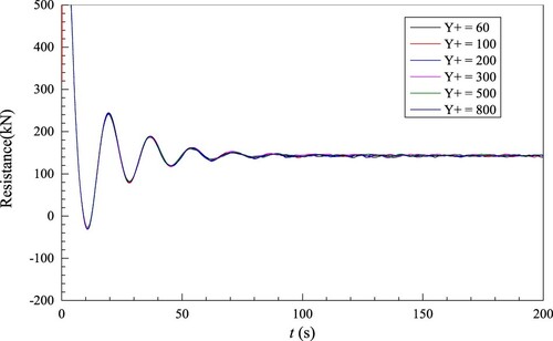
Figure 14 shows the time history of half ship resistance at different Y+ conditions. It can be seen that the resistance tends to converge around 100 s, the simulation physical time of each working condition is 200 s, and the resistance is taken as the average of the interval of 100–200 s.

Figure 14. Time history of half ship resistance at different Y+ values.

The ship resistance components for the different wall Y+ values were monitored, and the changes in the residual resistance and frictional resistance with the wall Y+ value are shown in Figure 15. It can be seen that the residual resistance is almost stable when the wall Y+ value is 60, 100, or 200; a slight increase occurs when the wall Y+ value is greater than 300. When it is below 300, the simulated frictional resistance basically remains unchanged, which is in good agreement with both the Katsui line and the Grigson line. When Y+ is 500–800, the frictional resistance of the ship increases to a certain extent. The difference between the total resistance of the ship when the wall Y+ value is 100, 200, 300, 500, or 800 and the total resistance when the wall Y+ value is 60 is 0.15%, 0.23%, 1.07%, 1.43%, or 1.86%, respectively.

Figure 15. Ship resistance component of the REGAL with different wall Y+ values.

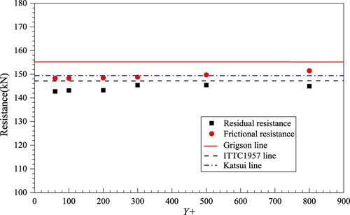
Figure 16 represents the skin friction coefficient on the REGAL for different wall Y+ values. It can be seen that the skin friction coefficient of the bow and stern increases with the wall Y+ value, particularly when Y+ is greater than 200. This is related to the difference in the simulation of the boundary layer flow under the different wall Y+. Figure 17 presents the distribution of the pressure coefficient (Song et al., 2018) on the stern for different wall Y+ values. As can be seen, when Y+ is 300, 500, and 800, the pressure at the stern decreases to a certain extent, which increases the pressure difference between the bow and the stern, consequently increasing the viscous pressure resistance.

Figure 16. Skin friction coefficient on the REGAL at different wall Y+ values.

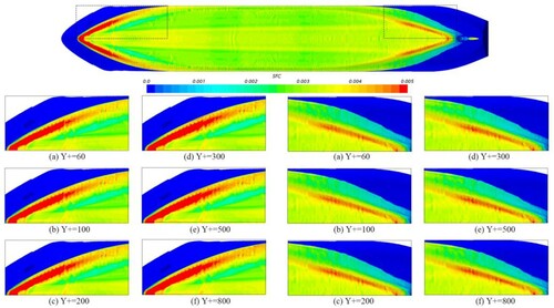
Figure 17. Pressure coefficient on the REGAL at different wall Y+ values.

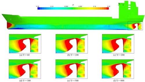
Figures 18 and 19 represent the free surface waveform and the longitudinal wave cut at Y/L_PP = 0.1 under different wall Y+ conditions, respectively. It can be seen that the calculation results of the waveform under different Y+ value conditions are very similar with some differences only at the bow waveforms, which is also related to the evolution in the boundary layer flow. The changes in the skin friction coefficient, pressure difference, and waveform under different working conditions explain the difference in the ship resistance in Figure 15.

Figure 18. Free surface waveform of the REGAL at different wall Y+ values.

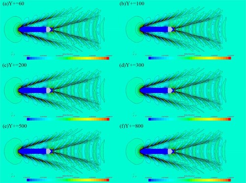
Figure 19. Comparison of the longitudinal wave cut at Y/L_PP = 0.1 between different wall Y+ conditions.

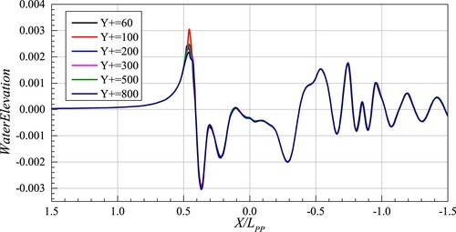
Figure 20 shows the nominal wake field of the REGAL at different wall Y+ values. It can be seen from the figure that when the wall Y+ value is greater than 300, the shape of the vortex structure shows a certain difference. The velocities at different propeller radii on the propeller disk were extracted; the results are given in Figure 21. It can be seen that with the decrease in r/R, the difference in the velocity under different conditions is greater. In other words, the closer to the center of the propeller disk, the greater is the influence of the Y+ value on the velocity. The velocity profile when Y+ is 500 and 800 is obviously different from other working conditions.

Figure 20. Nominal wake field of the REGAL at different wall Y+ values.

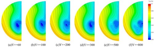
Figure 21. Circumferential distribution of axial velocity at different radii.

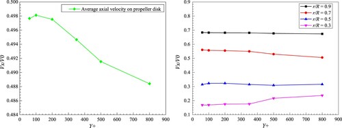
To analyse quantitatively the influence of the wall Y+ value, the average non-dimensional axial velocity of the propeller disk (without installing the false hub) and different radii was obtained; the results are illustrated in Figure 22. Figure 22 shows that when wall Y+ is less than 200, the mean velocity of the propeller disk surface and different radii remains stable. When wall Y+ is greater than 200, the average velocity at r/R = 0.3 increases, the average velocity at r/R = 0.5 and r/R = 0.7 decreases, and that on the propeller disk decreases to a certain extent. The difference between the average axial velocity on the propeller disk when the wall Y+ value is 100, 200, 300, 500, or 800, and the axial velocity when the wall Y+ value is 60 is 0.08%, –0.03%, 0.61%, 1.23%, or 1.84%, respectively.

Figure 22. Average axial velocity on the propeller disk (left) and different radii (right) at different wall Y+ values.

Based on the simulation results of the resistance, propeller disk velocity, and flow field in this section, it is considered appropriate that the Y+ value when performing full-scale ship simulation is within 200.

4. Self-propulsion simulations

The self-propulsion strategy was studied based on the resistance simulation strategy. The hull Y+ value and the grid topology remained the same as in the resistance simulation. The grid number for the self-propulsion simulation was 30.22 million. The specific grid settings are listed in Section 2.5. According to the sea trial results given by Lloyd's Register (2016), when the propeller revolution speed is 106.4 RPM, the ship speed is 13.05 knots (the corresponding Froude number is 0.182). The main purpose of this part is to determine a suitable time step size for the ship self-propulsion calculation; hence, the simulated speed is 13.05 knots, and the propeller revolution speed is constantly 106.4 RPM.

In Lloyd's Register (2016), the time step size of the self-propulsion is mostly 1–5°/step, but some organisations set it to 10°, 20°, or even 89°/step. In this study, the five selected time step sizes were 0.000783 s (0.000038 L_PP/v), 0.001566 s (0.000076 L_PP/v), 0.003133 s (0.000152 L_PP/v), 0.006266 s (0.000305 L_PP/v), and 0.01253 s (0.00061 L_PP/v), and the corresponding equivalent angle of rotation for the time step size is 0.5°/step, 1°/step, 2°/step, 4°/ step, and 8°/step, respectively. Figures 23–25 in this section display all the simulated results for 1°/step.

Figure 23. Simulated propeller thrust and torque for the different time step sizes

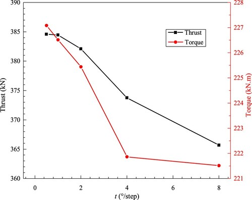
Figure 24. Simulated thrust deduction fraction at the different time step sizes.

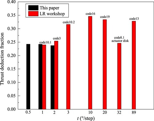
Figure 25. CFL number on the interface of sliding mesh at different time step sizes.

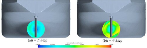
Table 10 and Figure 23 compare the computed and trial results of the thrust and torque. As evident from Table 11, the thrust and torque are relatively less sensitive to the time step size. The error of the thrust and torque was less than 4% for all five time step sizes. By conducting an analysis, the thrust and torque decrease with an increase in the time step size. The changes in the thrust and torque are relatively small at 0.5–2°/step, but a sudden drop occurs at 4°/step. It should be noted that the resistance at different propeller revolution speeds is 370–375 kN, and the difference between the resistance and thrust at different time step sizes is in the range −2.48–3.94%. The two limits are relatively close, which suggests that the ship is in a self-propelled state.

Table 10. Computed and trial results of the propeller thrust and torque.

Time step size	CPU time (h)	Thrust (kN)	Error (%)	Torque (kN.m)	Error (%)
Trial data obtained by the LR		376.91		229.7
0.5°/step	32×200	384.58	2.03	227.08	−1.14
1°/step	32×150	384.46	2.00	226.51	−1.39
2°/step	32×130	382.10	1.38	225.44	−1.85
4°/step	32×104	373.76	−0.84	221.86	−3.42
8°/step	32×90	365.69	−2.98	221.51	−3.57

Table 11. Time step sizes of the self-propulsion simulations.

Item	Absolute time (s)	Angular equivalent	Time step size
1	0.000783	0.5°/step	0.000038 LPP/v
2	0.001566	1°/step	0.000076 LPP/v
3	0.003133	2°/step	0.000152 LPP/v
4	0.006266	4°/step	0.000305 LPP/v
5	0.01253	8°/step	0.00061 LPP/v

The simulation results of the thrust deduction fraction in this study to the results of Lloyd's Register (2016) for the different time step sizes are compared in Figure 24. It is seen that the results from this study are consistent with the results from Lloyd's Register (2016) for the same time step size. The virtual disk model was used by Code8.1 to simulate the self-propulsion, and it obtained an acceptable thrust deduction fraction for a relatively long time step size; this is the advantage of the virtual disk model. By simulating the self-propulsion based on the propeller rotation, the thrust deduction fraction is more reliable when the time step size is less than 2°/ step (0.000152 L_PP/v).

Figure 25 shows the CFL number distribution on the interface of the sliding mesh. As can be seen, the CFL numbers at 2°/step and 4°/step are approximately 0.7 and 1.4, respectively. As there is considerable difference between the thrust and torque under the two time step sizes, it should be ensured that the CFL number on the interface of the slip mesh be not more than 1.

Figures 26 and 27 show the distribution of the pressure coefficients and skin friction coefficient on the REGAL under different conditions, respectively. As can be seen, the difference in the two distributions between the resistance and self-propulsion conditions is mainly at the stern. This is because the running of the propeller causes an increase in the water velocity in front of it, which decreases the pressure coefficient and increases the friction coefficient of the stern.

Figure 26. Pressure distribution on the REGAL for the resistance (a) and self-propulsion (b) conditions.

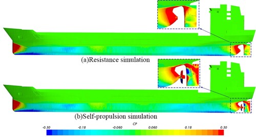
Figure 27. Skin friction coefficient on the REGAL for the resistance (a) and self-propulsion (b) conditions.

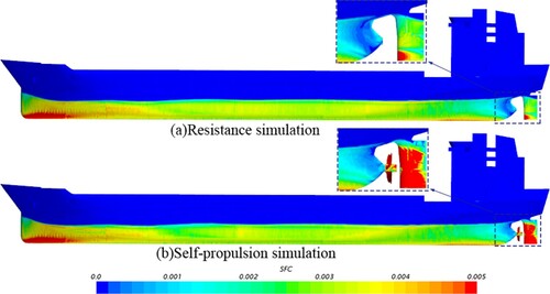
Figure 28 shows the velocity distribution at the cross-section X/D = 0.2315 that is downstream of the propeller disk for the resistance and self-propulsion condition. In the resistance simulation, the hook-shaped velocity profile for this type of ship was clearly captured. The velocity contour plot of the self-propulsion simulation demonstrates clearly the wake asymmetry. In addition, the low-speed region caused by the hub vortex is also well displayed in this section.

Figure 28. Velocity contour plots of the cross-section X/D = 0.2315 that is downstream of the propeller disk for the resistance (left) and self-propulsion (right) condition.

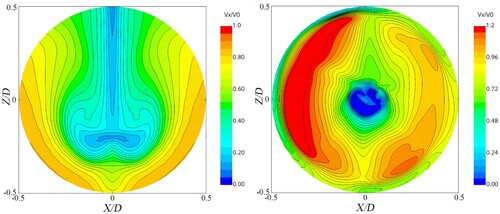
Figure 29 depicts the propeller vortex structure, where the iso-surface was rendered by $Q=0.5(||\Omega |{|}^2-||S|{|}^2)=50$, in which S and Ω denote the strain rate and vorticity rate magnitude, respectively. The unsteady characteristics of the propeller wake can be clearly observed from the figure. Therefore, in self-propulsion simulations, many researchers have focused on the unsteady characteristics of the propeller in addition to the self-propulsion factors. The propeller excitation force is the main source for the structural vibration of the stern and that induced by the excitation force that causes damage to the hull structure (Paik et al., 2010). The unsteady thrust and torque for the different time step sizes were calculated based on the fast Fourier transform; the results are displayed in Figure 30.

Figure 29. Vortical structures around propeller and rudder

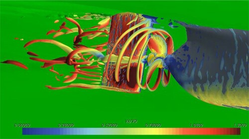
Figure 30. Frequency domain results of thrust (a) and torque (b) for different time step sizes.

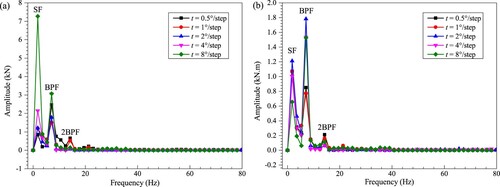
Figure 30 shows that the propeller behind the REGAL ship has a fluctuating amplitude at the shaft frequency (SF, 1.773 Hz) and the blade passage frequency (BPF, 7.093 Hz). However, there is a certain gap in the frequency domain results for each time step size. The SF excitation force is mainly caused by the mechanical imbalance, which is due to the installation process of the propeller or the stern asymmetry.

In Lloyd's Register (2016), owing to the large time step size used by some organisations or the use of the virtual disk model, only three organisations provided the frequency domain results of the thrust and torque at 13.05 knots.

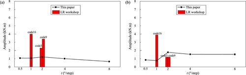
The fluctuation amplitudes at the SF and BPF simulated in this study and that of Lloyd's Register (2016) are compared in Figures 31 and 32, respectively. It is seen that the simulation results in this study and the workshop results have a certain degree of agreement under some working conditions. The amplitudes of the code3, code9, and code16 in Lloyd's Register (2016) did not seem to be dependent on the time step size, which may be due to the difference between the numerical simulation strategies. For the simulation results in this study, the amplitude of the excitation force shows the influence of the time step size, especially when the 8°/step calculation results differ. The SF amplitude of the thrust and the BPF amplitude of the torque increase with the time step size. Meanwhile, the BPF amplitude of the thrust and SF amplitude decrease with an increase in the time step size. In addition, the fluctuation amplitudes of the thrust and torque at 0.5°/step and 1°/step have a high similarity. Therefore, it is recommended that the time step size should not be greater than 1°/step (0.000076 L_PP/v) when solving the propeller-induced excitation force.

Figure 31. SF amplitude of thrust (a) and torque (b) at different time step sizes.

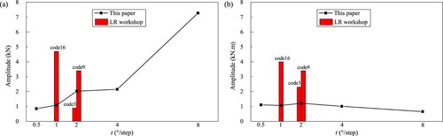
Figure 32. BPF amplitude of thrust (a) and torque (b) at different time step sizes.

5. Conclusions and future work

Using the general cargo vessel REGAL, we investigated the full-scale ship resistance and self-propulsion simulation for various wall Y+ values, time step sizes, and grid numbers. Based on the analysis of the resistance component, waveform, hull pressure, CFL number, wake field, and excitation force, a strategy for simulating the full-scale ship powering performance was obtained. This simulation strategy will have a certain guiding significance for subsequent researchers to perform full-scale simulation research. The following conclusions can be drawn from this study.

1. Both Katsui and Grigson lines are in good agreement with the simulated frictional resistance, which can be used to verify the frictional resistance simulation value.

2. The wall Y+ value will affect the capture of boundary layer flow, evolution of the ship pressure field, and waveform, which can subsequently affect the ship resistance. Based on the simulation results of REGAL, it is considered appropriate if the Y+ value when simulating the powering performance of full-scale ship simulation is within 200.

3. The waveform evolution of the full-scale ship resistance simulation is greatly influenced by the time step size. The time step size for the resistance simulation should meet the requirement that the CFL number on the free surface is not greater than 1; the recommended value is 0.0025 L_PP/v.

4. When the grid topology and time step size are reasonable, the influence of the grids number is not obvious. The full-scale ship resistance can be accurately simulated with tens of millions or millions of grids.

5. When simulating the self-propulsion of a full-scale ship based on the sliding mesh, the CFL number on the interface should not be greater than 1, which is a condition that must be considered. To obtain the correct value for the propeller excitation force, it is recommended that the time step size not be greater than 1°/step (0.000076 L_PP/v).

Presently, there are few open test datasets for full-scale ship sea trials. The REGAL’s published trial data from Lloyd's Register (2016) can provide verification data for the powering performance simulation of full-scale ships. In addition, it can increase researchers’ confidence in the CFD of full-scale ship. Owing to the lack of sea trial data, we used only the REGAL ship for conducting systematic resistance and self-propulsion research, and therefore, the conclusion of this study may be too generalised. In future, full-scale ship simulations of more ship types (e.g. tankers and surface ships) will be carried out, which will support and verify this simulation strategy. In addition, the sea trials by LR did not measure ship resistance, but only obtained self-propulsion data. While researching resistance simulation strategies, we obtained the trend of ship resistance, wake, and other data with time step size and Y+ value through variable parametric analysis and then proposed corresponding guidance and suggestions. However, owing to the lack of the corresponding resistance and wake test results by sea trials, the conclusion is slightly insufficient. The more systematic and comprehensive sea trials in the future can provide more powerful data support for the numerical study of full-scale ship poweringperformance.

Acknowledgments

This work was supported by the Ph.D. Student Research and Innovation Fund of the Fundamental Research Funds for the Central Universities (3072020GIP0104), the National Natural Science Foundation of China (51679052), and the Key Laboratory Fund for Equipment Pre-research (61422230203182223010).

Disclosure statement

No potential conflict of interest was reported by the author(s).

Additional information

Funding

This work was supported by National Natural Science Foundation of China: [Grant Number 51679052]; Key Laboratory Fund for Equipment Pre-research: [Grant Number 61422230203182223010]; the Ph.D. Student Research and Innovation Fund of the Fundamental Research Funds for the Central Universities: [Grant Number 3072020GIP0104].

References

- Bhushan, S., Xing, T., Carrica, P., & Stern, F. (2007). Model-and full-scale URANS/DES simulations for Athena r/v resistance, powering, and motions [paper presentation]. 9th International Conference on Numerical Ship Hydrodynamics, Ann Arbor, MI, USA.
- Bhushan, S., Xing, T., Carrica, P., & Stern, F. (2009). Model- and full-scale URANS simulations of Athena resistance, powering, seakeeping, and 5415 Maneuvering. Journal of Ship Research, 53(4), 179–198. https://doi.org/https://doi.org/10.5957/jsr.2009.53.4.179
- Castro, A. M., Carrica, P. M., & Stern, F. (2011). Full scale self-propulsion computations using discretized propeller for the KRISO container ship KCS. Computers & Fluids, 51(1), 35–47. https://doi.org/https://doi.org/10.1016/j.compfluid.2011.07.005
- Dogrul, A., Song, S., & Demirel, Y. K. (2020). Scale effect on ship resistance components and form factor. Ocean Engineering, 209, 107428. https://doi.org/https://doi.org/10.1016/j.oceaneng.2020.107428
- Farkas, A., Degiuli, N., & Martić, I. (2018). Assessment of hydrodynamic characteristics of a full-scale ship at different draughts. Ocean Engineering, 156, 135–152. https://doi.org/https://doi.org/10.1016/j.oceaneng.2018.03.002
- Grigson, C. W. (1993). An accurate smooth friction line for use in performance prediction. Transactions of the Royal Institution of Naval Architects Part A, 135, 149–162.
- Guo, C. Y., Wu, T. C., Luo, W. Z., Chang, X., Gong, J., & She, W. X. (2018). Experimental study on the wake fields of a Panamax Bulker based on stereo particle image velocimetry. Ocean Engineering, 165, 91–106. https://doi.org/https://doi.org/10.1016/j.oceaneng.2018.07.037
- Hasselaar, T. W. F., & Xing-Kaeding, Y. (2017). Evaluation of an energy saving device via validation speed/power trials and full scale CFD investigation. International Shipbuilding Progress, 63(3–4), 1–27. https://doi.org/https://doi.org/10.3233/ISP-170127
- Hochkirch, K., & Mallol, B. (2013). On the importance of full-scale CFD simulations for ships. 1st International Conference on Computer and IT Applications in the Maritime Industries, COMPIT.
- ITTC. (2011). Practical Guidelines for Ship CFD Applications, No. 7.5-03-02-03.
- Jasak, H., Vukčević, V., Gatin, I., & Lalovic, I. (2019). CFD validation and grid sensitivity studies of full-scale ship self-propulsion. International Journal of Naval Architecture and Ocean Engineering, 11(1), 33–43. https://doi.org/https://doi.org/10.1016/j.ijnaoe.2017.12.004
- Katsui, T. (2005). The proposal of a new friction line. In 5th Osaka colloquium on advanced CFD applications to ship flow and hull form design, Osaka, Japan.
- Kawamura, T., Ouchi, K., & Nojiri, T. (2012). Model and full scale CFD analysis of propeller boss cap fins (PBCF). Journal of Marine Science and Technology, 17(4), 469–480. https://doi.org/https://doi.org/10.1007/s00773-012-0181-2
- Kim, Y. C., Kim, K. S., Kim, J., Kim, Y., Park, I. R., & Jang, Y. H. (2017). Analysis of added resistance and seakeeping responses in head sea conditions for low-speed full ships using URANS approach. International Journal of Naval Architecture and Ocean Engineering, 9(6), 641–654. https://doi.org/https://doi.org/10.1016/j.ijnaoe.2017.03.001
- Kok, Z., Duffy, J., Chai, S., Jin, Y., & Javanmardi, M. (2020). Numerical investigation of scale effect in self-propelled container ship squat. Applied Ocean Research, 99, 102143. https://doi.org/https://doi.org/10.1016/j.apor.2020.102143
- Koushan, K., Krasilnikov, V., Nataletti, M., Sileo, L., & Spence, S. (2020). Experimental and numerical study of pre-swirl stators PSS. Journal of Marine Science and Engineering, 8(1), 47. https://doi.org/https://doi.org/10.3390/jmse8010047
- Lloyd's Register. (2016). A Workshop on Ship Scale Hydrodynamic Computer Simulation. https://www.lr.org/en/insights/articles/findings-of-lrs-full-scale-numerical-modelling-workshop/.
- Lu, Y., Chang, X., Chuang, Z., Xing, J., Zhou, Z., & Zhang, X. (2020). Numerical investigation of the unsteady coupling airflow impact of a full-scale warship with a helicopter during shipboard landing. Engineering Applications of Computational Fluid Mechanics, 14(1), 954–979. https://doi.org/https://doi.org/10.1080/19942060.2020.1786461
- Niklas, K., & Pruszko, H. (2019). Full scale CFD seakeeping simulations for case study ship redesigned from V-shaped bulbous bow to X-bow hull form. Applied Ocean Research, 89, 188–201. https://doi.org/https://doi.org/10.1016/j.apor.2019.05.011
- Paik, B. G., Kim, K. Y., Kim, K. S., Park, S., Heo, J., & Yu, B. S. (2010). Influence of propeller wake sheet on rudder gap flow and gap cavitation. Ocean Engineering, 37(16), 1418–1427. https://doi.org/https://doi.org/10.1016/j.oceaneng.2010.07.002
- Park, S., Oh, G., Rhee, S. H., Koo, B. Y., & Lee, H. (2015). Full scale wake prediction of an energy saving device by using computational fluid dynamics. Ocean Engineering, 101, 254–263. https://doi.org/https://doi.org/10.1016/j.oceaneng.2015.04.005
- Ponkratov, D., & Zegos, C. (2015). Validation of ship scale CFD self-propulsion simulation by the direct comparison with sea trials results [paper presentation]. 4th International Symposium on Marine Propulsors SMP’15, Austin, Texas, USA.
- Ponkratov, D. D. (2015). DES prediction of cavitation erosion and Its validation for a Ship Scale propeller. Journal of Physics: Conference Series, 656, 012055. https://doi.org/https://doi.org/10.1088/1742-6596/656/1/012055
- Raven, H. C., Van der Ploeg, A., & Starke, A. R. (2008). Towards a CFD-based prediction of ship performance—progress in predicting full-scale resistance and scale effects. International Journal of Maritime Engineering, 150, 31–42.
- Salih, S. Q., Suliman, M., Rasani, M. R., Ariffin, A. K., Mohammad, T., Shah, Y., Ya, T., Al-Ansari, N., Mundher, Z., Chau, K. W., & Yaseen, Z. M. (2019). Thin and sharp edges bodies-fluid interaction simulation using cut-cell immersed boundary method. Engineering Applications of Computational Fluid Mechanics, 13(1), 860–877. https://doi.org/https://doi.org/10.1080/19942060.2019.1652209
- Saydam, A. Z., Gokcay, S., & Insel, M. (2018). CFD based vortex generator design and full-scale testing for wakenon-uniformity reduction. Ocean Engineering, 153, 282–296. https://doi.org/https://doi.org/10.1016/j.oceaneng.2018.01.097
- Song, K., Guo, C., Gong, J., Li, P., & Wang L. (2018). Influence of interceptors, stern flaps, and their combinations on the hydrodynamic performance of a deep-vee ship. Ocean Engineering, 170, 306–320. https://doi.org/https://doi.org/10.1016/j.oceaneng.2018.10.048
- Song, K., Guo, C., Wang, C., Sun, C., Li, P., & Zhong, R. (2020). Experimental and numerical study on the scale effect of stern flap on ship resistance and flow field. Ships and Offshore Structures, 15(9), 981–997. https://doi.org/https://doi.org/10.1080/17445302.2019.1697091
- Song, S., Demirel, Y. K., & Atlar, M. (2019). An investigation into the effect of biofouling on the ship hydrodynamic characteristics using CFD. Ocean Engineering, 175, 122–137. https://doi.org/https://doi.org/10.1016/j.oceaneng.2019.01.056
- Stern, F., Wilson, R. V., Coleman, H. W., & Paterson, E. G. (2001). Comprehensive approach to verification and validation of CFD simulations—part 1: Methodology and procedures. Journal of Fluids Engineering, 123(4), 793–802. https://doi.org/https://doi.org/10.1115/1.1412235
- Su, D., Xu, G., Huang, S., & Shi, Y. (2019). Numerical investigation of rotor loads of a shipborne coaxial-rotor helicopter during a vertical landing based on moving overset mesh method. Engineering Applications of Computational Fluid Mechanics, 13(1), 309–326. https://doi.org/https://doi.org/10.1080/19942060.2019.1585390
- Sun, S., Chang, X., Guo, C., Zhang, H., & Wang, C. (2019). Numerical investigation of scale effect of nominal wake of four-screw ship. Ocean Engineering, 183, 208–223. https://doi.org/https://doi.org/10.1016/j.oceaneng.2019.04.032
- Sun, W., Hu, Q., Hu, S., Su, J., Xu, J., Wei, J., & Huang, G. (2020). Numerical analysis of full-scale ship self-propulsion performance with direct comparison to statistical sea trail results. Journal of Marine Science and Engineering, 8(1), 24. https://doi.org/https://doi.org/10.3390/jmse8010024
- Tahara, Y. (2002). Computation of ship viscous flow at full scale Reynolds number. The Japan Society of Naval Architects and Ocean Engineers, 2002(192), 89–101. https://doi.org/https://doi.org/10.2534/jjasnaoe1968.2002.89
- Tezdogan, T., Demirel, Y. K., Kellett, P., Khorasanchi, M., Incecik, A., & Turan, O. (2015). Full-scale unsteady RANS CFD simulations of ship behaviour and performance in head seas due to slow steaming. Ocean Engineering, 97, 186–206. https://doi.org/https://doi.org/10.1016/j.oceaneng.2015.01.011
- Tezdogan, T., Incecik, A., & Turan, O. (2016). Full-scale unsteady RANS simulations of vertical ship motions in shallow water. Ocean Engineering, 123, 131–145. https://doi.org/https://doi.org/10.1016/j.oceaneng.2016.06.047
- Visonneau, M. (2005). A step towards the numerical simulation of viscous flows around ships at full scale - Recent achievements within the European Union Project EFFORT. Royal Institute of Naval Architecture Marine CFD, Southampton, France.
- Visonneau, M., Queutey, P., & Deng, G. B. (2006). Model and full-scale free surface viscous flows around fully-appended ships. ECCOMAS CFD 2006, Egmond aan Zee, Holland.
- Wang, L., Guo, C., Su, Y., Xu, P., & Wu, T. (2017). Numerical analysis of a propeller during heave motion in cavitating flow. Applied Ocean Research, 66, 131–145. https://doi.org/https://doi.org/10.1016/j.apor.2017.05.001
- Wang, L., Guo, C., Xu, P., & Su, Y. (2019). Analysis of the wake dynamics of a propeller operating before a rudder. Ocean Engineering, 188, 106250. https://doi.org/https://doi.org/10.1016/j.oceaneng.2019.106250
- Wang, L., Martin, J. E., Felli, M., & Carrica, M. C. (2020). Experiments and CFD for the propeller wake of a generic submarine operating near the surface. Ocean Engineering, 206, 107304. https://doi.org/https://doi.org/10.1016/j.oceaneng.2020.107304
- Wang, L. Z., Guo, C. Y., Su, Y. M., & Wu, T. (2018). A numerical study on the correlation between the evolution of propeller trailing vortex wake and skew of propellers. International Journal of Naval Architecture and Ocean Engineering, 10(2), 212–224. https://doi.org/https://doi.org/10.1016/j.ijnaoe.2017.07.001
- Wang, Z., Xiong, Y., Wang, R., Shen, X., & Zhong, C. (2015). Numerical study on scale effect of nominal wake of single screw ship. Ocean Engineering, 104(1), 437–451. https://doi.org/https://doi.org/10.1016/j.oceaneng.2015.05.029
- Xing, T., & Stern, F. (2010). Factors of safety for Richardson extrapolation. Journal of Fluids Engineering, 132(6), 061403. https://doi.org/https://doi.org/10.1115/1.4001771
- Zhang, H., Zhang, H., Chen, X., Liu, H., & Wang, X. (2018). Scale effect studies on hydrodynamic performance for DTMB 5415 using CFD [paper presentation]. ASME 2018 37th International Conference on Ocean, Offshore and Arctic Engineering, Madrid, Spain.