Numerical analysis of a new cross-flow type hydraulic turbine for high head and low flow rate

ABSTRACT

Cross-flow turbines have recently been proposed for energy recovery in aqueducts when the outlet pressure is greater than zero, owing to their constructive simplicity and good efficiency within a large range of flow rates and head drops. In the case of high head drop (higher than 150 m) and relatively small discharge (lower than 0.2 m³/s), the traditional design of these turbines leads to very small widths of the nozzle and the runner; as a consequence, friction losses grow dramatically and efficiency drops down to very low values. Standard Pelton turbines require zero outlet pressure and cannot be used as alternatives. A new counter-pressure hydraulic turbine for high head and low flow rate, called the High Power Recovery System (H-PRS) is proposed. H-PRS presents a different geometry to reduce friction losses inside the nozzle and the runner by widening the two external walls. Several curved baffles are proposed to guide the fluid particles inside the nozzle and to guarantee the right velocity direction at the inlet surface of the runner. Computational Fluid Dynamics (CFD) 3D transient analyses are carried out to measure H-PRS efficiency for different operating conditions and to compute its characteristic curve for different positions of the regulating flap.

KEYWORDS:

• Micro-hydropower
• energy recovery
• cross-flow turbine
• water distribution network
• Banki–Michell turbine

1. Introduction

The plan for energy transition in Europe seeks to achieve low-CO₂ electricity production, with a reduced impact on the environment and mitigation of climate change: this is an ambitious plan that is meant to be an example for the entire planet. Hydropower traditionally covers the largest part of renewable energy production in the world, with a large range of nominal power, going from the 18 GW of the three-gorges plant in the Yangtze river, People’s Republic of China, to the few kilowatts produced by off-grid installations. Combining the large economic productivity of hydropower plants with a low environmental impact is one of the major technological challenges of the present day.

To this end, a contribution is made by traditional cross-flow turbines (Adhikari & Wood, 2018; Rantererung et al., 2019; Sammartano et al., 2015, 2016, 2017a; Sinagra et al., 2016; Subekti et al., 2018). These turbines are usually preferred because of their low cost, consistent with the available hydraulic power, usually lower than one megawatt. When the outlet gauge pressure of the turbine is greater than zero, cross-flow turbines cannot be used because they are designed according to the hypothesis of free outlet discharge.

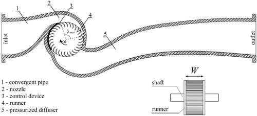
A major contribution to hydropower production is also made by inline turbines installed along transport or even distribution aqueducts designed for domestic consumption (Carravetta et al., 2013, 2014; Delgado et al., 2019; Fecarotta et al., 2015; Giudicianni et al., 2020; Nakamura et al., 2015; Samora et al., 2016; Sammartano et al., 2017b; Simão & Ramos, 2019; Sinagra et al., 2017, 2019, 2020; Vagnoni et al., 2018) or irrigation (Algieri et al., 2020). In contrast to traditional turbines, installed downstream of water reservoir dams and releasing the turbined water inside the river cross section, inline turbines do not require a constant discharge and do not modify the natural hydrological regime inside the river. Inline turbines can replace needle or butterfly valves for discharge regulation, as well as Pressure Reducing Valves (PRVs) already existing along the pipes. These valves play a major role for environment conservation, because pressure reduction is the most efficient way to control water leakage from pipes (Araujo et al., 2006; Gupta et al., 2020; Nourhanm et al., 2017), which usually amounts to 30–40% of the distributed water volume in water distribution networks. In this case, Pump As Turbine (PAT) (Carravetta et al., 2013; Delgado et al., 2019; Giudicianni et al., 2020) or Power Recovery System (PRS) turbines (Sammartano et al., 2017b; Sinagra et al., 2017, 2019, 2020) can provide the same functions as those required by regulation valves. The PRS turbine is a special variant of the cross-flow turbine with pressurized outflow (see a section orthogonal to the turbine axis in Figure 1).

Figure 1. Sections of the traditional PRS turbine.

Further restrictions apply in the case of high head drop (higher than 150 m) and relatively small discharges (lower than 0.2 m³/s). In this range, axial and PRS turbines have low efficiency and only PATs can be applied. On the other hand, hydraulic regulation is missing in PATs and this implies the need to by-pass part of the discharge or to dissipate part of the available head drop when the actual head–discharge point is different from the design one.

Some authors (Kramer et al., 2017) have proposed a special variant of the traditional Pelton turbine (Leman et al., 2019), wherein the water flux goes from the turbine case into a small air-pressurized tank, but at the present time this solution still has several limitations, such as plant efficiency reduction due to the energy needed for the air pressurization, the release of dissolved air downstream of the pipeline and the corresponding augmented corrosion.

The reason of the low efficiency achieved by fully pressurized turbines like PAT or PRS when the design input parameters are high head drop and small discharge is likely to be the high velocity achieved by the water particles within small channel sections inside the nozzle and the runner with resulting energy dissipation due to friction losses. In this study, we test a new geometry for the PRS turbine, called the High Power Recovery System (H-PRS), where a 3D shape of both the nozzle and the runner is adopted in order to limit most of the friction losses to the channels between the curved blades where energy transfer occurs. To test the new geometry, the characteristic curves of a study case, each one for a different position of the regulation flap, are obtained along with the corresponding efficiencies, by means of 14 transient simulations. To test the efficiency of the proposed changes, three other simulations have also been run with fully open flaps. In the first one, the PRS turbine, designed with the same input parameters, has been solved and its efficiency compared with the efficiency of the proposed H-PRS turbine. In the second one, the H-PRS has been solved without baffles inside the nozzle; in the third one, the PRS turbine has been solved assuming a coating of the interior walls made of hydrophobic materials and free-slip boundary conditions. The use of hydrophobic coatings (Dong et al., 2013) could provide a strong increment in turbine efficiency, but the abrasion due to the high velocities occurring in the runner could also have long-term disrupting effects. This last simulation aims to show that friction losses are responsible for the low efficiency attained with 2D geometries.

In Section 2, the design criteria of the PRS turbine are briefly summarized. In the same section, it is also shown that the previous criteria lead to a very small width/diameter (W/D) ratio of the runner in the case of high head drop and small flow rate. A low W/D ratio implies a strong dissipative effect of the lateral impervious surface of the runner disks, resulting in significant efficiency reduction. In Sections 3 and 4, the main geometric changes adopted in the runner and in the stator for the new H-PRS turbine are proposed and motivated. In Section 5, the numerical model used to carry out all the 3D simulations for the next machine characterization is shown. In Section 6, the simulations carried out for machine characterization are described and the efficiency of the designed H-PRS is compared in the case of a fully open flap with (1) the efficiency of the same machine designed without baffles inside the nozzle and (2) the efficiency of a PRS designed by the traditional method (Sinagra et al., 2021) for the same design input data. The second test case is also solved assuming a coating of the interior walls made of hydrophobic material and free-slip boundary conditions. Conclusions follow.

2. External diameter and width design

The external width of the runner and its diameter in the proposed H-PRS are the same as those proposed for the PRS by some of the authors in Sammartano et al. (2017b) and Sinagra et al. (2017, 2020, 2021). PRS is a cross-flow turbine, with a pressurized outlet and a mobile flap aimed at changing the characteristic curve, saving the good efficiency of the device for working points ΔH–Q different from the design one.

In PRS, the diameter D and width W are computed, along with the inlet velocity V, by solving three equations derived from (1) the specific energy balance between the pipe and the inlet surface of the runner, (2) the optimal runner rotational velocity condition and (3) the mass conservation equation. The energy balance leads to the following equation (Sammartano et al., 2016) linking the velocity norm at the inlet surface of the runner with the head drop and the rotational velocity: (1) $V=C_V\sqrt{2g\left(\mathrm{\Delta }H-\xi \frac{{\omega }^2{D}^2}{8g}\right)},$(1) where C_v= 0.98 and ξ = 2.1 are constant coefficients (Sinagra et al., 2017), ΔH is the head drop between the inlet and outlet sections of the PRS, ω is the runner rotational velocity, D is the outer runner diameter and g is the acceleration due to gravity. The optimal rotation velocity is given by (2) $V_r=\frac{2\cdot V\cos \alpha }{\omega D},$(2) where α is the velocity inlet angle with respect to the tangent direction, assumed equal to 15°, and V_r is the optimal value of the ratio between the inlet velocity V and the runner velocity at the inlet surface. This optimal value has been found to be equal to about 1.7 by Sinagra et al. (2020). Equations (1) and (2) can be solved in the V and D unknowns for a given value of the runner rotational velocity ω. In small hydropower plants, the electrical generator is usually of the asynchronous type. For this reason, the rotational velocity ω is a function only of the frequency f of the AC grid (50 Hz in Europe) and of the number p of the polar couples of the selected electrical generator, according to the following equation: (3) $\omega =\frac{2\pi f}{p}$(3)

Finally, the mass conservation equation provides the following width W of the runner: (4) $W=\frac{2Q}{D{\lambda }_{max}V\sin \alpha }$(4) where Q is the flow rate and λ_max is the maximum inlet angle, equal to 90°, as shown in Figure 1.

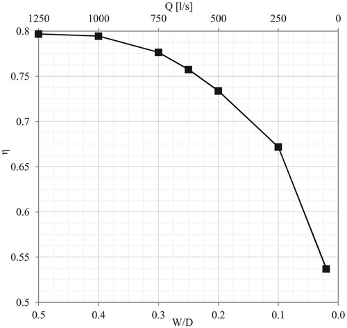
A simple functional analysis of Equations (1)–(4) shows that a reduction of the discharge Q for a fixed ΔH value leads to a reduction of the W/D ratio. This reduction has a negligible impact on the device efficiency up to a sill value of about 0.5. Below this value, the internal surface of the runner disks, because its rotational velocity is lower than that of the particles, provides a consistent friction force with a corresponding energy dissipation and efficiency reduction. See in Figure 2 the efficiencies computed by solving the traditional PRS turbine with the model proposed by Sinagra et al. (2021), assuming ΔH = 200 m, D = 500 mm and a discharge Q = 5 W, where [Q] = l/s and [W] = mm. The efficiencies are defined as (5) $\eta =\frac{P}{\gamma Q\Delta H}$(5) where P is the mechanical power produced and γ is the water specific weight (9807 N/m³).

Figure 2. Efficiency versus W/D ratio and discharge in traditional PRS turbines.

3. H-PRS runner design

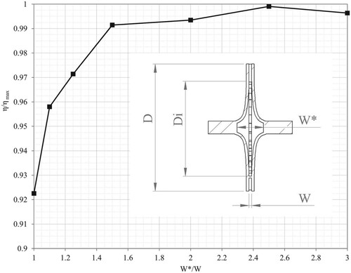
The general strategy proposed here to fill the described technological gap is to reduce the friction losses inside the nozzle and the runner of the H-PRS by widening the two external walls far from the inlet surface of the runner (see the axial section in Figure 3). For the runner itself, this goal is achieved by saving the planar shape of the external disks only inside the two annuli holding the turbine blades. For smaller distances from the runner axis, below the inner radius R_i of the annulus, we move from a planar shape to a curved one. For distances r < R_i, the norm of the velocity relative to the rotating system is assumed to remain constant along with the radius, in contrast to the original PRS, where the norm of the particle velocities grows after crossing the first blade channel up to the minimum distance from the axis and then drops again up to the inlet of a new blade channel. Assuming that, at least for a small distance from the inlet surface, the relative velocities maintain a radial direction, a constant velocity norm is equivalent to a constant area S_c crossed by the water flow at a given distance r from the axis of the runner, due to mass conservation.

Figure 3. Runner efficiency versus W*/W ratio.

This can be written as (6) $S_c\left(r\right)=W\left(r\right)r{\lambda }_{max}=W{R}_i{\lambda }_{max}$(6) where the diameter D_i = 2R_i is set equal to 0.75 D (Sammartano et al., 2017b) and W(r) is the wall distance in the axial direction. Since W(r) is a hyperbolic function, we need to fix a limit W = W* for small r values.

See the axial section of the H-PRS runner in Figure 3 designed in the next study case of Section 6 according to Equation (6). In Figure 3, the relative efficiencies of seven different runners, adopted for the same turbine solved with the numerical model described in the Section 5, are plotted versus the W*/W ratio. The efficiencies, scaled with respect to the maximum 71.7% value, remain almost constant for W*/W ratios greater than two and undergo an almost 8% reduction when the same ratio is equal to one and the shape of the runner is the same as that of the traditional PRS turbine.

4. H-PRS stator and baffle design

In PRS turbines, an important amount of mechanical energy is lost in the case of a low W/D ratio inside the nozzle before the flow enters the runner. Moreover, the velocity direction at the runner inlet is strongly affected by friction resistance. When energy losses are negligible inside the nozzle, a simple rectangular shape of the nozzle axial cross section and a linear variation of the distance r(θ) of its upper side from the axis provide a constant angle α between the velocity direction and the tangent to the runner inlet surface (Sammartano et al., 2013). When the width W becomes small, we have an increment of friction losses. Widening the nozzle wall distance along with r provides smaller velocities and energy losses far from the runner inlet, but leads to an increment of the velocity radial component, associated with a specific energy that is lost inside the runner according to Euler’s equation.

To solve the previous problem in the new H-PRS, we include curved baffles with a width increasing along with the distance from the inlet of the runner. In Figure 4, see a baffle scheme where z is the turbine axis direction. The function of the baffles is to guarantee inside the nozzle the same velocity direction, along the plane P normal to the axis, obtained in the traditional PRS turbine. The section of the baffles with the plane P having the same geometry as the profile of the nozzle walls in PRS and its tangent direction has a constant angle α with the tangent to the circle of radius r _>R_flap, where R_flap= R_e + ϵ, R_e= D/2 and ϵ is the flap thickness (Figure 5).

Figure 4. (a) Baffle profile on plane P and runner sketch; (b) baffle 3D view and runner sketch.

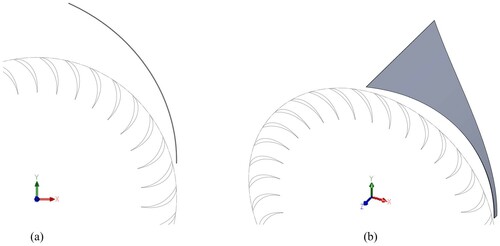
Figure 5. Section view on plane P. First, last and nth baffle profiles (solid black lines); fluid trajectories (dotted lines).

We require the direction of the inlet velocity at r = R_flap to be in the plane orthogonal to the turbine axis and the width w_b of the baffle at a larger distance R_max to be constant with respect to its position. We call this constant D_pipe. The resulting equation is also the equation of the distance of the nozzle walls along the turbine axis direction: (7) $w_b\left(r\right)=a{r}^2+br+c,$(7) where coefficients a, b and c are computed in order to satisfy the previous requirements by means of the following conditions:

1. w_b(R_flap) = W

2. w´_b(R_flap) = 0;

3. w_b(R_max) = D_pipe.

The profile of the nth baffle can also be written as function of the difference θ−θ_n, where θ_n is its rotation with respect to the first one (see Figure 5). The profile equation is (8) $\begin{array}{r}r\left(\theta -{\theta }_n\right)=R_e{\text{e}}^{\left(\theta -{\theta }_n\right)\tan \left(\alpha \right)}\iff {\theta }_n\le \theta \le {\theta }_n+{\theta }_{max}\end{array}$(8) where R_e = D/2, ${\theta }_{max}$is the maximum angle of the nth baffle with ${\theta }_n$ = 0 and ${\lambda }_{max}$is the maximum value of ${\theta }_n$ (see Figure 5). Observe that the first and last baffles are part of the nozzle wall and, except the first, the baffle profiles are cut for r < R_flap to allow rotation of the flap.

For large enough $\theta -{\theta }_n$ values, the velocity entering the channels between the baffles is very small, along with the local energy loss. D_pipe is computed in order to guarantee, in each point outside the baffle channels, a velocity always smaller than 1 m/s. The optimal number of baffles depends on λ_max and it is kept equal to 10 for λ_max equal to 90°. For a greater number of baffles, the friction forces in their channels become important. For a much smaller number of baffles the attack angle in the central part of their channels becomes much greater than the design value. In both cases, we get a relevant efficiency reduction.

The upper part of the nozzle, where the baffles are missing, is confined between the upper edge of the baffles (with r = R_max and w_b= D_pipe) and the external wall. At the inlet of the nozzle, for θ = θ_max  +  λ_max, the contour of the nozzle section must include the contour of the section of the inlet pipe. Moreover, to obtain an almost constant velocity outside the baffles in sections with different $\theta$ angles, we need to ‘cut’ the contour of the section adopted at the inlet section of the nozzle, with θ = θ_max  +  λ_max, for θ_max < θ < θ_max  +  λ_max. See the resulting shape of the external walls of the nozzle in Figure 6(a) compared to the external walls of the PRS in Figure 6(b). In H-PRS, the trace of the baffle edges is on a circular arc of radius R_max and the nozzle inlet section is the same SEC. A.

Figure 6. Shape of the nozzle external walls: (a) in H-PRS; and (b) in PRS.

Observe in Figure 6(a) that the upper wall of the nozzle for 0 < θ < θ_max is given by the first baffle and that the lower wall of the nozzle for λ_max < θ < λ_max + θ_max is given by the last one.

The profile r_c(θ−θ_max) of the upper nozzle wall (Figure 6(a)) has to satisfy the following conditions: r_c = R_max at θ  = θ_max, r_c = D_pipe + R_max at θ = θ_max +λ_max, the same slope of the initial baffle at θ = θ_max and the profile has to be orthogonal to the radius r_c at θ  = θ_max + λ_max. This can be obtained by setting: (9) $\begin{array}{rl}{r}_c\left(\theta -{\theta }_{max}\right)& =A(\theta -{\theta }_{max}{)}^3+B(\theta -{\theta }_{max}{)}^2\\ & +C\left(\theta -{\theta }_{max}\right)+D\end{array}$(9)

where coefficients A, B, C and D are computed in order to satisfy the following conditions:

1. $r_c\left({\lambda }_{max}\right)=R_{max}+D_{\text{pipe}}$

2. ŕ_c(λ_max) = 0;

3. r_c( 0 ) = R_max;

4. ŕ_c(0 ) = tan(α)R_max.

See sections of the entire proposed device in Figures 6 and 7.

Figure 7. Sections of the H-PRS turbine.

The optimal number of blades in cross-flow type turbines has been investigated by Sinagra et al. (2021).

In this case, we would expect the optimal n_b number of blades n_b to be larger, along with the optimal D_i/D ratio, because a significant amount of energy is also dissipated in the circular annulus holding the blades immediately after the runner inlet surface, owing to the small W value. By contrast, because a minimum thickness has always to be ensured for the blades, a much larger number of blades leads, in the tests carried out with the numerical model presented in the next section, to a larger energy dissipation, and the D_i/D and optimal n_b values remain equal, respectively, to 0.75 and 34 as previously estimated for the traditional PRS turbine.

5. The numerical model

5.1. Model description

The design criteria of the proposed device were tested using 3D Computational Fluid Dynamics (CFD), which allows quick simulation of a large number of different geometries. CFD is a powerful method for modeling various physical systems in order to predict the evolution of the governing state variables. This approach for solving engineering problems has recently gained importance owing to its effectiveness and applicability (Ramezanizadeh et al., 2019).

The numerical model adopted was solved using the ANSYS^® CFX commercial code, solving the Reynolds-Averaged Navier–Stokes (RANS) equations and parallel processing on several CPU Intel^® Xeon^® E5-2650 v3 machines. CFX, in the case of rotating machines, adopts a sliding mesh strategy (Ferziger & Peric, 2002), where the runner and its swept volume are discretized within a rotating reference system. This avoids the need for modeling the movement of the internal boundaries given by the surface of the runner blades, as in the cut-cell immersed boundary method (Ghalandari et al., 2019; Salih et al., 2019).

CFX gives the option of selecting one among different advection models. We chose the high-resolution scheme, which uses second-order differencing for the advection terms in flow regions with low variable gradients (Ceballos et al., 2017). The high-resolution scheme uses first-order advection terms in areas where the gradients change sharply, to prevent overshoots and undershoots, and maintain robustness. The RNG k–ϵ turbulence model was selected in the CFX code in accordance with previous studies (Ceballos et al., 2017; Sammartano et al., 2016; Sinagra et al., 2021); the interface between the stationary and rotating domains was of transient rotor–stator type. The root mean square residual was used for the convergence criterion with a residual target equal to 1.0 × 10⁻⁵. The same solver was used extensively in previous studies (Sinagra et al., 2020) and its results compared successfully with experimental laboratory and field data.

A flow rate equal to 50 l/s, head drop equal to 200 m and rotational velocity equal to 1000 rpm were taken as design data. According to the previous section, the resulting diameter D and width W are, respectively, 500 and 10 mm. The boundary conditions selected in the simulation according to the design data are the following: (a) the total pressure, corresponding to the piezometric level plus the kinetic energy per unit weight, at both the nozzle inlet and the outlet section of the casing; and (b) the rotational velocity of the runner. The initial condition for the transient flow simulation was the steady-state solution computed assuming a fixed runner and adding inertial and Coriolis forces.

5.2. Grid and time convergence analyses

A preliminary convergence analysis, carried out with steady-state simulations, was previously performed on the initial model of the H-PRS turbine in order to assess the optimal density of the mesh necessary to get a negligible numerical error with the minimum required computational time. Five different meshes were compared (Table 1). Figures 8 and 9 illustrate the four main zones of the domain: rotor, stator, blade and baffle surfaces. Figure 8 shows the mesh modeling the flow field inside the turbine, and the baffles as empty spaces. Figure 9 shows an external view of the turbine.

Figure 8. Section of grid scheme.

Figure 9. Trimetric view of grid scheme: (a) zoom on the front view of the runner in the radial direction; (b) zoom on the outlet section.

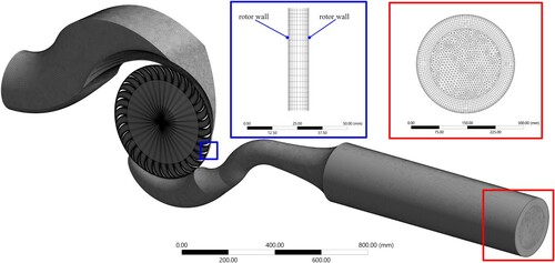
Table 1. Mesh parameters.

Mesh setting	Mesh 1	Mesh 2	Mesh 3	Mesh 4	Mesh 5
Rotor elements	4,428,228	6,270,348	8,727,936	10,824,240	12,752,397
Stator elements	6,243,046	9,090,586	11,595,911	13,983,856	16,734,099
Total elements	10,671,274	15,360,934	20,323,847	24,808,096	29,486,496

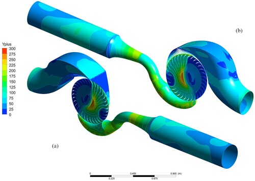
In the proximity of the blade surfaces, the baffle surfaces, the stator walls (Figure 8) and the rotor walls (Figure 9), the grids are highly clustered and the normalized distance y⁺ of the first-layer nodes from the impervious boundary is set in order to satisfy the literature requirements. In Figure 10, the computed y⁺ distribution is shown for the fourth mesh from two different observation points, one on the right (Figure 10(a)) and the other one on the left (Figure 10(b)) of the inlet pipe axis in the flow direction. We observe that the y⁺ values are always lower than 300, which satisfies the upper limit for the RNG k–ϵ turbulence model combined with a scalable wall function (Maduka & Li, 2021; Xu et al., 2021). With the exception of the blades that are not hit by the flow, all grid nodes satisfies also the lower limit given by 30 ≤ y⁺ (Maduka & Li, 2021).

Figure 10. Trimetric view of the y+ distribution from: (a) the right of the inlet section; (b) the left of the inlet section.

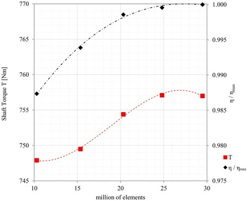
In Figure 11, the efficiencies η scaled with respect to the maximum efficiency η_max obtained with the fifth mesh, as well as the shaft torques computed with each mesh density, are shown plotted versus the corresponding number of elements. We observe a constant increment of the efficiency up to the fourth mesh, which is selected as the optimal one.

Figure 11. Shaft torque T and efficiency η scaled with respect to η_max versus the number of elements.

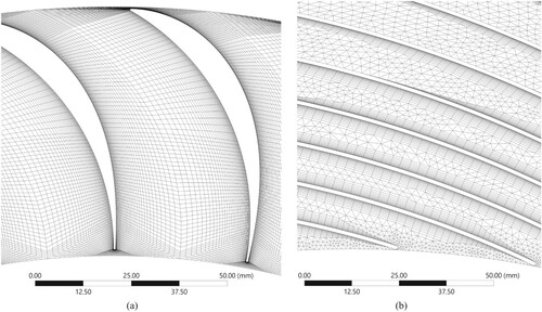
See details of the final convergence mesh: the blade zone in Figure 12(a) and the baffle zone in Figure 12(b).

Figure 12. Details of the convergence mesh: (a) blade zone; (b) baffle zone.

Some URANS analyses with the convergence mesh were also performed for the time-step-independence study. The number of time steps occurring per revolution of the runner and per each rotation angle between two blades of the same channel are shown in Table 2 for four different time step values. The maximum root mean square residual required to obtain a good convergence in each time step, usually achieved with 25 iterations (Xu et al., 2021), is set equal to 1.0 × 10⁻⁵.

Table 2. Parameters for time step-independence study.

	Time steps per	Number of time steps
Time step (s)	revolution	per channel
4.4 × 10^−4	136	4
2.9 × 10^−4	204	6
2.5 × 10^−4	238	7
2.2 × 10^−4	272	8

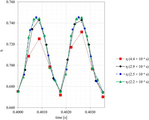
In order to guarantee periodic, deterministic convergence of the model, each analysis was run for a simulation time equal to 0.4 s, corresponding to more than six full revolutions (Sammartano et al., 2013; Sinagra et al., 2021). We observe in Figure 13 a constant reduction of the difference among the computed instantaneous efficiencies η(t) along with the time step reduction, up to a time step lower than 2.5 × 10⁻⁴ s, which is selected as the optimal one.

Figure 13. Efficiency versus time for different time steps.

6. H-PRS characterization

The numerical analysis was carried out by measuring the efficiency and the discharge of the turbine for each flap position and given net head (see Table 3), with an average computational time of 180 h per simulation. The flow rate changed in the range 8–54 l/s and the flap position changed in the range 22.5–90° of the runner inlet angle. The rotational velocity ω was assumed to be equal to 1000 rpm for all simulations. The test results are also shown in Figure 14. The curves show that the flap mobility makes it possible to save a constant net head for hydroelectric production within a large range of possible flow rates. Similarly, the flap position makes it possible to convey the sought-after flow rate by changing the head drop provided by the turbine. These characteristics of the turbine are essential for installations inside water supply networks.

Figure 14. H-PRS efficiency contour with the characteristic curve for each flap position.

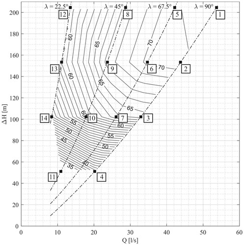
Table 3. Summary of the numerical analysis carried out to characterize H-PRS.

Simulation	λ (°)	ΔH (m)	Q (l/s)	η (%)
1	90	204.5	53.7	71.7
2	90	153.4	43.8	70.8
3	90	102.3	32.9	64.4
4	90	51.1	20.2	38.4
5	67.5	204.5	42.2	70.9
6	67.5	153.4	34.7	70.3
7	67.5	102.3	26.1	63.7
8	45	204.5	28.7	67.5
9	45	153.4	23.7	67.4
10	45	102.3	17.8	60.2
11	45	51.1	10.9	30.3
12	22.5	204.6	13.5	59.4
13	22.5	153.4	11.1	59.1
14	22.5	102.3	8.4	51.9

We observe in the iso-efficiency curves (Figure 14) that H-PRS shows the best efficiency equal to 71.7%, for a point close to the design data (Q_d = 50 l/s, ΔH_d = 200 m). For a large range of flow rates (20–54 l/s) and head drops (100–200 m) the efficiency reduction is lower than 10%. In the case of flow rates and head drops lower than 25% of design conditions, the curves show an abrupt reduction of efficiency. In these conditions, if the rotational velocity ω remains constant, the ratio between the inlet velocity V and the runner velocity is far from the optimal value V_r and dissipations grow drastically. In this case, the use of an inverter would provide great benefit. As example, for an a head drop equal to 50 m and a discharge equal to 20 l/s, the efficiency obtained by changing the rotational velocity from 1000 to 505 rpm to get the velocity ratio equal to 1.7 again is equal to 69.3% instead of the 38.5% value reported in the plot of Figure 14.

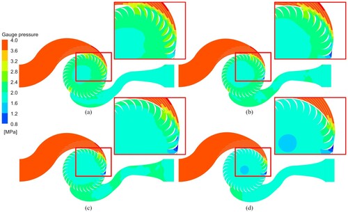
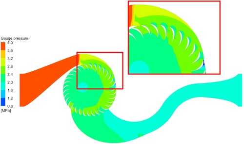
Figures 15 and 16 show, respectively, the velocity and the gauge pressure field at t = 0.4 s in the symmetry plane of the 3D transient simulations solved by assuming the design head drop for four different flap positions and corresponding values of the runner inlet angle λ. The results show that, owing mainly to the baffle-driven nozzle restriction, velocities sharply increase only around the runner inlet and outlet surface, where energy exchange occurs, and remain relatively low inside the nozzle, as well as in other parts of the runner, such as around the center, where they attain large values in traditional PRS turbines. The lowest pressure is reached close to the stator wall, immediately after the inlet surface in the rotation direction. This is probably due to the outlet flux of the corresponding channel, leading to a low pressure when the inlet flux is missing. This low pressure can provide cavitation, if the relative pressure in the outlet pipe is close to zero.

Figure 15. Velocity field in 3D transient simulation for different runner inlet angles: (a) λ = 90°; (b) λ = 67.5°; (c) λ = 45°; (d) λ = 22.5°.

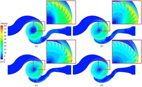
Figure 16. Gauge pressure field in 3D transient simulation for different runner inlet angles: (a) λ = 90°; (b) λ = 67.5°; (c) λ = 45°; (d) λ = 22.5°.

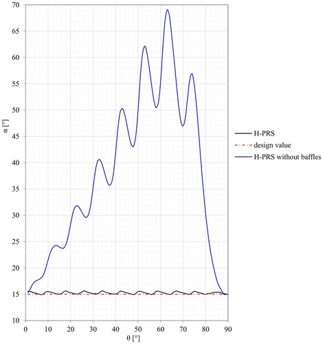
A very interesting result is also given by the two following tests. In the first one, the previously tested H-PRS turbine has been solved without the baffles inside the nozzle, resulting in a reduction of the efficiency from 71.7 to 46.5%. See in Figure 17 the profiles of the velocity inlet angle α for the case of a nozzle with baffles and without baffles at the same time t = 0.4 s, compared with the design value. When baffles are missing, a strong increment in the velocity inlet angle, much greater than the design one (15°), clearly resulting in a corresponding efficiency reduction. In the case with baffles, Figure 17 shows small periodical oscillations around the design value, with the valleys corresponding to the position of the baffles. In the case without baffles, the peaks of large periodical oscillations correspond to the position of the blades.

Figure 17. Velocity inlet angle α versus runner rotation angle θ (see Figure 6).

In the second test, a traditional PRS turbine has been solved assuming a fully open flap position. We can see that, in this case, we get a strong reduction of the total efficiency, from 71.7 to 53.7% (W/D ratio equal to 0.02 in Figure 2). The same traditional PRS, solved assuming free-slip boundary conditions on all the rigid walls, results in an efficiency equal to 78.5%. This suggests that the use of hydrophobic materials could be a valid alternative to the proposed H-PRS, if their use with high pressure fluids could guarantee long-term durability. Figures 18 and 19 show, respectively, the velocity and the gauge pressure field at t = 0.4 s in the symmetry plane of the 3D transient simulations solved, for traditional PRS and free-slip boundary conditions, by assuming the design head drop.

Figure 18. Velocity field in 3D transient simulation for traditional PRS, solved assuming free-slip boundary conditions.

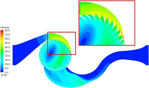
Figure 19. Gauge pressure field in 3D transient simulation for traditional PRS, solved assuming free-slip boundary conditions.

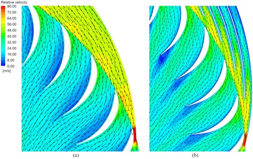
A comparison between Figures 18 and 15(a) shows that the average velocity of the fluid inside the nozzle in the case of traditional PRS is much higher than in case of H-PRS, due to the baffle restriction, but the velocity magnitude and the angle at the inlet surface of the runner are similar (see Figure 20, where the relative velocities are plotted in both the rotor and the stator domains). On the other hand, no-slip conditions on the baffle surface provide smaller velocities even close to the inlet surface of the runner, without any increment of their radial component. This suggests some energy dissipation in friction losses along the baffles, and a corresponding efficiency reduction (from 78.5 to 71.7%).

Figure 20. Relative velocity field near the impervious wall in: (a) traditional PRS assuming free-slip condition; and (b) H-PRS assuming no-slip condition.

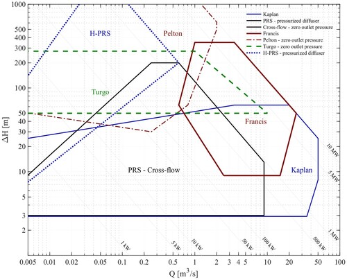
In Figure 21 we show that a turbine selection chart where the application field of H-PRS has been obtained by extending the original field of cross-flow turbines to the case of W/D smaller than 0.2. The original chart is taken from Sangal et al. (2013). The application field of H-PRS is shared by Pelton and Turgo turbines, but these need zero outlet pressure.

Figure 21. Turbine selection chart based on head and flow rate.

7. Conclusions

A new cross-flow type turbine, called H-PRS, has been proposed and tested numerically. The H-PRS turbine aims to fill a technological void that exists at the present time for hydropower production inside pipes where large head drops and small discharges are available, especially if the discharge has large temporal variability. The numerical results suggest fair efficiency of the proposed turbine for the design discharge, as well as an almost constant value for smaller discharge values, within a very large range. Optimization of the single machine parameters, including the diffuser shape and the rotational velocity, could also lead to further improvements. This research task is very hard to carry out because of the computational effort required by 3D solutions of complex meshes in transient conditions.

Much larger efficiencies can be attained by other turbines in the case of zero gauge pressure outlet discharge (Pelton) or low head drops and high discharge (Francis).

The results obtained by using the traditional PRS turbine assuming free-slip boundary conditions on all the rigid walls and the same runner geometry as adopted in the H-PRS suggest that most of the energy is lost in the new turbine by friction forces acting on the rigid walls. The development of new hydrophobic materials, at the present time still lacking the required long-term durability, could lead in the future to even more efficient and simple H-PRS turbines.

Notation

Cv	=	velocity coefficient (–)
D	=	outer runner diameter (m)
Di	=	inner runner diameter (m)
Dpipe	=	width of the baffle at a larger distance from the axis of the runner (m)
f	=	frequency of the AC grid (Hz)
g	=	acceleration due to gravity (m s–2)
nb	=	number of blades of the runner (–)
P	=	mechanical power produced (W)
p	=	number of polar couples of the electrical generator (–)
Q	=	water discharge rate (m3 s–1)
Qd	=	design water discharge rate (m3 s–1)
Re	=	outer runner radius (m)
Rflap	=	outer runner radius plus flap thickness (m)
Ri	=	inner runner radius (m)
Rmax	=	larger distance of the baffle from the axis of the runner (m)
r	=	distance r from the axis of the runner (m)
r  (θ−θn)	=	profile of the nth baffle (m)
rc  (θ−θmax)	=	profile of the upper nozzle wall (m)
Sc  (r)	=	area crossed by the water flow at a given distance r (m2)
V	=	inlet runner velocity (m s–1)
Vr	=	velocity ratio (–)
W	=	runner width at the outer diameter (m)
W(r)	=	runner wall distance in axial direction (m)
W*	=	maximum runner wall distance in axial direction (m)
wb (r)	=	distance of the nozzle walls along the turbine axis direction (m)
y+	=	normalized distance of the first layer nodes from the wall (–)
α	=	velocity inlet angle (radians or degrees)
γ	=	water specific weight (N m–3)
ΔH	=	specific energy drop per unit weigth (m)
ΔHd	=	design specific energy drop per unit weigth (m)
ε	=	flap thickness (m)
η	=	turbine efficiency (–)
ηmax	=	maximum H-PRS efficiency (–)
θ	=	generic angle of nth baffle (rad or degrees)
θmax	=	maximum angle of the first baffle (radians or degrees)
θn	=	nth baffle rotation with respect to the first one (radians or degrees)
λ	=	runner inlet angle (radians or degrees)
λmax	=	maximum inlet angle (radians or degrees)
ξ	=	specific energy drop coefficient (–)
ω	=	runner rotational velocity (rad s–1)

Disclosure statement

No potential conflict of interest was reported by the authors.

References

- Adhikari, R., & Wood, D. (2018). The design of high efficiency crossflow hydro turbines: A review and extension. Energies, 11(2), 267. https://doi.org/https://doi.org/10.3390/en11020267
- Algieri, A., Zema, D. A., Nicotra, A., & Zimbone, S. M. (2020). Potential energy exploitation in collective irrigation systems using pumps as turbines: A case study in Calabria (Southern Italy). Journal of Cleaner Production, 257, 120538. https://doi.org/https://doi.org/10.1016/j.jclepro.2020.120538
- Araujo, L. S., Ramos, H. M., & Coelho, S. T. (2006). Pressure control for leakage minimisation in water distribution systems management. Water Resources Management, 20(1), 133–149. https://doi.org/https://doi.org/10.1007/s11269-006-4635-3
- Carravetta, A., Del Giudice, G., Fecarotta, O., & Ramos, H. M. (2013). PAT design strategy for energy recovery in water distribution networks by electrical regulation. Energies, 6(1), 411–424. https://doi.org/https://doi.org/10.3390/en6010411
- Carravetta, A., Fecarotta, O., Sinagra, M., & Tucciarelli, T. (2014). Cost-Benefit analysis for hydropower production in water distribution networks by a pump as turbine. Journal of Water Resources Planning and Management, 140(6), 04014002. https://doi.org/https://doi.org/10.1061/(ASCE)WR.1943-5452.0000384
- Ceballos, Y. C., Valencia, M. C., Zuluaga, D. H., Del Rio, J. S., & García, S. V. (2017). Influence of the number of blades in the power generated by a Michell Banki turbine. International Journal of Renewable Energy Research, 7(4), 1989–1997. https://www.ijrer.org/ijrer/index.php/ijrer/article/view/6372/pdf
- Delgado, J., Ferreira, J. P., Covas, D., & Avellan, F. (2019). Variable speed operation of centrifugal pumps running as turbines. Experimental investigation. Renewable Energy, 142, 437–450. https://doi.org/https://doi.org/10.1016/j.renene.2019.04.067
- Dong, H., Cheng, M., Zhang, Y., Wei, H., & Shi, F. (2013). Extraordinary drag-reducing effect of a superhydrophobic coating on a macroscopic model ship at high speed. Journal of Materials Chemistry A, 1(19), 5886–5891. https://doi.org/https://doi.org/10.1039/C3TA10225D
- Fecarotta, O., Aricò, C., Carravetta, A., Martino, R., & Ramos, H. M. (2015). Hydropower potential in water distribution networks: Pressure control by PATs. Water Resources Management, 29(3), 699–714. https://doi.org/https://doi.org/10.1007/s11269-014-0836-3
- Ferziger, J. H., & Peric, M. (2002). Computational methods for fluid dynamics. Springer. ISBN 978-3-642-56026-2.
- Ghalandari, M., Bornassi, S., Shamshirband, S., Mosavi, A., & Chau, K. W. (2019). Investigation of submerged structures’ flexibility on sloshing frequency using a boundary element method and finite element analysis. Engineering Applications of Computational Fluid Mechanics, 13(1), 519–528. https://doi.org/https://doi.org/10.1080/19942060.2019.1619197
- Giudicianni, C., Herrera, M., Di Nardo, A., Carravetta, A., Ramos, H. M., & Adeyeye, K. (2020). Zero-net energy management for the monitoring and control of dynamically-partitioned smart water systems. Journal of Cleaner Production, 252, 119745. https://doi.org/https://doi.org/10.1016/j.jclepro.2019.119745
- Gupta, A., Bokde, N., Kulat, K., & Yaseen, Z. M. (2020). Nodal matrix analysis for optimal pressure-Reducing valve localization in a water distribution system. Energies, 13(8), 1878. https://doi.org/https://doi.org/10.3390/en13081878
- Kramer, M., Wieprecht, S., & Terheiden, K. (2017). Minimising the air demand of micro-hydro impulse turbines incounter pressure operation. Energy, 133, 1027–1034. https://doi.org/https://doi.org/10.1016/j.energy.2017.05.043
- Leman, O. Y., Wulandari, R., & Bintara, R. D. (2019). Optimization of nozzle number, nozzle diameter and number of bucket of pelton turbine using computational fluid dynamics and Taguchi methods. IOP Conference Series: Materials Science and Engineering, 694, 012017. https://doi.org/https://doi.org/10.1088/1757-899X/694/1/012017
- Maduka, M., & Li, C. W. (2021). Numerical study of ducted turbines in bidirectional tidal flows. Engineering Applications of Computational Fluid Mechanics, 15(1), 194–209. https://doi.org/https://doi.org/10.1080/19942060.2021.1872706
- Nakamura, Y., Komatsu, H., Shiratori, S., Shima, R., Saito, S., & Miyagawa, K. (2015). Development of high-efficiency and low-cost shroudless turbine for small hydropower generation plant. ICOPE 2015 - International Conference on Power Engineering Japan Society of Mechanical Engineers, Yokohama, Japan, 30 November 2015 through 4 December 2015. https://doi.org/https://doi.org/10.1299/jsmeicope.2015.12._ICOPE-15-_107.
- Nourhanm, S., Rawya, K., Walid, E., & Amr, F. (2017). Pressure control for minimizing leakage in water distribution systems. Alexandria Engineering Journal, 56(4), 601–612. https://doi.org/https://doi.org/10.1016/j.aej.2017.07.008
- Ramezanizadeh, M., Nazari, A. M., Ahmadi, M. H., & Chau, K. W. (2019). Experimental and numerical analysis of a nanofluidic thermosyphon heat exchanger. Engineering Applications of Computational Fluid Mechanics, 13(1), 40–47. https://doi.org/https://doi.org/10.1080/19942060.2018.1518272
- Rantererung, C. L., Tandiseno, T., & Malissa, M. (2019). Multi nozzle paralel to improve efficiency cross flow turbine. ARPN Journal of Engineering and Applied Sciences, 14(2), 550–555. http://www.arpnjournals.org/jeas/research_papers/rp_2019/jeas_0119_7588.pdf
- Salih, S. Q., Aldlemy, M. S., Rasani, M. R., Ariffin, A. K., Tuan Ya, T. M. Y. S., Al-Ansari, N., Yaseen, Z. M., & Chau, K. W. (2019). Thin and sharp edges bodies-fluid interaction simulation using cut-cell immersed boundary method. Engineering Applications of Computational Fluid Mechanics, 13(1), 860–877. https://doi.org/https://doi.org/10.1080/19942060.2019.1652209
- Sammartano, V., Aricò, C., Carravetta, A., Fecarotta, O., & Tucciarelli, T. (2013). Banki-Michell optimal design by computational fluid dynamics testing and hydrodynamic analysis. Energies, 6(5), 2362–2385. https://doi.org/https://doi.org/10.3390/en6052362
- Sammartano, V., Aricò, C., Sinagra, M., & Tucciarelli, T. (2015). Cross-flow turbine design for energy production and discharge regulation. Journal of Hydraulic Engineering, 141(3), 04014083. https://doi.org/https://doi.org/10.1061/(ASCE)HY.1943-7900.0000977
- Sammartano, V., Filianoti, P., Sinagra, M., Tucciarelli, T., Scelba, G., & Morreale, G. (2017a). Coupled hydraulic and electronic regulation of cross-flow turbines in hydraulic plants. Journal of Hydraulic Engineering, 143(1), 0401607. https://doi.org/https://doi.org/10.1061/(ASCE)HY.1943-7900.0001226
- Sammartano, V., Morreale, G., Sinagra, M., & Tucciarelli, T. (2016). Numerical and experimental investigation of a cross-flow water turbine. Journal of Hydraulic Research, 54(3), 321–331. https://doi.org/https://doi.org/10.1080/00221686.2016.1147500
- Sammartano, V., Sinagra, M., Filianoti, P., & Tucciarelli, T. (2017b). A Banki-Michell turbine for in-line hydropower systems. Journal of Hydraulic Research, 55(5), 686–694. https://doi.org/https://doi.org/10.1080/00221686.2017.1335246
- Samora, I., Hasmatuchi, V., Münch-Alligné, C., Franca, M. J., Schleiss, A. J., & Ramos, H. M. (2016). Experimental characterization of a five blade tubular propeller turbine for pipe inline installation. Renewable Energy, 95, 356–366. https://doi.org/https://doi.org/10.1016/j.renene.2016.04.023
- Sangal, S., Garg, A., & Kumar, D. (2013). Review of optimal selection of turbines for hydroelectric projects. International Journal of Emerging Technology and Advanced, 3(3), 424–830. https://ijetae.com/files/Volume3Issue3/IJETAE_0313_70.pdf
- Simão, M., & Ramos, H. M. (2019). Micro axial turbine hill charts: Affinity laws, experiments and CFD simulations for different diameters. Energies, 12(15), 2908. https://doi.org/https://doi.org/10.3390/en12152908
- Sinagra, M., Aricò, C., Tucciarelli, T., Amato, P., & Fiorino, M. (2019). Coupled electric and hydraulic control of a PRS turbine in a real transport water network. Water, 11(6), 1194. https://doi.org/https://doi.org/10.3390/w11061194
- Sinagra, M., Aricò, C., Tucciarelli, T., & Morreale, G. (2020). Experimental and numerical analysis of a backpressure Banki inline turbine for pressure regulation and energy production. Renewable Energy, 149, 980–986. https://doi.org/https://doi.org/10.1016/j.renene.2019.10.076
- Sinagra, M., Picone, C., Aricò, C., Pantano, A., Tucciarelli, T., Hannachi, M., & Driss, Z. (2021). Impeller Optimization in crossflow hydraulic turbines. Water, 13(3), 313. https://doi.org/https://doi.org/10.3390/w13030313
- Sinagra, M., Sammartano, V., Aricò, C., & Collura, A. (2016). Experimental and numerical analysis of a cross-flow turbine. Journal of Hydraulic Engineering, 142(1), 04015040. https://doi.org/https://doi.org/10.1061/(ASCE)HY.1943-7900.0001061
- Sinagra, M., Sammartano, V., Morreale, G., & Tucciarelli, T. (2017). A new device for pressure control and energy recovery in water distribution networks. Water, 9(5), 309. https://doi.org/https://doi.org/10.3390/w9050309
- Subekti, R. A., Susatyo, A., & Sudibyo, H. (2018, November 1–2). Design and analysis of crossflow turbine prototype for picohydro scale. International Conference on Sustainable Energy Engineering and Application (ICSEEA) Tangerang, Indonesia, pp. 1-2 November 2018. pp. 1–6. https://doi.org/https://doi.org/10.1109/ICSEEA.2018.8627139
- Vagnoni, E., Andolfatto, L., Richard, S., Münch-Alligné, C., & Avellan, F. (2018). Hydraulic performance evaluation of a micro-turbine with counter rotating runners by experimental investigation and numerical simulation. Renewable Energy, 126, 943–953. https://doi.org/https://doi.org/10.1016/j.renene.2018.04.015
- Xu, C., Fan, C., Zhang, Z., & Mao, Y. (2021). Numerical study of wake and potential interactions in a two-stage centrifugal refrigeration compressor. Engineering Applications of Computational Fluid Mechanics, 15(1), 313–327. https://doi.org/https://doi.org/10.1080/19942060.2021.1875887