Significant wave height forecasting using WRF-CLSF model in Taiwan strait

ABSTRACT

Short-term hourly reliable prediction of significant wave height is an important research topic in coastal engineering. Many researchers have carried out in-depth studies in many ocean regions. Generally, most of this work is implemented through numerical models. However, as for numerical models, with the increase of hourly prediction duration, the accumulation of wave randomness leads to the poor prediction effect. In this paper, four buoy stations in the Taiwan Strait are taken as the research objects. We propose a significant wave height prediction algorithm, which combines numerical weather prediction model WRF and deep-learning model, called WRF-CLSF(Convolution-LSTM-FC). WRF can forecast 24-h wind speed in real-time, based on a variety of interpretable physical mechanisms. CLSF aims to extract the information of historical wind-wave interaction scale and the trend of wind-wave coherence, with the help of convolution operation and the time series model(LSTM), respectively. In the experiment, the proposed model was compared with the state-of-the-art prediction model. The results show that WRF-CLSF has an outstanding prediction effect at four buoy observation stations along with the Taiwan Strait.

KEYWORDS:

• Significant wave height
• long short-term memory
• Taiwan strait
• WRF
• convolution neural network

1. Introduction

Ocean wave activities are closely related to people's life. The prediction of wave height in the coastal area affects many activities of coastal engineering, such as coastal protection engineering, marine traffic management, marine environmental monitoring, sediment movement research, ocean wave energy development, etc. Therefore, these marine applications put forward substantial requirements for the prediction of wave height, and many applications hope to get better continuous hourly prediction accuracy.

Because many factors affect the prediction of significant wave height, it is challenging to predict it continuously, hourly, and accurately (Deo & Naidu, 1998; Ro et al., 2020). Lots of existing researches use wave height characteristics to study the prediction work. These methods can be divided into the numerical modeling and the machine learning. The first one simulates the growth process of ocean waves through the fluid mechanism theory (Mosavi et al., 2019). This theory is relatively well developed, but it has high complexity and high computational overhead. Besides, the prediction effect is suboptimal. Therefore, as for the second one, Deo and Naidu (1998), libin et al. (2018), Shamshirband et al. (2020) and Wang et al. (2021) tried to use the machine learning method to make up for this deficiency. For example, libin et al. (2018) and Wang et al. (2021) used the time series network to learn the continuous dependency of the wind-wave for the prediction. These methods try to improve the prediction accuracy and the length of hourly lead times. In recent years, there are studies to find the prediction law from the characteristics and continuity of wind-wave. For example, Kambekar and Deo (2014) explored the relationship between historical wave characteristics and future wave height. Deka and Prahlada (2012) attempted to study the prediction from the combination method of wave decomposition and neural network. Ali and Prasad (2019) relies on the influence of wind and the wind-wave continuity characteristics to study the prediction. However, the inherent information of the wind-wave itself has not been fully extracted. There are still some problems, such as the short duration of hourly prediction and low prediction accuracy.

Another challenge of significant wave height prediction is that the main influencing factors will change due to different geographical environments. The geographical environment of the Taiwan Strait is relatively special, and the wave height in the offshore area is affected by many factors, such as wave refraction and diffraction, water depth, swell and shallow wave, etc. Tingting et al. (2010) among which the wind force plays a leading role. However, Taiwan island faces mainland across the sea, when the sea breeze passes by, it leads to the ‘narrow tube effect’ (Guoling & Hanqiu, 2019). This leads to a certain lag of the wave. That is to say, the wave height will not immediately react with the wind field passing through. However, the hysteresis did not affect the subsequent sharp change of wave height. Given this special environment, libin et al. (2018), Wang et al. (2021) and Yan et al. (2012) have carried on the research and done the summary to the forecasting of this ocean area. Among them, there are widely used numerical prediction methods (Yan et al., 2012). However, the actual prediction results of most studies are suboptimal. Therefore, the prediction of significant wave height in the Taiwan Strait should also depend on the internal interaction of wave and wind field, as well as the continuous change trend after the combined effect of wind and wave.

The difficulty of significant wave height prediction also lies in the randomness and instability of sea wave (Hou et al., 2012). Lei et al. (2010), Nitsure et al. (2012), and Peres et al. (2015) tried to find a solution to overcome the difficulty. The most direct idea is to use the future wind field information to suppress the problems (Nitsure et al., 2012). But in practical application, it is impossible to know the accurate wind field information in advance. Therefore, Lei et al. (2010) and Peres et al. (2015) used the future wind field forecasted by the numerical model to predict the significant wave height. However, the forecasted wind fields used in these studies are not targeted enough. (Peres et al., 2015) Using the wind field at different positions, there was no accurate wind field information at each buoy. In (Lei et al., 2010), the time interval of using wind field is large, and the wind field information is sparse in time. Therefore, these are limitations to reduce the randomness and instability of ocean waves.

To solve the above problems, we propose WRF-CLSF model to predict the significant wave height in the offshore area of the Taiwan Strait. The model features with hourly prediction ability of significant wave height in the next 24 h. Besides, it considers the interaction scale of wind wave and wind field, as well as the trend of wind-wave coherence. This model, combined with WRF numerical weather prediction model algorithm (Abdelwares et al., 2017), effectively suppresses the randomness and instability of sea waves. The model has the ability to extract the information of historical measured information, as well as the ability to learn wind-wave sequence in the time dimension.

The main contributions of this article are as follows:

• At present, most of the research oceans are generally stable, while the sea conditions of the Taiwan Strait are complex. There are few researches about the prediction along with the Taiwan Strait. Our research put forward a good reference method.

• Most deep-learning methods are based on past wind field or wave height data for analysis or prediction. Our proposed model integrating the WRF prediction algorithm which considers the geographical and meteorological factors, effectively suppresses the randomness and instability of sea waves.

• In this study, we designed a method to extract the interaction scale information of wind waves and predict the coherence information of the wind-wave in time. It provides a good reference for the prediction of significant wave height.

• In most coastal wave height studies, the duration of continuous hourly prediction is relatively short. The hourly prediction duration in this study is up to 24 h, which provides a good reference for real-time hourly prediction.

The remaining structure of this article is as follows: The second part introduces the research progress of wave height prediction. The third part introduces the framework of WRF-CLSF model in detail. The experimental results and discussion are in the fourth part. The fifth part summarizes the research, the limitations of the model, and the prospects.

2. Related work

The prediction of significant wave height is a challenging problem in the marine field. Mainly, in term of methods, there are two categories, including numerical modeling and machine learning.

2.1. Numerical modeling

Numerical modeling, based on the fluid mechanics, is a kind of traditional research method, which has experienced a long-time development. The commonly applied numerical models are WAVEWATCH III (Tolman & Chalikov, 1996), MRI-iii (Kohno & Tsukuba-Shi, 2004), SWAN (Booij et al., 1999). Among them, the SWAN is a widely used offshore wave simulation method, which introduces many factors and uses the concept of the large and small grid in space. SWAN model has been applied in the Black Sea (Akpinar et al., 2012), Gulf of Southern California (Rogers et al., 2007), and Beaufort Sea area (Azharul Hoque et al., 2020) to study the prediction. de León et al. (2018) compared and analyzed the performance of SWAN and WAVEWATCH III in predicting wave height in the North Sea of Europe. Without exception, SWAN model is also applied in the coastal areas of the Taiwan Strait (Chenkemin et al., 2019). However, it is caused the suboptimal result in the complex sea area such as Taiwan Strait, because of a large amount of calculation, long prediction time, and the random deviation accumulation. Therefore, it is necessary to find other stable methods to predict the significant wave height more accurately.

2.2. Machine learning

Compared with the numerical model, the machine learning method is devoted to data statistical analysis to forecast significant wave height and has less computation. The support vector machine (Etemad-Shahidi & Mahjoobi, 2009), KNN, regression tree (Mahjoobi & Etemad-Shahidi, 2008), fuzzy inference system (Cornejo-Bueno et al., 2018), and other methods are used to study the prediction. And the short-term prediction result is significantly better than the numerical model. Since neural network emerged, Deo and Naidu (1998) and Londhe and Panchang (2006) has adopted this technology with the relationship between the historical and the future to forecast the next four moments. But there are some problems, for example, the number of prediction lead times is short, the prediction time interval is large, and the factors considered are simple. In recent years, Ali et al. (2020), Berbić et al. (2017) and Nitsure et al. (2012) have taken several influencing factors into account. For example, Ali et al. (2020) considered the historical values, maximum values, period, sea surface temperature, and other factors to study the prediction work, but the prediction duration is only half an hour. Nitsure et al. (2012) added the wind field information to predict the next three moments values. Berbić et al. (2017) also considered the wind field data for the prediction research, and the hourly prediction duration is up to 11 h. In the above studies, with the increase of hourly prediction, the accuracy decreases. Few studies have been able to predict more than 12 h continuously.

In recent years, Ali and Prasad (2019), Deka and Prahlada (2012), Duan et al. (2016) and Ni and Ma (2020) combined machine learning method with a decomposition of sea wave observations to predict significant wave height. For example, Ali and Prasad (2019) combined extreme learning machine with empirical value decomposition to forecast the future height. Duan et al. (2016) combined empirical value decomposition with support vector machine for prediction. Deka and Prahlada (2012) combined wavelet decomposition with the neural network for prediction work. Ni and Ma (2020) used the principal component analysis to predict the wave height in the polar region. Many studies using wave decomposition show that different factors will affect the future wave height trend. Firstly, the duration of wind-wave interaction is a crucial factor in forming significant wave height. However, since the parameters of the wave decomposition method are not unique, it is difficult to get better settings. Secondly, wind and wave have a certain scale of coherence in time, which affects the smoothness in a certain time range. These two factors have an important influence on the prediction work.

In recent years, with the in-depth development of machine learning, deep learning has become an important development direction (Ghalandari et al., 2019; Yafouz et al., 2021; Yaseen et al., 2020; Zeinalzadeh & Pakatchian, 2021). Deep learning optimizes the model parameters through the data-driven mechanism. Such as convolutional neural network(CNN), recurrent neural network(RNN), long-term memory network(LSTM) (Hochreiter & Schmidhuber, 1997), gate control unit(GRU) (Chung et al., 2014), and other models have been widely used in time series information learning. For example, Liu et al. (2019) proposed WaveNet model based on CNN network to evaluate the prediction performance on simulated datasets. It indeed shows that the CNN network has an excellent ability to extract wind and wave interactions. In recent years, researchers have applied the LSTM model (libin et al., 2018), and GRU model (Wang et al., 2021) to study the prediction in the coastal waters of Taiwan Strait. And, Ni and Ma (2020) also used the LSTM model to study the prediction in polar regions. From the above analysis, it shows that the LSTM model is a feasible approach for the prediction work. Still, the multi-dimensional output information of the LSTM model cannot sufficiently describe the future wave height characteristics. It can only roughly describe its time trend. In fact, it can only describe the coherence trend of the wave in the future.

To improve the prediction accuracy, some researchers begin to take wind messages into account for the prediction work. For example, Nitsure et al. (2012) added the measured wind information to conducting the post prediction research on the coast of North America and the Indian Ocean. However, it is impossible to get accurate wind information in advance in practical application. Peres et al. (2015) used The NCEP / NCAR reanalysis wind field to is used to supplement the missing data over the years. This study uses the numerical model to forecast the wind speed information every 6 h. The wind speed information interval is longer, and the wind information does not match the buoy position in space, so the wind-wave coherence continuity information is less. It is difficult to predict the future wave height in the future because the continuous information and continuity of wind cannot be accurately obtained to a great extent. Therefore, the prediction needs stable and continuous wind field information to suppress the randomness and instability of ocean waves.

To solve the above problems, this paper proposes WRF-CLSF model to predict the hourly significant wave height of the Taiwan Strait in the next 24 hours. The model combines with the WRF weather forecast model to predict the wind speed to suppress the randomness of ocean waves. At the same time, the model uses the powerful feature extraction method to extract continuity and interaction scale from the wind-wave historical information. Because it is difficult to obtain the continuous hourly measured wave height, wind speed, and the WRF model detail message from other ocean area, this paper only studies the significant wave height prediction of four stations in the Taiwan Strait.

Compared with other prediction methods, the main advantage of our method is that it features with the data-fitting ability of deep learning and the comprehensive advantages of the WRF in geographical environment, spatial, and time state. Thus, the model provides strong support for the accuracy of hourly 24-hour prediction. The advantages and limitations of current significant wave height prediction methods are summarized in Table 1.

Table 1. The main advantages of the proposed system over existing methods and its limitations.

Model	Advantages	Limitations
Numerical modeling	Fully developed theory,	Lots of calculation,
	Strong explanatory,	Complex implementation,
	Configurable ability	Suboptimal application effect
Traditional machine learning	Widely used,	Short hourly prediction,
	Strong classification ability	Not ideal prediction accuracy
Machine learning based on wave decomposition	Multiscale acquisition of wave characteristics,	Uncertain decomposition scale,
	the prediction effect is certainly improved	Difficult to determine the scale in different sea areas
Deep learning	Good time series learning ability.	Short hourly prediction,
		Insufficiently to extract the wind-wave message
WRF-CLSF	Strong wind-wave feature extraction,	The peak significant wave height is underestimated,
	Feasible suppression of wind-wave randomness,	The prediction effect of extreme wave height is insufficient.
	relatively long hourly prediction

3. Methodology

In this part, we mainly introduce the composition of the WRF-CLSF model. The first part is WRF (weather research and forecasting model). The second part is CLSF(Convolution-LSTM-FC). The specific model structure is shown in Figure 1.

Figure 1. Flowchart of the WRF-CLSF network model.

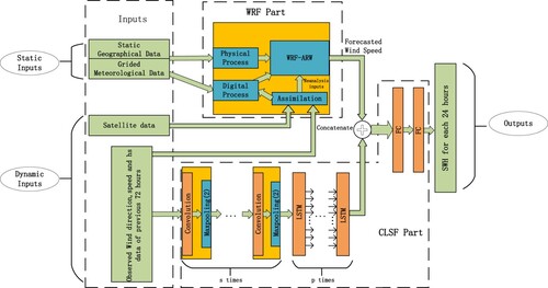
3.1. WRF method

The numerical weather forecast model (WRF) is a new generation of mesoscale weather forecast model and assimilation system, which is widely used in the weather forecast. WRF has two kind dynamic frameworks, WRF-ARW and WRF-NMM, respectively, which correspond to research mode and business mode. WRF-ARW is used in this paper. The model includes numerical filtering process, physical process, and dynamic process. The physical process uses static geographical data Get and meteorological information Met to simulate atmospheric motion. This process also needs a parametric optimization scheme opti to get a more reasonable control quality. The physical process is described as follows: (1) $\begin{array}{rl}& physica{l}_{-}process=physica{l}_{-}op(Geo,Met)\end{array}$(1) (2) $\begin{array}{rl}& optimized=optimizatio{n}_{-}op\left(physica{l}_{-}process\right)\end{array}$(2) In this study, the GFS global spectral model of the National Center for Environmental Prediction (NCEP) was used to assimilate the initial background field and the lateral boundary of the large grid, according to satellite meteorological data Sat and observed wind speed information. The NCEP-GFS initialization method has been compared and analyzed in Carvalho et al. (2014). The simplified assimilation process is as follows: (3) $assimulate{d}_{-}data=NCE{P}_{-}GFS(Sat,observe{d}_{-}wind)$(3) The role of the numerical filtering process is to filter the interference information of the assimilation data and the measured data to enhance the effectiveness of the initial field data (Shu-chang et al., 2008) The specific process is as follows: (4) $\begin{array}{rl}& filtere{d}_{-}data\\ & =digita{l}_{-}filte{r}_{-}op(assimulate{d}_{-}data,Geo,Met)\end{array}$(4) The assimilated input data and atmospheric motion process are used in the dynamic process. The Euler equation is used to solve the process. Specifically, from the vertical direction, it is divided into 23 layers. The η has the following definition: (5) $\begin{array}{r}\eta =\frac{p_h-p_{ht}}{\mu }\end{array}$(5) Where $\mu =p_{hs}-p_{ht}$, $p_{ps}$ and $p_{ht}$ is the pressure of the surface and the upper boundary, so $0\le \eta \le 1$. The Euler formula of WRF-ARW dynamic process can be expressed as: (6) $\begin{array}{rl}& \frac{\mathrm{\partial }U}{\mathrm{\partial }t}+(\mathrm{\nabla }\cdot V_u)-\mu \alpha \frac{\mathrm{\partial }p}{\mathrm{\partial }x}+\left(\frac{\alpha }{{\alpha }_d}\right)\frac{\mathrm{\partial }}{\mathrm{\partial }\eta }\left(\frac{\mathrm{\partial }p}{\mathrm{\partial }\eta }\frac{\mathrm{\partial }\varphi }{\mathrm{\partial }x}\right)=F_U\end{array}$(6) (7) $\begin{array}{rl}& \frac{\mathrm{\partial }V}{\mathrm{\partial }t}+(\mathrm{\nabla }\cdot V_v)-\mu \alpha \frac{\mathrm{\partial }p}{\mathrm{\partial }y}+\left(\frac{\alpha }{{\alpha }_d}\right)\frac{\mathrm{\partial }}{\mathrm{\partial }\eta }\left(\frac{\mathrm{\partial }p}{\mathrm{\partial }\eta }\frac{\mathrm{\partial }\varphi }{\mathrm{\partial }y}\right)=F_V\end{array}$(7) (8) $\begin{array}{rl}& \frac{\mathrm{\partial }W}{\mathrm{\partial }t}+(\mathrm{\nabla }\cdot V_w)-g\left[\left(\frac{\alpha }{{\alpha }_d}\right)\frac{\mathrm{\partial }p}{\mathrm{\partial }\eta }-{\mu }_d\right]=F_W\end{array}$(8) (9) $\begin{array}{rl}& \frac{\mathrm{\partial }W}{\mathrm{\partial }t}+\frac{\mathrm{\partial }\theta }{\mathrm{\partial }t}+(\mathrm{\nabla }\cdot V_{\theta })=F_{\theta }\end{array}$(9) (10) $\begin{array}{rl}& \frac{\mathrm{\partial }\mu }{\mathrm{\partial }t}+(\mathrm{\nabla }\cdot V)=0\end{array}$(10) (11) $\begin{array}{rl}& \frac{\mathrm{\partial }\varphi }{\mathrm{\partial }t}+\frac{1}{\mu }(\mathrm{\nabla }\cdot V_{\varphi }-gW)=0\end{array}$(11) (12) $\begin{array}{rl}& \frac{\mathrm{\partial }{Q}_m}{\mathrm{\partial }t}+(\mathrm{\nabla }\cdot V_{qm})=F_{Q_m}\end{array}$(12) Among them, ϕ is potential force, F is external force, μ is friction factor, θ is temperature level, $q_m$ 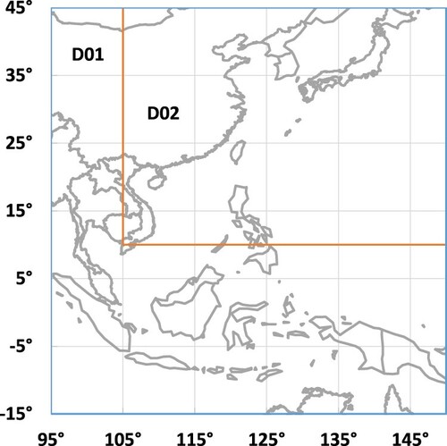is unit humidity. The model contains three-dimensional spatial information. Specifically, the coarse grid is used in a large area, and the nested grid is used in a specific research area. In space, the coarse grid of the study area is Asia and the Northwest Pacific, with a regional range of ${95}^{\circ }E\sim {150}^{\circ }E$, ${15}^{\circ }S\sim {45}^{\circ }N$, and a horizontal resolution of ${0.5}^{\circ }$. The inner nested fine grid is the sea area around the Taiwan Strait, with a range of ${105}^{\circ }E\sim {150}^{\circ }E$, ${10}^{\circ }N\sim {45}^{\circ }N$, and the horizontal resolution is ${0.2}^{\circ }$. As shown in Figure 2.

Figure 2. Study area of WRF model.

The simplified algorithm of WRF is as follows:

3.2. CLSF method

3.2.1. Historical information extraction

Because the significant wave height is mainly affected by the wind speed, and the different directions of wind also have a great impact on the significant wave height. The growth of sea waves is closely related to the continuous action of wind. Therefore, wind direction, wind speed, and significant wave height are used as input data in the wind-wave information extraction method. The significant wave height in the next 24 h is affected by the continuous inertia of the wave itself and the reflection of the seabed topography and the surrounding coastline. Therefore, we consider using the 72-hour measured significant wave height, wind speed and wind direction as the basis for extracting these information. We use h for the significant wave height, p for wind speed, and d for wind direction. Before using these three data sets, we normalized the observed data to accelerate the convergence of feature extraction. The specific operation is as follows: (13) $\begin{array}{r}{X}_{norm}=\frac{X-X_{min}}{X_{max}-X_{min}}\end{array}$(13) The interaction between wind and wave determines the primary extraction length on the three components. We have the following definition for the information extraction process of wind-wave action scale, where k represents the length of one extraction: (14) $\begin{array}{r}\begin{array}{rl}{h}_k\left(t\right)& =h[t,t+k]\\ p_k\left(t\right)& =p[t,t+k]1\le t\le l-k\\ d_k\left(t\right)& =d[t,t+k]\end{array}\end{array}$(14) The data input involves two major factors: the measured significant wave height and the wind field. The wind speed in the Taiwan Strait has a unique narrow tube effect, so the velocity of the waves will also be accelerated theoretically. Therefore, we set up a multiple feature extraction operation, known as convolution operation, to extract the interaction information of significant wave height and wind field in time. We define three vectors groups of parameters ${\omega }_h$, ${\omega }_p$, ${\omega }_d$, to represent the linear combination of significant wave height, wind speed, and wind direction in each extraction process. We also define a constant vector to achieve the purpose of nonlinear operation, represented by $b_k$. We define the following matrix operations: (15) $\begin{array}{r}{f}_k\left(t\right)=[{\omega }_h,{\omega }_p,{\omega }_d]\cdot \left[h_k\right(t),p_k(t),d_k(t\left)\right]+b_k\end{array}$(15) In general, the matrix operation can be performed many times, resulting in the output: $\left[f_{k_1}^1\right(t),f_{k_2}^2(t),\dots f_{k_n}^n(t\left)\right]$. Where n represents the n times of extracting the interaction scale of wind-wave information. The output ${f_{k_n}^n\left(t\right)}_1$ is n groups of output after the first feature extraction operation. After getting the output ${f_{k_n}^n\left(t\right)}_1$, we divide the output into n/2 groups continuously and do the maximum selection operation on each group of extracted information to obtain the salient features. Specifically, for any n, we can get $f_{k_n}^n\left(t\right)$, and we perform the following maximum value selection operation: (16) $\begin{array}{r}{f}_{m,k_n}^n\left(t\right)=max\left\{f_{k_n}^n\right(t),f_{k_n}^n(t+1\left)\right\},1\le t\le \frac{l-k}{2}\end{array}$(16) Thus, the groups of outputs $\left\{f_{m,k_n}^n\right(t){\}}_1$ can be obtained after the maximum value operation, where m represents the maximum value selection operation flag. After obtaining the output, the next feature extraction is carried out to further extract the wind-wave interaction scale information. The calculation process is as described in the previous formula. After s-step feature extraction, the result $\left\{f_{m,k_n}^n\right(t){\}}_s$ is obtained. After feature extraction, the output can be regarded as a multi-dimensional expression of the wind and waves on time $\mathbf{t}$.

The prediction of significant wave height is essentially a continuous inertial prediction process of wind-wave interaction. But this coherence is influenced by many factors. Therefore, before the final significant wave height prediction, obtaining the wind-wave continuous information is necessary. We use the dimension information of wind-wave interaction after s-step feature extraction $\left\{f_{m,k_n}^n\right(t){\}}_s$, and use long-term and short-term memory network (LSTM) to predict the continuous information. Specifically, the first LSTM coherence prediction process of wind-wave information is as follows: (17) $\begin{array}{r}\begin{array}{rl}{X}_t& =\left\{f_{m,k_n}^n\right(t){\}}_s\\ S\left(0\right)& =Random\left(t\right)\\ S\left(t\right),O\left(t\right)& =LST{M}_1({\omega }_f^1,{\omega }_i^1,{\omega }_c^1,{\omega }_o^1,S(t-1),X_t)\end{array}\end{array}$(17) Where $S\left(0\right)$ is the initial random information, and $X_t$ is the extracted dimension information of wind-wave action at t time. ${\omega }_f$,${\omega }_i$,${\omega }_c$, and ${\omega }_o$ are the parameter of LSTM, which represents the forgetting gate, input gate, status gate and output gate, respectively. After the first LSTM process, the intermediate output of $\left[O\right[1],O[2],\dots O(t\left)\right]$ is obtained. Further, LSTM prediction operation is performed on the intermediate output of the previous LSTM, this operation carries out $\mathbf{p}\mathbf{-}\mathbf{1}$ times, and the specific operation is as follows: (18) $\begin{array}{rl}S\left(t\right),H{S}_e\left(t\right)& =LST{M}_{p-1}({\omega }_f^{p-1},{\omega }_i^{p-1},{\omega }_c^{p-1},{\omega }_o^{p-1},\\ & S(t-1),O\left(t\right))\end{array}$(18) Where ${\omega }_f^{p-1}$, ${\omega }_i^{p-1}$, ${\omega }_c^{p-1}$, and ${\omega }_o^{p-1}$ are the parameters of the p-th LSTM. We take $h{s}_e=last\left\{H{S}_e\right(t\left)\right\}$ as the coherence prediction information of wind and wave in the future. $h{s}_e$ has 24 dimensions.

3.2.2. Fusion prediction

We fuse the wind speed information predicted by WRF with the wind-wave coherrence prediction value to get the fused information $H{s}_{\tau }$. The specific operation is as follows: (19) $\begin{array}{r}H{s}_{\tau }=V_{fore}\oplus h{s}_e\end{array}$(19) $H{s}_{\tau }$ not only has the characteristics of the WRF forecasting data, but also has the information characteristics of historical significant wave height and wind field. Finally, two-layer adaptive neural network (FC) is used to predict the final significant wave height. The specific operation is as follows, where W and B are the learning parameters of the neural network: (20) $\begin{array}{r}\begin{array}{rl}h{s}_{\sigma }& =H{s}_{\tau }\cdot W_1+B_1\\ hs& =h{s}_{\sigma }\cdot W_2+B_2\end{array}\end{array}$(20) The simplified algorithm of CLSF is as follows:

3.2.3. Activation and loss function

At present, there are many activation functions, including sigmoid and tanh. The values of sigmoid and tanh functions are in the range of $0\sim 1$ and $-1\sim 1$, respectively, and their absolute values are less than 1. The continuous gradient operation after multi-layer training is prone to gradient disappearance. And they have a certain computation, compared with the ReLU activation function, which will slow down the model calculation speed. The family of ReLU activation functions includes ReLU function, leaky ReLU function, parameter ReLU (P-ReLU) activation function, and so on. Among them, the parameters in the P-ReLU function can be trained. Therefore, this activation function is more conducive to the expression of nonlinearity (Xu et al., 2015). So we use the P-ReLU function as the activation function. In this study, most activation functions are the P-ReLU, as Equation (21(21) $\begin{array}{r}f\left(x\right)=\left\{\begin{array}{ll}0,& x\le 0\\ \alpha x,& x>0\end{array}\right.\end{array}$(21) ) shown. (21) $\begin{array}{r}f\left(x\right)=\left\{\begin{array}{ll}0,& x\le 0\\ \alpha x,& x>0\end{array}\right.\end{array}$(21) The loss function used for training is MSE. MSE has the advantages of convenient calculation, accurate measurement error, and good convergence effect, as shown in Equation (22(22) $\begin{array}{r}Loss=MSE=\frac{1}{m}\sum _{i=1}^m[H{S}_{obs}^{\left(i\right)}-H{S}_{pre}^{\left(i\right)}].\end{array}$(22) ). We use the ADAM algorithm to optimize gradient descent (Kingma & Ba, 2014). (22) $\begin{array}{r}Loss=MSE=\frac{1}{m}\sum _{i=1}^m[H{S}_{obs}^{\left(i\right)}-H{S}_{pre}^{\left(i\right)}].\end{array}$(22)

4. Experiment

In this experiment, we evaluated the performance among the proposed WRF-CLSF network, some classical time series forecasting models, and numerical method.

4.1. Datasets

The research data are taken from the wave height observation devices of Fujian Marine Forecasts in the Taiwan Strait. The Taiwan Strait is an important transportation hub connecting the East China Sea and the South China sea, whose wave and weather phenomena are complex. The positions of the specific buoy observation stations are shown in Figure 3.

Figure 3. Locations of the four buoys in the Taiwan Strait.

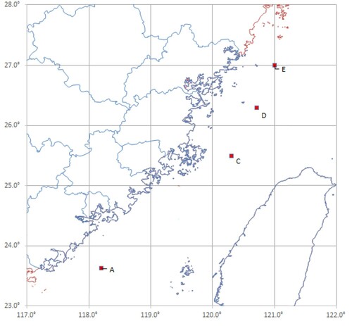
Because of the large amount of missing data at station B, we focuses on the significant wave height prediction from other four stations. We used the measured data of the four stations in 2016, 2017, and 2019 for the prediction research. Due to the lack of all buoy observation data in 2018, we do not take the data into account for our study. This study uses the 2016 data to train, the 2017 data to verify, and the 2019 data to test. We use 2017 data to select the super parameters for deep-learning models and use 2019 data to compare and analyze the prediction performance for each model.

In this research, our prediction interval is 1 hour. In each interval, we forecast the next 24-hour significant wave height continuously. For deep-learning sample sets. We obtain the sample details in the form of table, shown as Table 2.

Table 2. Samples detail for deep-learning models.

Sample type	Items	Station A	Station C	Station D	Station E
Training	Missing days	0	34	0	0
	Samples	8665	7753	8665	8665
Validation	Missing days	0	0	73	98
	Samples	8665	8665	6814	6218
Test	Missing days	0	67	94	27
	Samples	8665	8570	6576	7396

Although the location of C, D and E stations is relatively close, their data is missing for a certain period. Moreover, their missing data complement each other. To completely analyze the prediction effect in this area, we studied these three stations. Most of the observed information in other sea areas only has significant wave height data, no matching wind field information. Moreover, most of the available observation information is missing. The WRF parameters information about other ocean areas needed in this study is difficult to obtain from other research institutions. Therefore, this study does not involve the prediction in other sea areas.

According to the information of buoy equipment from the Fujian Marine Forecasts, the significant wave height below 0.6 m belongs to the equipment initialization or maintenance status. Specifically, the statistical information of the wind-wave information of the four stations is shown in Table 3.

Table 3. Statistical information of wind speed and significant wave height at the four research sites.

	Wind speed (m/s)					Wave Height(m)
Station	Average	Max	Std	Skewness	Kurtosis	Average	Max	Std	Skewness	Kurtosis
A	7.78	25.5	4.72	0.36	−0.91	1.59	6.1	1.09	0.87	0.01
C	8.53	31.1	4.41	0.18	−0.67	1.69	7.7	1.12	0.87	0.35
D	8.30	25.6	4.04	0.12	−0.57	1.55	8.5	0.98	1.02	1.16
E	7.62	21.1	3.83	0.20	−0.62	1.20	6.4	0.68	1.33	2.92

From Table 3, we can obtain that the average wave heights of the C and D stations are higher than those of other stations, and the wind speed is the same case. However, compared to the wave weight, the wind-speed distribution is relatively flat. From station E to station A, the wind speed intensity increases; however, this trend is not followed by the wave height.

4.2. Evaluation indexes

We evaluate the performance of our model using the MSE, RMSE, MAE, $R^2$, standardized deviation(sstd), and model prediction correlation coefficient(R), where MSE has already been defined previously. We use the Taylor diagram to show the comprehensive performance between the predicted and observed values.

Taylor diagram is mainly used to evaluate the prediction performance of the regression model. Given two sets of data, $f_n$ and $r_n$, we define $\overline{f}$ and $\overline{r}$ as the mean values of two groups of data, define ${\sigma }_f$ and ${\sigma }_r$ as the standardized variances of the two data groups, and define R as the correlation coefficient of the two groups of data. The specific calculation method of R shown in formula 29(29) $\begin{array}{rl}& R=\frac{\sum _{i=1}^m\left(H{S}_{pre}^{\left(i\right)}-\overline{H{S}_{pre}}\right)\left(H{S}_{obs}^{\left(i\right)}-\overline{H{S}_{obs}}\right)}{\sqrt{\sum _{i=1}^m{\left(H{S}_{pre}^{\left(i\right)}-\overline{H{S}_{pre}}\right)}^2\sum _{i=1}^m{\left(H{S}_{obs}^{\left(i\right)}-\overline{H{S}_{obs}}\right)}^2}}.\end{array}$(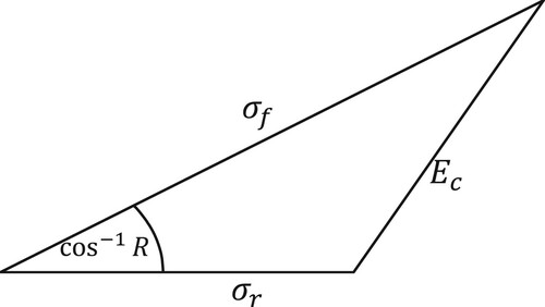29) . Taylor diagram defines the following calculation method: (23) $\begin{array}{r}{E}_c^2={\sigma }_f^2+{\sigma }_r^2-2{\sigma }_f{\sigma }_{r}R\end{array}$(23) Where $E_c$ is the centralized RMSE value, and the specific calculation is shown as follows: (24) $\begin{array}{r}{E}_c=\sqrt{\frac{1}{N}\sum _{n=1}^N\left[\right(f_n-\overline{f})-(r_n-\overline{r}){]}^2}\end{array}$(24) Formula 23(23) $\begin{array}{r}{E}_c^2={\sigma }_f^2+{\sigma }_r^2-2{\sigma }_f{\sigma }_{r}R\end{array}$(23) similar to the cosine theorem, is shown in the Figure 4.

Figure 4. Taylor calculation principle.

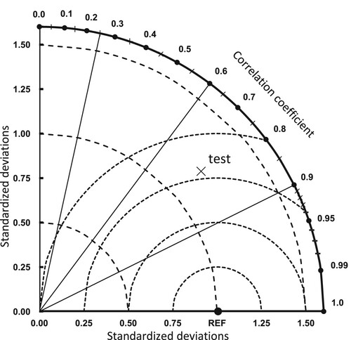
In order to compare the performance of the model conveniently, the Tayler diagram standardizes the above statistical data. The specific method is to divide the statistics by the standardized variance($\widehat{E_c}=E_c/{\sigma }_r$, $\widehat{{\sigma }_f}=\sigma /{\sigma }_f$, $\widehat{{\sigma }_r}=1$). Where $\widehat{E_c}$ is the standard deviation, as shown in formula 28(28) $\begin{array}{rl}& sstd=\frac{\sqrt{\frac{1}{m}\sum _{i=1}^m{\left(H{S}_{pre}^{\left(i\right)}-\overline{H{S}_{pre}}\right)}^2}}{\sqrt{\frac{1}{m}\sum _{i=1}^m{\left(H{S}_{obs}^{\left(i\right)}-\overline{H{S}_{obs}}\right)}^2}}.\end{array}$(28) . So, we get the Tayer evaluation diagram as Figure 5.

Figure 5. Taylor evaluation diagram.

Other specific performance evaluation indexes are as follows: (25) $\begin{array}{rl}& RMSE=\sqrt{\frac{1}{m}\sum _{i=1}^m{\left(H{S}_{obs}^{\left(i\right)}-H{S}_{pre}^{\left(i\right)}\right)}^2}.\end{array}$(25) (26) $\begin{array}{rl}& MAE=\frac{1}{m}\sum _{i=1}^m∣H{S}_{obs}^{\left(i\right)}-H{S}_{pre}^{\left(i\right)}∣.\end{array}$(26) (27) $\begin{array}{rl}& R^2=1-\frac{\sum _{i=1}^m\left(H{S}_{obs}^{\left(i\right)}-H{S}_{pre}^{\left(i\right)}\right)}{\sum _{i=1}^m\left(\overline{H{S}_{obs}}-H{S}_{obs}^{\left(i\right)}\right)}.\end{array}$(27) (28) $\begin{array}{rl}& sstd=\frac{\sqrt{\frac{1}{m}\sum _{i=1}^m{\left(H{S}_{pre}^{\left(i\right)}-\overline{H{S}_{pre}}\right)}^2}}{\sqrt{\frac{1}{m}\sum _{i=1}^m{\left(H{S}_{obs}^{\left(i\right)}-\overline{H{S}_{obs}}\right)}^2}}.\end{array}$(28) (29) $\begin{array}{rl}& R=\frac{\sum _{i=1}^m\left(H{S}_{pre}^{\left(i\right)}-\overline{H{S}_{pre}}\right)\left(H{S}_{obs}^{\left(i\right)}-\overline{H{S}_{obs}}\right)}{\sqrt{\sum _{i=1}^m{\left(H{S}_{pre}^{\left(i\right)}-\overline{H{S}_{pre}}\right)}^2\sum _{i=1}^m{\left(H{S}_{obs}^{\left(i\right)}-\overline{H{S}_{obs}}\right)}^2}}.\end{array}$(29) where $H{S}_{obs}$ is the observed significant wave height, $H{S}_{pre}$ is the significant wave height predicted by the models, and m is the predicted hours.

4.3. Comparison algorithm

In this experiment, we compare the results of several significant models to illustrate the performance of the proposed CLSF model. These models include deep-learning models and numerical models. The models based on deep-learning include BP, LSTM, GRU and the WRF-CLSF model proposed in this paper.

Comparison of existing time series deep-learning models:

• BP (Shamshirband et al., 2020): Back propagation neural network. It is the most widely used network model in the field of significant wave height prediction. Because of its strong nonlinear fitting ability, it can express almost any mapping relationship. In the experiment, we use the historical wind-wave data to predict the future significant wave height.

• LSTM (libin et al., 2018): The long short-term memory network is a widely used time series prediction model. In the actual prediction, the model is usually established following by a neural network. In the experiment, we use the historical wind-wave data to predict the significant wave height.

• GRU (Wang et al., 2021): The gate recurrent network is a simplified version of LSTM, and its operating speed is fast. Researchers have also studied the significant wave height of the Taiwan Strait using this network model.

Comparison with traditional numerical models:

• SWAN (Chenkemin et al., 2019): Numerical modeling of coastal shallow-water waves. It is a widely used numerical model in ocean research,

The deep-learning model proposed in this research:

• WRF-CLSF: Combined with the WRF model algorithm, it has the ability to extract wind-wave interaction information and coherence information. The model is explained in detail in the previous sections.

4.4. Parameter setting

The SWAN is the production of the operational numerical prediction system of Fujian Marine Forecasts, which is the forecasting department of the Taiwan Strait and surrounding waters. The dual bidirectional grid-nesting technology is adopted. The coarse grid includes Asia and the Northwest Pacific, with a regional range of ${95}^{\circ }E\sim {150}^{\circ }E$ and ${15}^{\circ }S\sim {45}^{\circ }N$, with a horizontal resolution of ${0.5}^{\circ }$. The internal nested fine grid is the sea area around the Taiwan Strait, with a regional range of ${105}^{\circ }E\sim {150}^{\circ }E$ and ${10}^{\circ }N\sim {45}^{\circ }N$, with a horizontal resolution of ${0.2}^{\circ }$. The wave model runs in an OpenMPI parallel environment.

In the deep-learning experiment, we use the following hardware environment: Two GeForce GTX1080TI and two GeForce GTX2080TI, the memory capacity is 64GB. The software environment is Ubuntu 16.04 LTS, python 3.5, and TensorFlow 2.0-GPU. The general experimental parameters of the deep-learning model are as follows: most deep-learning models use the same activation function P-ReLU. The learning rate of the Adam optimizer is 0.001, the number of training iterations is 500, and the dropout rate is 0.2.

We use the greedy strategy to optimize the parameters of the deep-learning model. Specifically, the first step is to select a better number of model layers, and the second step is to select better model parameters through multiple experiments.

The optimization of the BP model parameters: as the number of layers increases, the fitting effect of the model becomes worse. So, in the first step, we set up a 1 to 10 layer BP model, 10 experiments in total, marked as BP-1 to BP-10, in which the number of neurons is 24, this group of experiments can get the best number of BP hidden layers. Experiments show that BP-2 and BP-3 have good results in the verification dataset. Second, we try to find a better combination of neuron parameters. The number of neurons in the last layer is always 24 due to predicting the continuously 24-hourly significant wave height. Therefore, we set the number of neurons as 12, 16, 20, 28, 32, 36, 40, 44, and 48. The second experiment found better parameters through the combination of parameters, 37 experiments in total. Through the parameter search, we know that BP-2 is better than BP-3 in general, and BP-2 has a better prediction effect on the validation set when the first layer neurons are 36 and the second are 24. Here we use BP-2-36-24 to represent the model.

The optimization of the LSTM model parameters: BP model parameters optimization results show that the number of the model layer should not be too many, and the same case as the neuron. Therefore, in the first step, we designed three experiments to obtain the optimal number of LSTM layers. The LSTM layers of the first, the second and the third experiment are set with 2, 3 and 4, respectively, and 24 neurons were set in each layer, and the ANN layer with 24 neurons was set at the end of each LSTM model. Based on the first step, we get that the two-layer LSTM model has a good prediction effect on the validation set, expressed by LSTM-2. We set 26, 28, 30, 32, 34, 36, and 38 neuron numbers for LSTM-2 and carried out 21 experiments to obtain the optimal number of neurons. The experiment shows that the neuron parameter of two-layer LSTM is 24, which has a good effect. We marked it as LSTM-2-24.

The optimization of the GRU model parameters: From the optimization results of LSTM, we can see that the number of GRU layers is set to two. First, we set the number of neurons in the second layer as 24, and then we optimize the neurons number in the first layer. We set up 12, 16, 18, 22, 26, 30, 34, 38, 42, 46 neurons in the second layer, 10 experiments in total. Finally, the experiment shows that when the number of neurons in the first layer is 24, the effect is better. We marked it as GRU-2-24.

Optimization of WRF parameters for WRF-CLSF model: The parameters optimization of WRF involves many optimization schemes of fluid mechanics. By comparing the observed values, we obtained the model suitable for the meteorological forecast of the Taiwan Strait. From the results of wind field prediction, we get the message that: With the increase of forecast time, the error is increasing. Therefore, we choose the continuously 24-hourly model algorithm to forecast wind speed.

Optimization of CLSF parameters for WRF-CLSF model: According to parameter optimization of BP model and LSTM model, CLSF model chooses two-layer LSTM and two-layer FC model. For the parameter optimization of wind-wave interaction feature extraction, we also use the greedy strategy. The wind-wave feature extraction process is determined by the extraction length k and the linear combination scale n, In the first step, we set up three experiments, the first extracted once, the second extracted twice, and the third extracted three to get the best feature extraction times s. Specifically, we set 9,7 for K and N, respectively, and get the better results of the two extraction processes. In the second step, we use k1, n1, and k2, n2 to represent the parameters of the two extraction processes and set them to 3, 5, 7, 9, 11, 13, 15, and carry out combination training. Finally, we get the WRF-CLSF parameters: continuously 24-Hourly wind field parameters of WRF. Two-layer convolution operation information extraction process of CLSF model, where k1 = 9, n1 = 3, k2 = 7, n2 = 5. Two-layer LSTM, each layer includes four gate structures and each gate structure has 24 neurons. The last two layers are the FC layer, whose neurons in the first layer are 36, in the second are 24.

The specific parameters of each model are shown in Table 4. The l is the number of hidden layers, $h_i$ is the number of neurons in the ith hidden layer, g is the learning rate, and p is the number of training times. $K_i$ is the extraction length of the ith layer convolution operation, and $N_i$ is the number of ith layer convolution operations.

Table 4. Detailed parameter description of each model.

Algorithm	Component	Settings
BP-2-36-24	BP	l=2,h1=36,h2=24, activation=PReLU,p=500,g=0.001	p=500,g=0.001
LSTM-2-24	LSTM	l=2,h1=24,h2=24,activation=tanh	p=500,g=0.001
	ANN	l=24,activation=PReLU
GRU-2-24	GRU	l=2,h1=24,h2=24,activation=tanh,	p=500,g=0.001
	ANN	l=24,activation=PReLU
SWAN
	Doublenesting grids, Coarse lo: ${95}^{\circ }-{150}^{\circ }E$, la :15${}^{\circ }S-{45}^{\circ }N$, Horizontalresolution: 0.5${}^{\circ }$, Fine lo:105${}^{\circ }-{150}^{\circ }E$; la :10${}^{\circ }-{45}^{\circ }N$, Horizontal resolution 0.2${}^{\circ }$, wind inputs, Wave Shoaling, Diffraction, Bottom friction, Wave breaking, Whitecap, Wave-wave nonlinear interaction
WRF-CLSF	WRF
		Version: 3.7.1, integration step:180s, Double nesting, coarse-mesh-accuracy:60 km,coarse-mesh-accuracy:20 km, Microphysical parameter scheme: WSM6 Hail, Near surfacelayer scheme: Monin-Obukhov, Land surface process scheme: Noah, Boundary layerscheme: YSU, Boundary layer parameterization: Shallow Kain-Fritsch(newEta)
	CLSF	Convoluation: layer=2, k1=9,n1=3,k2=7,n2=5, activation=PReLU LSTM:layer=2, neurons of each=24 FC: layer=2, first layer neuron=36, second layerneuron=24, activation=PReLU	p=500,g=0.001

5. Performance comparison

We compare all models' performance using the characteristics of buoys and the results of each model for each buoy.

5.1. Analysis in terms of space

It can be concluded from Table 5 that the prediction effect of the WRF-CLSF model is obviously better than other models at four different sites from west to East. We can tell that the error indices (RMSE, MSE, MAE) of all models in the site E are smaller, but the determination coefficient $R^2$ is worse than other sites. This feature can be obtained by comparing and analyzing the forecast results and wind speed data. The mean and extreme wind speed near the surface are relatively weak at site E, and the significant wave height is generally low. And we can notice that the wind speed standard deviation is low, and the coefficient of determination of model fitting results is not high.

Table 5. Each model performance of forecasting significant wave height above 0.6 m.

Model	Metric	Station A	Station C	Station D	Station E
BP-2-36-24	mse	0.48	0.43	0.29	0.22
	rmse	0.70	0.65	0.54	0.48
	mae	0.47	0.48	0.38	0.33
	$R^2$	0.49	0.43	0.56	0.36
LSTM-2-24	mse	0.47	0.36	0.25	0.18
	rmse	0.68	0.60	0.50	0.42
	mae	0.46	0.42	0.35	0.28
	$R^2$	0.51	0.53	0.61	0.48
GRU-2-24	mse	0.39	0.34	0.26	0.19
	rmse	0.62	0.58	0.51	0.44
	mae	0.41	0.40	0.34	0.29
	$R^2$	0.60	0.56	0.61	0.47
SWAN	mse	0.40	0.30	0.36	0.23
	rmse	0.62	0.55	0.60	0.49
	mae	0.58	0.41	0.46	0.35
	$R^2$	0.58	0.61	0.46	0.34
WRF-CLSF	mse	0.18	0.19	0.17	0.11
	rmse	0.43	0.43	0.42	0.33
	mae	0.32	0.33	0.30	0.24
	$R^2$	0.81	0.75	0.74	0.69

From the analysis of the scatter diagram, as shown in Figure 6, the significant wave height of site E is significantly lower than that of other sites, and the fitting result of site A is better than that of other sites. Compared with the numerical model, SWAN, the prediction effect of the deep learning models are more concentrated. The SWAN considers the spatial and wave dynamic factors. Moreover, the initial boundary conditions greatly influence the prediction results. The deep-learning models need to adapt to the specific wave situation. Different wave environments need models with different parameters to train for forecasting significant wave height.

Figure 6. Scatter diagram of the prediction effect of all models at all observation stations. (a) Relationship of BP-2-36-24 for four stations, (b) Relationship of LSTM-2-24 for four stations, (c) Relationship of GRU-2-24 for four stations, (d) Relationship of SWAN for four stations, (e) Relationship of WRF-CLSF for four stations.

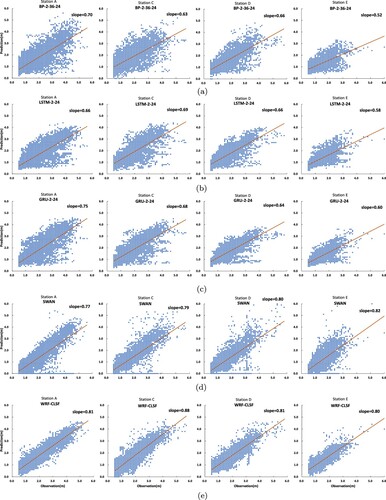
From the Figure 6, we read that the significant wave heights of site A and C are larger, while the site D and E are smaller. The results of LSTM-2-24 and GRU-2-24 are generally poor. The prediction result of SWAN is generally low. At the same time, the prediction of the SWAN at site E is relatively scattered. In general, the WRF-CLSF model is better than other models in forecasting the four sites.

5.2. Analysis from different significant wave height

To further analyze the prediction effect, we get the performance result of models forecasting the measured data greater than 1.5 m and 2.0 m, as shown in Table 6 and 7, respectively. From Table 4, we get that the WRF-CLSF model is still superior to other benchmark models. Specifically, the performance of other models is quite different from that of WRF-CLSF. The $R^2$ of LSTM-2-24 and BP-2-36-24 above 1.5 m at four stations is negative, and the prediction ability is poor. The SWAN model can predict the significant wave height above 1.5 m for site A and site C, but the indexes (MSE, RMSE, MAE) are quite different from WRF-CLSF, so the prediction effect is not ideal. From Table 5, compared with other models, WRF-CLSF model has better performance in predicting significant wave height above 2.0 meters. Specifically, the indexes (MSE, RMSE, MAE) of LSTM-2-24 and BP-2-36-24 models are quite different from those of WRF-CLSF model. The prediction ability index $R^2$ of the WRF-CLSF model is positive in stations A, C, and D, which has a certain prediction effect. From the prediction results of different heights, the prediction effect of the numerical model and deep-learning models gradually weakened with the increase of predicted wave height. The errors of indexes (MSE, RMSE, MAE) are increasing, while the value of the determination coefficient $R^2$ is decreasing. All models show that the higher the significant wave height is, the weaker the prediction ability is.

Table 6. Each model performance of forecasting significant wave height above 1.5 m.

Model	Metric	Station A	Station C	Station D	Station E
BP-2-36-24	mse	0.72	0.56	0.49	0.51
	rmse	0.85	0.75	0.70	0.72
	mae	0.61	0.55	0.52	0.54
	$R^2$	−0.10	−0.16	−0.07	−0.13
LSTM-2-24	mse	0.74	0.51	0.40	0.41
	rmse	0.86	0.72	0.63	0.64
	mae	0.62	0.51	0.44	0.47
	$R^2$	−0.12	−0.07	−0.03	−0.85
GRU-2-24	mse	0.58	0.47	0.43	0.45
	rmse	0.75	0.68	0.66	0.67
	mae	0.54	0.48	0.46	0.50
	$R^2$	0.14	0.02	0.07	−0.10
SWAN	mse	0.55	0.43	0.57	0.45
	rmse	0.74	0.66	0.75	0.67
	mae	0.60	0.50	0.60	0.49
	$R^2$	0.14	0.13	−0.19	−0.89
WRF-CLSF	mse	0.25	0.22	0.28	0.20
	rmse	0.49	0.48	0.53	0.44
	mae	0.39	0.36	0.40	0.34
	$R^2$	0.62	0.52	0.38	0.09

Table 7. Each model performance of forecasting significant wave height above 2.0 m.

Model	Metric	Station A	Station C	Station D	Station E
BP-2-36-24	mse	0.94	0.71	0.70	0.90
	rmse	0.97	0.84	0.83	0.95
	mae	0.70	0.62	0.63	0.76
	$R^2$	−0.87	−0.93	−0.95	−3.16
LSTM-2-24	mse	0.97	0.68	0.57	0.74
	rmse	0.98	0.83	0.75	0.86
	mae	0.73	0.60	0.53	0.68
	$R^2$	−0.94	−0.87	−0.60	−2.46
GRU-2-24	mse	0.72	0.62	0.62	0.81
	rmse	0.85	0.79	0.79	0.90
	mae	0.61	0.55	0.56	0.72
	$R^2$	−0.44	−0.70	−0.75	−2.73
SWAN	mse	0.62	0.51	0.71	0.64
	rmse	0.78	0.71	0.85	0.80
	mae	0.62	0.55	0.66	0.60
	$R^2$	−0.24	−0.33	−0.92	−1.82
WRF-CLSF	mse	0.31	0.24	0.35	0.28
	rmse	0.55	0.49	0.60	0.53
	mae	0.44	0.37	0.45	0.43
	$R^2$	0.38	0.33	0.01	−0.32

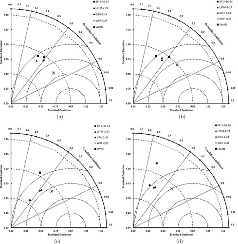
From the Tayler diagram of the four buoys, as shown in Figure 7, it can be seen that the sign of the WRF-CLSF model is closest to the reference point (REF) among the four locations. LSTM-2-24 is close to GRU-2-24, and has a similar prediction effect, but their prediction effect is weaker than WRF-CLSF at four stations. In general, the prediction performance of WRF-CLSF is better than that of the numerical model and other deep-learning models.

Figure 7. Taylor performance maps for all baseline models at all observation points. (a) Station A Talyer diagram, (b) Station C Talyer diagram, (c) Station D Talyer diagram, (e) Station E Talyer diagram.

5.3. Peak significant wave height prediction analysis

Here, we further analyze the relative error of significant wave height above 2 m. From Table 8, the prediction relative error of the WRF-CLSF model above 2 m is significantly smaller than that of the SWAN numerical model and other deep-learning models. The relative error of the LSTM-2-24 model at the four stations is relatively large, which indicates that only using the LSTM model or the GRU to predict significant wave height is not good enough. In contrast, the relative error of the WRF-CLSF model is less than 9%, which indicates that the WRF meteorological prediction algorithm model and convolution feature extraction algorithm have a positive effect on significant wave height prediction.

Table 8. The all models prediction relative error more than 2.0 m at all observation stations(%).

Model	Station A	Station C	Station D	Station E
BP-2-36-24	13.28	12.36	10.06	9.68
LSTM-2-24	12.71	11.76	10.63	10.44
GRU-2-24	11.86	11.58	10.21	9.36
SWAN	12.50	11.57	11.28	8.46
wrf-CLSF	8.26	8.28	8.09	6.15

In order to further analyze the difference in peak prediction between the SWAN model and the WRF-CLSF model, two of which use the forecasted wind speed information, and we get the results as shown in Figures 8–11.

Figure 8. SWAN and WRF-CLSF outputs at station A.

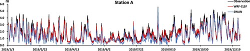
Figure 9. SWAN and WRF-CLSF outputs at station C.

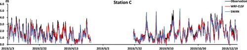
Figure 10. SWAN and WRF-CLSF outputs at station D.

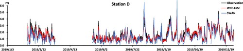
Figure 11. SWAN and WRF-CLSF outputs at station E.

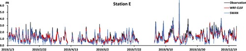
From the prediction effect at all stations, the result of the SWAN model for higher peak value is not much different from that of the WRF-CLSF model, but the lower significant wave height is underestimated. Site C, site D and site E are close to each other, but they all have some missing values. According to the observed wave heights of station D and station E in June, the fluctuation of significant wave heights of station C is not too dramatic, and the prediction effect of the WRF-CLSF in Station C is more stable than that of the SWAN. From the observation data of site C and site D in August, we inferred that the significant wave height of site E will appear peak and low values, and the prediction effect of the WRF-CLSF model is also better. The WRF-CLSF has a better prediction effect in the whole year.

We further analyze the influence of the wind field information of WRF weather forecast on the prediction effect. The measured wind speed, wind direction, and the correlation coefficient between wind speed and wave height at the four observation stations are shown in Figures 12–15.

Figure 12. Wind speed, wind direction, and the correlation coefficient between significant wave height and wind speed at station A. (a) Winter, (b) Spring, (c) Summer, (d) Autumn, (e) Wind speed and wave height correlation coefficient in station A.

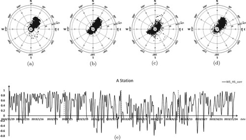
Figure 13. Wind speed, wind direction, and the correlation coefficient between significant wave height and wind speed at station C. (a) Winter, (b) Spring, (c) Summer, (d) Autumn, (e) Wind speed and wave height correlation coefficient in station C.

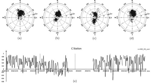
Figure 14. Wind speed, wind direction, and the correlation coefficient between significant wave height and wind speed at station D. (a) Winter, (b) Spring, (c) Summer, (d) Autumn, (e) Wind speed and wave height correlation coefficient in station D.

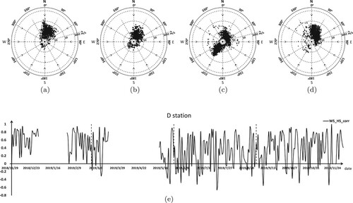
Figure 15. Wind speed, wind direction, and the correlation coefficient between significant wave height and wind speed at station E. (a) Winter, (b) Spring, (c) Summer, (d) Autumn, (e) Wind speed and wave height correlation coefficient in station E.

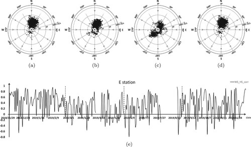
We can see that the monsoon feature of all sites is obvious. The wind direction and speed at all stations in summer features with central symmetry, and the distribution of the southwest and the northeast wind is relatively balanced. The Pearson correlation coefficient(WS_HS_CORR) of wind speed and significant wave height fluctuates dramatically through the whole year. This shows that the wind field is not the decisive factor for the significant wave height prediction. However, the prediction result of the models with no future wind message, such as LSTM-2-24, BP-2-36-24, is not as good as WRF-CLSF. From the seasonal view, the monsoon characteristics in winter and autumn are more obvious, the wind direction is mainly from northeast to southwest, and the wind speed is faster. However, the correlation coefficient (WS_HS_CORR) fluctuates greatly, which indicates that convolution operation has a positive impact on extracting the interaction between wind field and significant wave height. As well as the more common typhoon weather in summer, convolution can also play a certain effect.

From the above analysis, we can see that the prediction effect of the WRF-CLSF model is better than other existing time series prediction models, and is also better than SWAN, the numerical model, combined with wind field prediction. The monsoon characteristics of the four buoy stations in the Taiwan Strait are obvious. The WRF-CLSF model, which combines the convolution operation to extract the interaction and the function to forecast the continuous characteristics, has a good performance in predicting the continuously 24-hour significant wave height at four sites.

6. Conclusions

In the complex coastal environment of Taiwan Strait, the SWAN model cannot get good prediction results. Through the comparison and analysis, we can see that the WRF-CLSF model is better than other models. From the prediction results of LSTM-2-24 and GRU-2-24 models, we conclude that using the time series prediction method simply is not enough. And from the results of the BP-2-24 model, we get that only considering the historical message is also not enough. And, it is necessary to introduce the future continuous 24-hour wind speed information to predict the significant wave height in the future. Finally, we conclude that the WRF-CLSF model has a good advantage in continuously predicting significant wave height in the next 24 h.

Limitations: WRF-CLSF underestimates the prediction of higher significant wave height. Therefore, the effect of the WRF-CLSF prediction on extreme wave height is insufficient. In future research, we will focus on combining the advantages of the numerical model and deep-learning method for the peak prediction accuracy.

The future research directions are as follows: under the current promise effect of current real-time hourly prediction, the peak prediction accuracy will be improved. Efforts should be made to explore other methods to extract more interactions between waves and the regional environments through deep learning. In order to enhance the accuracy of the forecast, we should try to obtain other forecast information about WRF in other sea areas.

Disclosure statement

No potential conflict of interest was reported by the author(s).

Additional information

Funding

This research was funded by Fujian Provincial Marine Economy Development Special Fund Project [grant number ZHHY-2019-02].

References

- Abdelwares, M., Haggag, M., Wagdy, A., & Lelieveld, J. (2018). Customized framework of the WRF model for regional climate simulation over the Eastern NILE basin. Theoretical and Applied Climatology, 134(3-4), 1135–1151. https://doi.org/https://doi.org/10.1007/s00704-017-2331-2
- Akpinar, A., Vledder, G. P. V., & ÖZger, M. (2012). Evaluation of the numerical wave model (SWAN) for wave simulation in the Black sea. Continental Shelf Research, 50-51(C4), 80–99. https://doi.org/https://doi.org/10.1016/j.csr.2012.09.012
- Ali, M., & Prasad, R. (2019). Significant wave height forecasting via an extreme learning machine model integrated with improved complete ensemble empirical mode decomposition. Renewable and Sustainable Energy Reviews, 104, 281–295. https://doi.org/https://doi.org/10.1016/j.rser.2019.01.014
- Ali, M., Prasad, R., Xiang, Y., & Deo, R. C. (2020). Near real-time significant wave height forecasting with hybridized multiple linear regression algorithms. Renewable and Sustainable Energy Reviews, 132, 110003. https://doi.org/https://doi.org/10.1016/j.rser.2020.110003
- Azharul Hoque, M., Perrie, W., & Solomon, S. M. (2020). Application of SWAN model for storm generated wave simulation in the Canadian beaufort sea. Journal of Ocean Engineering and Science, 5(1), 19–34. https://doi.org/https://doi.org/10.1016/j.joes.2019.07.003
- Berbić, J., Ocvirk, E., Carević, D., & Lončar, G. (2017). Application of neural networks and support vector machine for significant wave height prediction. Oceanologia, 59(3), 331–349. https://doi.org/https://doi.org/10.1016/j.oceano.2017.03.007
- Booij, N., Ris, R. C., & Holthuijsen, L. H. (1999). A third generation model for coastal regions-1. Model description and validation. Journal of Geophysical Research Atmospheres, 104, 7646–7666. https://doi.org/https://doi.org/10.1029/98JC02622
- Carvalho, D., Rocha, A., Gómez-Gesteira, M., & Silva Santos, C. (2014). WRF wind simulation and wind energy production estimates forced by different reanalyses: Comparison with observed data for Portugal. Applied Energy, 117, 116–126. https://doi.org/https://doi.org/10.1016/j.apenergy.2013.12.001
- Chenkemin, T., Xianchang, Y., Xiongbin, W., Shaohua, W., Qihua, H., & Lan, Z. (2019). Impacts of wind data on the hindcast of wave height simulated by SWAN model on the Taiwan strait. Acta Oceanologica Sinica, 41(5), 59–69.
- Chung, J., Gulcehre, C., Cho, K., & Bengio, Y. (2014). Empirical evaluation of gated recurrent neural networks on sequence modeling.
- Cornejo-Bueno, L., Rodríguez-Mier, P., Mucientes, M., Nieto-Borge, J., & Salcedo-Sanz, S. (2018). Significant wave height and energy flux estimation with a genetic fuzzy system for regression. Ocean Engineering, 160, 33–44. https://doi.org/https://doi.org/10.1016/j.oceaneng.2018.04.063
- de León, S. P., Bettencourt, J., Vledder, G. P. V., Doohan, P., & Dias, F. (2018). Performance of WAVEWATCH-III and SWAN models in the North sea. ASME 2018 37th International Conference on Ocean, Offshore and Arctic Engineering, Madrid, Spain. American Society of Mechanical Engineers, U.S.
- Deka, P. C., & Prahlada, R. (2012). Discrete wavelet neural network approach in significant wave height forecasting for multistep lead time. Ocean Engineering, 43, 32–42. https://doi.org/https://doi.org/10.1016/j.oceaneng.2012.01.017
- Deo, M. C., & Naidu, C. S. (1998). Real time wave forecasting using neural networks. Ocean Engineering, 26(3), 191–203. https://doi.org/https://doi.org/10.1016/S0029-8018(97)10025-7
- Duan, W., Han, Y., Huang, L., Zhao, B., & Wang, M. (2016). A hybrid EMD-SVR model for the short-term prediction of significant wave height. Ocean Engineering, 124, 54–73. https://doi.org/https://doi.org/10.1016/j.oceaneng.2016.05.049
- Etemad-Shahidi, A., & Mahjoobi, J. (2009). Comparison between M5' model tree and neural networks for prediction of significant wave height in Lake Superior. Ocean Engineering, 36(15-16), 1175–1181. https://doi.org/https://doi.org/10.1016/j.oceaneng.2009.08.008
- Ghalandari, M., Ziamolki, A., Mosavi, A., Shamshirband, S., Chau, K. W., & Bornassi, S. (2019). Aeromechanical optimization of first row compressor test stand blades using a hybrid machine learning model of genetic algorithm, artificial neural networks and design of experiments. Engineering Applications of Computational Fluid Mechanics, 13(1), 892–904. https://doi.org/https://doi.org/10.1080/19942060.2019.1649196
- Guoling, W., & Hanqiu, T. (2019). The enhancement of gale caused by narrow tube effect in Taiwan strait. ShuZiHua YongHu, 25(27), 222–224. https://d.wanfangdata.com.cn/periodical/szhyh201927197
- Hochreiter, S., & Schmidhuber, J. (1997). Long short-term memory. Neural Computation, 9(8), 1735–1780. https://doi.org/https://doi.org/10.1162/neco.1997.9.8.1735
- Hou, Y. J., Duan, Y. L., Chen, G. X., Peng, Q. I., & Song, G. C. (2012). Statistical distribution of nonlinear random wave height in shallow water. Journal of Xiamen University (Natural Science), 53(2), 267–273. https://doi.org/https://doi.org/10.1007/s11430-009-0206-9
- Kambekar, A. R., & Deo, M. C. (2014). Real time wave forecasting using wind time history and genetic programming. International Journal of Ocean & Climate Systems, 5(4), 249–259. https://doi.org/https://doi.org/10.1260/1759-3131.5.4.249
- Kingma, D. P., & Ba, J. (2014). Adam: A method for stochastic optimization. https://arxiv.org/abs/1412.6980v8
- Kohno, N., & Tsukuba-Shi, N. (2004). The development of the third generation wave model MRI-III for operational use. Koji.
- Lei, M., Wen, B., Jiang, H. F., & Fan, H. Y. (2010). Neural network method to numerical simulation of significant wave height improvements. Marine Forecasts, 27(2), 8–14. https://doi.org/https://doi.org/10.3969/j.issn.1003-0239.2010.02.002
- libin, G., Minquan, G., Shaohan, Z., & Zhenchang, Z. (2018). Wave height prediction based on long short-term memory network. Journal of Fujian Computer, 34(8), 105–107. CNKI:SUN:FJDN.0.2018-08-053
- Liu, T., Zhang, Y., Qi, L., Dong, J., & Wen, Q. (2019). WaveNet: Learning to predict wave height and period from accelerometer data using convolutional neural network. IOP Conference Series Earth and Environmental Science, Xiamen, China (Vol. 369, p. 012001). IOP Publishing.
- Londhe, S. N., & Panchang, V. (2006). One-day wave forecasts based on artificial neural networks. Journal of Atmospheric and Oceanic Technology, 23(11), 1593–1603. https://doi.org/https://doi.org/10.1175/JTECH1932.1
- Mahjoobi, J., & Etemad-Shahidi, A. (2008). An alternative approach for the prediction of significant wave heights based on classification and regression trees. Applied Ocean Research, 30(3), 172–177. https://doi.org/https://doi.org/10.1016/j.apor.2008.11.001
- Mosavi, A., Shamshirband, S., Salwana, E., Chau, K. W., & Tah, J. (2019). Prediction of multi-inputs bubble column reactor using a novel hybrid model of computational fluid dynamics and machine learning. Engineering Applications of Computational Fluid Mechanics, 13(1), 482–492. https://doi.org/https://doi.org/10.1080/19942060.2019.1613448
- Ni, C., & Ma, X. (2020). An integrated long-short term memory algorithm for predicting polar westerlies wave height. Ocean Engineering, 215(1), 107715. https://doi.org/https://doi.org/10.1016/j.oceaneng.2020.107715
- Nitsure, S. P., Londhe, S. N., & Khare, K. C. (2012). Wave forecasts using wind information and genetic programming. Ocean Engineering, 54(1), 61–69. https://doi.org/https://doi.org/10.1016/j.oceaneng.2012.07.017
- Peres, D., Iuppa, C., Cavallaro, L., Cancelliere, A., & Foti, E. (2015). Significant wave height record extension by neural networks and reanalysis wind data. Ocean Modelling, 94(7), 128–140. https://doi.org/https://doi.org/10.1016/j.ocemod.2015.08.002
- Ro, Y., Choi, H., Lee, J., Seo, S., & Kang, P. (2020). Real-time significant wave height and direction estimation using convolutional long short-term memory. Journal of Korean Institute of Industrial Engineers, 46(6), 683–693. https://doi.org/https://doi.org/10.7232/JKIIE.2020.46.6.683
- Rogers, W. E., Kaihatu, J. M., Hsu, L., Jensen, R. E., Dykes, J. D., & Holland, K. T. (2007). Forecasting and hindcasting waves with the SWAN model in the Southern California bight. Coastal Engineering, 54(1), 1–15. https://doi.org/https://doi.org/10.1016/j.coastaleng.2006.06.011
- Shamshirband, S., Mosavi, A., Rabczuk, T., & Nabipour, N. (2020). Prediction of significant wave height; comparison between nested grid numerical model, and machine learning models of artificial neural networks, extreme learning and support vector machines. Engineering Applications of Computational Fluid Mechanics, 14(1), 805–817. https://doi.org/https://doi.org/10.1080/19942060.2020.1773932
- Shu-chang, W., Si-xun, H., Wei-min, Z., Xiao-qian, Z., Xiao-qun, C., & Yi, L. (2008). Numerical experiments and analysis of digital filter initialization for WRF model. Journal of Tropical Meteorology, 14(1), 1–10. CNKI:SUN:RQXB.0.2008-01-002
- Tingting, G., Wenyang, G., Yi, G., & Feng, G. (2010). Analysis of climate characteristics in Taiwan strait. Marine Forecasts, 27(1), 53–58. https://doi.org/https://doi.org/10.3969/j.issn.1003-0239.2010.01.010
- Tolman, H. L., & Chalikov, D. (1996). Source terms in a third-generation wind wave model. Journal of Physical Oceanography, 26(11), 2497–2518. https://doi.org/https://doi.org/10.1175/1520-0485(1996)026¡2497:STIATG¿2.0.CO;2
- Wang, J., Wang, Y., & Yang, J. (2021). Forecasting of significant wave height based on gated recurrent unit network in the Taiwan strait and its adjacent waters. Water, 13(1), 86. https://doi.org/https://doi.org/10.3390/w13010086
- Xu, B., Wang, N., Chen, T., & Li, M. (2015). Empirical evaluation of rectified activations in convolutional network. https://arxiv.org/abs/1505.00853
- Yafouz, A., Ahmed, A. N., Zaini, N., Sherif, M., Sefelnasr, A., & El-Shafie, A. (2021). Hybrid deep learning model for ozone concentration prediction: Comprehensive evaluation and comparison with various machine and deep learning algorithms. Engineering Applications of Computational Fluid Mechanics, 15(1), 902–933. https://doi.org/https://doi.org/10.1080/19942060.2021.1926328
- Yan, W., Shaoping, S., Yanshuang, X., & Li, Z. (2012). Numerical experiments of the influence of tide on waves in Taiwan strait. Journal of Xiamen University (Natural Science), 51(1), 97–100. https://doi.org/https://doi.org/10.1007/s11783-011-0280-z60.2021.1926328
- Yaseen, Z. M., Al-Juboori, A. M., Beyaztas, U., Al-Ansari, N., Chau, K. W., Qi, C., Ali, M., Salih, S. Q., & Shahid, S. (2020). Prediction of evaporation in arid and semi-arid regions: A comparative study using different machine learning models. Engineering Applications of Computational Fluid Mechanics, 14(1), 70–89. https://doi.org/https://doi.org/10.1080/19942060.2019.1680576
- Zeinalzadeh, A., & Pakatchian, M. (2021). Evaluation of novel-objective functions in the design optimization of a transonic rotor by using deep learning. Engineering Applications of Computational Fluid Mechanics, 15(1), 561–583. https://doi.org/https://doi.org/10.1080/19942060.2021.1895889