
 ?Mathematical formulae have been encoded as MathML and are displayed in this HTML version using MathJax in order to improve their display. Uncheck the box to turn MathJax off. This feature requires Javascript. Click on a formula to zoom.
Abstract
On account of varying tiny cross-sectional clearance and fairly high bearing speed, the feature of lubricant gas of gas-lubricated journal bearings (GLJBs) is a complex multiscale problem. In this research, both macroscopic Reynolds equation and mesoscopic lattice Boltzmann methods (LBM) are adopted to successfully establish models for restoring flow characteristics of GLJBs from continuum, slip to transition flow regimes. The influences of eccentricity ratios, bearing speeds and Knudsen numbers (Kn) on pressure, thickness, velocity distributions and flow fields of lubricant flow are investigated. The distinctions between the results through two methods, which can be complementary, are compared and analyzed with maximum error ≯9.6%. It indicates that keeping the eccentricity ratio or bearing speed at appropriate high levels is good for improving its working performance. When Kn is enhanced, the maximum and minimum pressure peaks will decrease and increase, respectively, whereas, the impact degree of rarefaction effect on the pressure distribution will reduce after Kn exceeding a certain level. Besides, an interesting backflow phenomenon in the lubricant flow field is demonstrated. This investigation enriches numerical models for GLJBs at different flow regimes, and provides new fruitful insights into the flow characteristics at multiscale.
1. Introduction
As an important type of rotating machinery support element, the gas-lubricated journal bearing (GLJB) possesses the advantages of strong adaptability, outstanding stability, perfect reliability, high temperature resistance, good starting/stopping properties and long working life (Samanta et al., Citation2019). It plays a crucial role in the stability and operation applications for rotating machinery such as turbo-expanders (Lai et al., Citation2018; Li et al., Citation2017), turbochargers (Andrés & Rodríguez, Citation2020; Guo et al., Citation2017), small micro-turbines (Sim et al., Citation2013; Zhang et al., Citation2018a) and engines for turboshaft propulsion (Lehn et al., Citation2017). Thus, the research on GLJBs has attracted much attention (Arghir & Benchekroun, Citation2019; Gu et al., Citation2020a, Citation2020b; Rom & Müller, Citation2019). Generally speaking, static characteristics, dynamic characteristics and stability are the dominating content of air bearing investigation (Chen et al., Citation2019; Baum et al., Citation2021; Guo et al., Citation2019). However, several difficult problems are still poorly understood, involving the multiscale features of lubrication flow in the variable cross-section clearance, the detailed mechanisms behind the macroscopic phenomena, the characteristics of bearing gas flow under high Knudsen number (Kn), etc. Therefore, it is of great significance to explore the flow characteristics of GLJBs at the multiscale level.
At the macroscale level, the theoretical foundation for studying the characteristics of lubrication films is the Reynolds equation, which possesses the advantages of convenient application, quick calculation and clear physical meaning (Bryant, Citation2013). The static characteristics of foil bearings were obtained using the Reynolds equations by Heshmat et al. (Citation1983, Citation2000). Rao (Citation2009) discovered that, if interface slip occurs, the bearing capacity will increase. It was pointed out that a compromise must be made in terms of convenience of use and simple programming when solving bearing problems by Larsen et al. (Citation2016). Nielsen and Santos (Citation2017) investigated the modelling problem taking into consideration the large droop effect in nonlinear transients. Previous studies of GLJBs mainly focus on the conventional Reynolds equation and its modifications. Nevertheless, it is worth noting that the clearance of the journal and bearing house ranges from microns to hundreds of microns, in which the flowing air film is a typical multiscale process. Exactly as in the findings from the real case studies of applications of computational fluid dynamics (CFD) models by Salih et al. (Citation2019) and Ghalandari et al. (Citation2019), the effects of the microchannel should not be neglected. However, owing to the continuum assumption, the Reynolds equation is no longer appropriate for high Kn operating conditions with rarefied gas effects. In addition, tiny variations in flow fields, such as the backflow phenomenon of lubricating air flow and the velocity streamline distribution, are scarcely captured or exhibited by the macroscopic method, either.
On the contrary, at the mesoscale level, the lattice Boltzmann method (LBM) has plentiful potential advantages, such as no restriction of the continuity hypothesis, complex boundaries adaptability, simple programming and easy parallelism, and specializes in describing multiphase flows, fluid mechanics, interfacial dynamics and interstitial fluids (Chen et al., Citation2016; Guiet et al., Citation2011; Jiao et al., Citation2021; Liu et al., Citation2016; Sergi et al., Citation2015). Many scholars have adopted the LBM to study the micro-flow in narrow and small spaces. For instance, Nie et al. (Citation2002) certified that the LBM is capable of exhibiting the velocity slip and the nonlinear pressure drop along a microchannel. An LB model for rarefied gas flow at high Kn in a microchannel was derived by Gokaltun and Dulikravich (Citation2007). Different LBM models to simulate the rotating slipstream in a coaxial cylinder were proposed by Watari (Citation2011). Yang et al. (Citation2019) successfully applied the LBM under an improved slip boundary. Inspired by the features and benefits of LBM, the present authors intend to introduce the LBM to further investigate the details of flow characteristics in the narrow clearance of GLJBs, and the flow in high Kn conditions, as a complement to the Reynolds equation. However, to the authors’ best knowledge, few LBM studies have been reported in the GLJB domain, especially for the lubricant air flowing in the GLJB clearance with the characteristics of strong shear action, annular variable cross-section and high velocity gradient. An available simulation approach for flow in GLJBs at the multiscale level still needs to be proposed.
In this study, both the macroscopic Reynolds equation method and the mesoscopic LBM are introduced to successfully establish numerical models of GLJBs at the multiscale level that are applicable in different flow regimes. We numerically predict the influences of eccentricity ratios, bearing speeds and Kn on the lubricating air film pressure distributions, thickness distributions, velocity distributions and flow field variations at the multiscale level, and a comparison study between the two methods is conducted. Additionally, we find and discuss the interesting backflow phenomenon in the lubricating air flow field and discuss its formation processes, which is novel to the best of our knowledge. Moreover, on account of clear physical meaning, the macroscopic model can be regarded as proof for the mesoscopic model; in contrast, owing to its ability to capture details at a lower scale and its applicability at higher Kn, the mesoscopic method can be seen as a complement to the macroscopic method. As a result, this investigation can be regarded as an improvement on current numerical models of GLJBs, providing new insights into the flow characteristics and making a contribution to engineering research on, and development of, GLJBs.
2. Models and methods
The structure of a GLJB is shown in Figure . The lubricant air in the journal and bearing house clearance is marked.
Figure 1. Schematic diagram of GLJB structure: (a) radial; (b) axial.
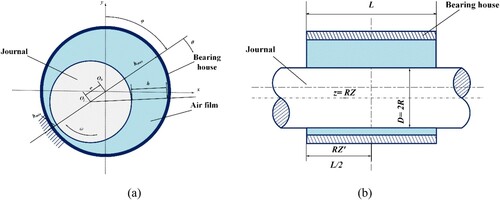
When the journal starts to rotate in a clockwise direction, the lubricating gas continuously accumulates in the convergent wedge and is compressed, leading to an increase of pressure in the convergent wedge. After the journal speed reaches a certain value, a lubricating air film is formed. The position of the journal is shifted to the left, as demonstrated in Figure , where the resultant pressure force generated by the lubricating air film is balanced by the load W.
Figure 2. Schematic diagram of axis balance position.
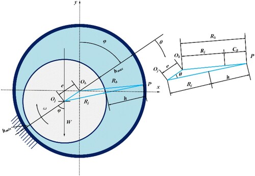
The equilibrium position of the axis Oj is described by the offset angle φ, which is defined as the angle between the line OjOb, and the eccentricity ratio ϵ, where ,
. The relevant geometric, operating and environmental parameters studied in the paper are summarized in Table .
Table 1. Geometric, operational and ambient bearing parameters.
2.1. Macroscopic numerical models and boundary conditions
2.1.1. Macroscopic numerical models
The lubrication state of the GLJB is the aerodynamic lubrication. The basic equation of the theoretical basis for it is the Navier–Stokes (N-S) equation, and the most obvious feature of the lubrication problem is that the fluid film thickness is much smaller than the geometric sizes of the other two dimensions, which makes it possible to simplify the N-S equation as follows:
(1)
(1)
As we all know, the equation of continuity is
(2)
(2)
Combining Equation (1) with Equation (2), the general form of the Reynolds equation, which is the basic equation of gas lubrication, can be derived:
(3)
(3) where h is the film thickness. Transferring the Reynolds equation from Cartesian coordinates into cylindrical coordinates with the relevant dimensionless parameters introduced, the Reynolds equation can be expressed as follows:
(4)
(4) where
(rad) is the angular coordinate:
Z is the dimensionless bearing length, P is the dimensionless pressure, H is the dimensionless film thickness, is the bearing number,
(Pa/s) is the dynamic viscosity,
(rpm) is the angular velocity of the bearing,
is the whirl frequency ratio,
is the dimensionless time and
(rad/s) is angular frequency of oscillation.
As can be seen from Figure , the angle is quite small in
so that
. Thereby, the air film thickness equation is obtained:
(5)
(5) As the gas-lubricated bearing works stably, the clearance is quite narrow (tens of microns or less) and appears to have different characteristics from under no-slip conditions. This effect is related to Kn, a measure of the deviation of the gas from a continuum medium, which is defined as follows:
(6)
(6) where h0 is the fluid’s characteristic size and
is the molecular free path, which is determined by the gas properties and state (Wang et al., Citation2016).
(7)
(7) where d is the diameter of molecular, n is the number density of molecules, p is the gas pressure, T is the gas temperature and k is Boltzmann’s constant.
2.1.2. Macroscopic boundary conditions
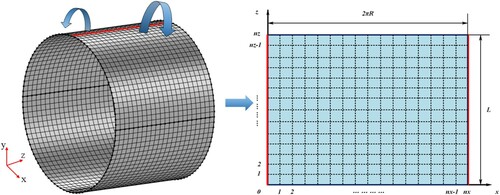
The finite difference method (FDM) is used in solving the Reynolds equation. The fluid domain is meshed as shown in Figure . The z- and x-directions are divided into equal parts, as nz and nx, respectively. Therefore, there are nz + 1 nodes along the length of the bearing in the z-direction, and nx + 1 nodes listed along the length of the circumference in the x-direction. The solution domain is defined as (0: nx, 0: nz).
Figure 3. Schematic diagram of mesh of macroscopic method.
The boundary conditions are defined as follows:
(8)
(8) In the circumferential direction, positions of x = 0 and x = nx coincide, so P(x, 0) = P(x, nz).
2.1.3. Macroscopic grids independence verification
Because the simulation results are affected by mesh generation modes, in order to verify the independence from macroscopic grid partitions, we gradually intensify the gridding of the model from 3 × 10³ to 1.9 × 10⁴ and the variation of maximum dimensionless pressure with the number of grids is shown in Figure , of which the relevant calculation parameters are shown in Table .
Figure 4. Macroscopic grids independence verification.
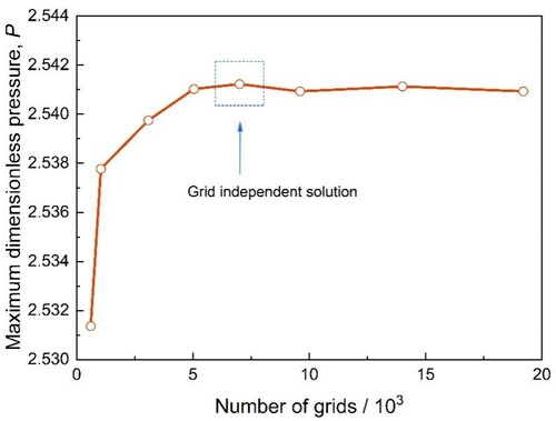
Table 2. Calculation parameters for macroscopic grids independence verification.
It can be seen that the pressure keeps basically constant after the number of grids exceeds 7 × 10³ and the mean deviation of the numerical result is around 0.9%. Comprehensively considering the computing time and precision factor, we choose this as the grid independent solution.
2.2. Mesoscopic numerical models and boundary conditions
2.2.1. Mesoscopic numerical models
Multi-relaxation-time LBM (MRT-LBM)
In the LBM, the two most used collision operators are the Bhatnagar–Gross–Ktook (BGK) (Qian & Orszag, Citation1993) and the MRT (Humières, Citation1994). Owing to the fact that the BGK collision operator has some disadvantages, such as that the viscosity depends on the physical results and the restriction of the density ratio (Zhang et al., Citation2018b), we choose the MRT in this simulation, of which the evolution equation is as follows (Lallemand & Luo, Citation2000):
(9)
(9) where
is the density distribution function for node x at time,
is the discrete velocity,
is the time step
, b is the total number of discrete velocities,
is the orthogonal transformation matrix and
is the equilibrium distribution function that relates the lubricant density
, velocity
and temperature
, which can be explained as follows:
(10)
(10) where e is the unit length lattice velocity,
,
is the lattice space step size,
is the time step,
is the lattice speed of sound,
(generally set as
for isothermal flow),
is the gas constant and
is the weight coefficient:
(11)
(11) In this research, we choose the two-dimensional nine-velocity (D2Q9) model, in which
is given by (Lallemand & Luo, Citation2000):
(12)
(12)
In Equation (9), the matrix M and diagonal matrix Λ are as follows (Lallemand & Luo, Citation2000; Li et al., Citation2018):
(13)
(13)
(14)
(14) where
defines the gas dynamic viscosity with
. Based on the simulation tests and the literature, the relaxation times in the diagonal matrix are chosen as
,
,
. The relaxation time
is determined by the shear viscosity.
The macroscopic variables, for instance lubricant density and velocity
, in dimensionless form are derived from the distribution function
and can be defined as
(15)
(15) The corresponding moment function is as follows:
(16)
(16)
The viscosity coefficient has a linear relationship with the
in Equation (6):
(17)
(17) where
. According to Equation (6),
can be obtained by
,
is given by
(
is the number of grids,
is the grid spacing), and
can be transformed into
(18)
(18)
Here, the relationship between and Kn can be acquired as (Guo et al., Citation2006):
(19)
(19) To associate the relaxation time with lubricant density
, we set
(20)
(20) Now, the LBM model suitable for continuous flow is set up, and the relationship between the Kn and the relaxation time
is put forward as well. The problem on disposing of the slip boundary will be expounded later.
Generalized form of interpolation supplemented LBM (GILBM)
In this section, it is our purpose to transform the MRT model governing equation (Equation 9) from uniform Cartesian coordinates into non-uniform curvilinear coordinates. That is, from the physical plane, expressed as , into computational planes, described as
. The process of solving the lattice Boltzmann equation (LBE) can be divided into two steps: collision and advection.
By substituting in Equation (9) with
, we can obtain the collision term described in generalized coordinates (Imamura et al., Citation2005) as
(21)
(21) After the transformation of the collision step, the advection term calculation is carried out and more discussion will be put forward. In Figure , the distributions of the vectors
on the physical and computational planes, respectively, are shown.
Figure 5. Discrete velocity vectors on the physical plane (a) and the computational plane (b).
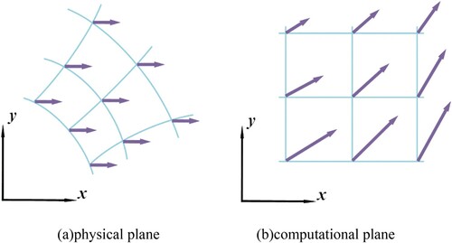
It is obvious that is kept the same in the physical plane, whereas it changes with variations of the grid nodes in the computational domain. Then, the contravariant velocities
are established:
(22)
(22) As a result, the advection term in Equation (9) is transformed into Equation (23):
(23)
(23) where
is the distance of particle advection and
is the time step.
(24)
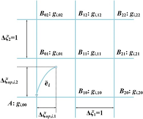
(24) In Equation (23), because the right-hand side is not always on the lattice nodes on the computational plane, the value cannot be exactly captured. Thus it is essential to introduce the interpolation method to ensure calculation accuracy. For the inner nodes, the second-order upwind interpolation method is applied. In contrast, for the boundary-adjacent nodes, on account of the limitation quantity of nodes, the second-order central difference interpolation method is adopted. The stencils used for the interpolation function are displayed in Figure , in which the
are the stencils depending on the positions of
(Imamura et al., Citation2005).
Figure 6. Stencils used for the interpolation function.
In order to keep the stability of numerical iteration, the time step ought to satisfy the Courante–Friedrichs–Lewy(CFL) condition (Imamura et al., Citation2005). Inspired by the traditional CFD methods, the calculation formula can be written as
(25)
(25) where
is the CFL number (
); herein,
. After that, during the advection, the particle will not exceed the domains of adjacent nodes and the stability of interpolation will be ensured.
2.2.2. Mesoscopic boundary conditions
Boundary conditions have a significant effect on the mesoscale LBM for the gas flow (Chen & Tian, Citation2009; Dongari et al., Citation2007; Myong, Citation2004; Wang et al., Citation2018). When dealing with the slip boundary of microflows, the Maxwell slip model (Dongari et al., Citation2007) is one of the most commonly seen types of model. Nevertheless, it has some disadvantages, of which the tangential momentum accommodation coefficient (TMAC) is difficult to evaluate, for it depends on the fluid types, surface material properties and geometry shapes. Here, we decide to adopt the Langmuir slip model (Myong, Citation2004). Without taking the surface diffusion effect into consideration, for the first-order slip velocity can be written as
(26)
(26) where
is the first-order slip coefficient,
is the local velocity adjacent to the wall and
is the local velocity at the wall. Combining Equation (25) with the Maxwell first-order slip model,
can be derived as
(27)
(27) where
is the first adjustment coefficient and
is the grid number.
As previously mentioned, the first-order slip model for the slip flow regime is set up. However, the accuracy of the first-order slip model does not satisfy the transition regime. We choose to introduce the second-order slip velocity by the Langmuir model (Wang et al., Citation2018):
(28)
(28) where
is the second-order slip coefficient and
is the local velocity adjacent to node
. Similarly to the procedure of Equation (27), we can derive the
as follows:
(29)
(29) where
is the second adjustment coefficient.
According to the non-equilibrium extrapolation (NEE) scheme (Chen & Tian, Citation2009), the distribution function can be divided into two sections, the equilibrium and the non-equilibrium sections:
(30)
(30) We can transform the Langmuir slip model into the NEE scheme. The first-order slip boundary and the second-order slip boundary can be expressed as Equations (31) and (32). Then, we have the slip boundary conditions for the slip flow and the transition flow regimes:
(31)
(31)
(32)
(32)
2.2.3. Mesoscopic grids independence verification
Owing to the fact that the method of mesh generation has a great influence on the simulation results, we need to verify the independence of mesoscopic grid partition. The bearing clearance is meshed as shown in Figure . As we gradually intensify the grids from 1.38 × 10⁵ to 2.2 × 10⁶, the variation of maximum dimensionless pressure with the number of grids is shown in Figure , of which the relevant calculation parameters are shown in Table .
Figure 7. Schematic diagram of mesh of mesoscopic method.
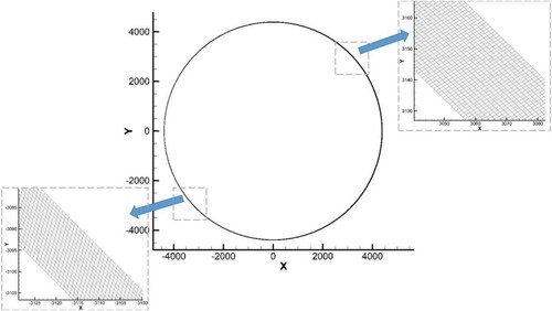
Table 3. Calculation parameters for mesoscopic grids independence verification.
Figure 8. Mesoscopic grids independence verification.
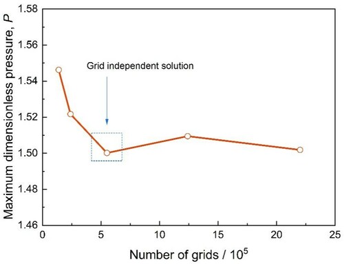
It can be seen that the pressure keeps basically constant after the number of grids exceeds 5.5 × 10⁵ and the mean deviation of the numerical result is less than 0.9%. Comprehensively considering the computing time and precision factor, we choose this as the grid independent solution.
3. Model validation
3.1. Macroscopic model validation
The curves are shown in Figure of the lubricant air film pressure and film thickness distributions calculated by the macroscopic method compared with those in the literature (Peng & Khonsari, Citation2006; Xu, Citation2012), the data of which are highly consistent with the existing experimental results (Strom, Citation1988). The relative comparison case parameters are shown in Table . The maximum error values occur at the maximum pressure and thickness peaks, which are less than 3%. It can be concluded that the macroscopic method is valid and has high numerical accuracy.
Figure 9. Comparison of macroscopic method simulation results and experimental data in the literature: (a) dimensionless pressure distribution with angular coordinate; (b) dimensionless film thickness distribution with angular coordinate.
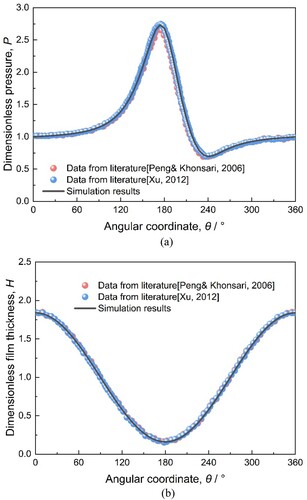
Table 4. Parameters of comparison examples in the literature (Peng & Khonsari, Citation2006; Xu, Citation2012).
3.2. Mesoscopic model validation
The radial velocity profile results of the microcylindrical Couette flow are displayed in Figure compared with those obtained by the mesoscopic LBM and analytic method in the literature (Sun et al., Citation2005), respectively. The mesh division of LBM is shown in Figure .
Figure 10. Comparison of mesoscopic method simulation results and analytical results.
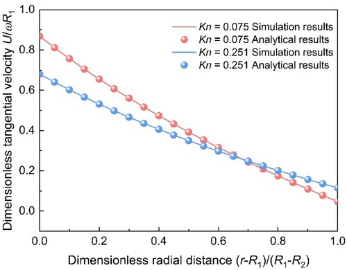
Figure 11. Grids of the microcylindrical Couette flow.
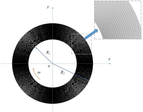
The inner journal with radius R1 rotates clockwise with angular velocity and the outer cylinder house with radius R2 keeps stationary, where R1 : R2 = 3 : 5. The analytic model in the literature (Sun et al., Citation2005) is a combination of the N-S equation and the Maxwell’s diffusion model, expressed as follows:
(33)
(33) where
(34)
(34)
Then, Equation (33) can be rewritten as
(35)
(35) where
is the tangential velocity,
and
are the tangential momentum accommodation coefficients (TMACs) of the inner and outer cylindrical surfaces (set separately as one) and
is the radial parameter in the cylindrical-polar coordinate
reference frame. The error value of the maximum pressure is less than 3%, which indicates that the introduced mesoscopic LBM obtains reasonable feasibility and accuracy.
4. Results and discussion
4.1. Air film pressure, thickness, velocity distribution and the backflow phenomenon under different eccentricity ratios
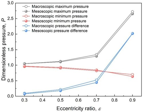
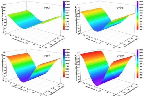
It is shown in Figure that when the eccentricity ratios vary from ϵ = 0.3 to ϵ = 0.9, with ω = 5 × 10⁴ rpm, the maximum and minimum lubricating air film pressure peaks will increase and decrease, respectively. Simultaneously, the pressure differences between the two peaks increase as the eccentricity ratios increase. It can be seen from Figure that the variation trends of the maximum, minimum and pressure difference are stable before ϵ = 0.5, the slopes incline more obviously from ϵ = 0.5 to ϵ = 0.7, and the inclinations change rapidly after ϵ = 0.7. Additionally, the tendency of curves simulated by both methods are similar. Nevertheless, some differences exist: first, the width of the peaks simulated by LBM is narrower than that of the Reynolds equation (shown in Figure ), which represents the fact that the area of the high pressure zone simulated by the former is less than that of the latter; also, the pressure variation is more concentrated. The peaks simulated by LBM appear slightly earlier than those of the Reynolds equation. Third, the minimum pressure peak obtained by LBM is distinctly lower than that of the Reynolds equation at ϵ = 0.9 (shown in Figure ); however, the pressure differences of the maximum/minimum peaks of results from both methods are close. The errors in the maximum pressure by the two methods are 0.4%, 1.3%, 3.9%, 2.5% at ϵ = 0.3, ϵ = 0.5, ϵ = 0.7 and ϵ = 0.9, respectively. Meanwhile, those in the minimum pressure are 1.4%, 2.5%, 3.1%, 9% at ϵ = 0.3, ϵ = 0.5, ϵ = 0.7 and ϵ = 0.9, respectively.
Figure 12. Air film pressure distributions under different eccentricity ratios.
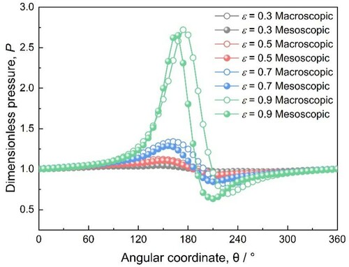
Figure 13. Variations of pressure under different eccentricity ratios.
These distinctions could be caused by, first, the transformation of the wedge-shape gas flow channel will be intensified by increasing the eccentricity ratio. The shearing force of the flow near the journal surface around the pressure peaks will change more extensively, the friction and viscous dissipation may increase more severely leading to the reduction of the pressure peak areas. Secondly, the gas bearing has a certain negative pressure zone with pressure lower than the ambient pressure, mainly around the minimum pressure peak position of the bearing, where lubricating gas can be sucked in to supply lubricant for bearing. With the increase of tbe eccentricity ratio, not enough lubrication air is sucked into the clearance in the negative pressure zone to fill up the loss caused by the high pressure output, resulting in a decrease of the minimum pressure peak. Thirdly, the slip boundary accelerates the decrease of the maximum air film pressure, making the maximum pressure peak overall narrower than that of the macroscopic result. Additionally, the continuum assumption could be the reason for a higher maximum air film pressure in the macroscopic methods, which is mentioned by Zhang et al. (Citation2016).
To better understand the influence of eccentricity ratios on the bearing lubricant flow characteristics, the air flow streamlines in the maximum clearance are simulated by the mesoscopic LBM, which is correspondingly displayed in Figure . On account of the shear stress driving function on the lubricant air film caused by the rotating journal shaft, the velocity of the air film close to the journal surface is higher than that adjacent to the bearing house inner surface. With an increase in the eccentricity ratio, the area of the relative low velocity domain expands; in contrast, the area of the relatively high velocity domain shrinks. Then, at the eccentricity ratio ϵ = 0.3, the streamlines in the clearance are evenly distributed in the same direction. At ϵ = 0.5, vorticity streamlines appear around the bearing house inner surface, indicating backflow occurring on the side close to the bearing sleeve. As it reaches ϵ = 0.7, with the space of maximum clearance becoming larger, and the relative low-velocity air flow increasing, collisions between the relatively high-velocity and low-velocity air flows are aggravated, leading to the air congestion phenomenon in the wedge-shape channel becoming more severe and the vortices appearing more obviously. When the eccentricity ratio reaches ϵ = 0.9, both the vorticity streamlines become more intense and the area of the vortex becomes even larger, and a more intensified backflow phenomenon occurs. This can also explain the drop of the minimum pressure peak. Furthermore, we can explore the reasons for the form of Figure further by means of Figure .
Figure 14. Change of air film backflow under different eccentricity ratios.
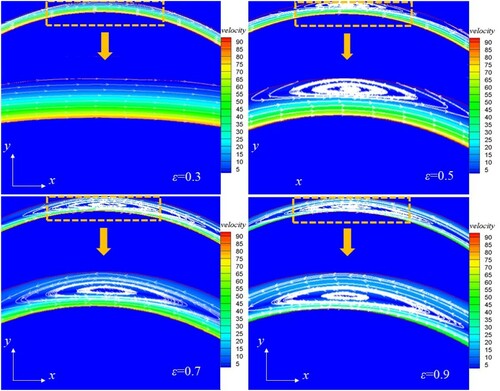
Figure 15. Flow velocity distribution under different eccentricity ratios.
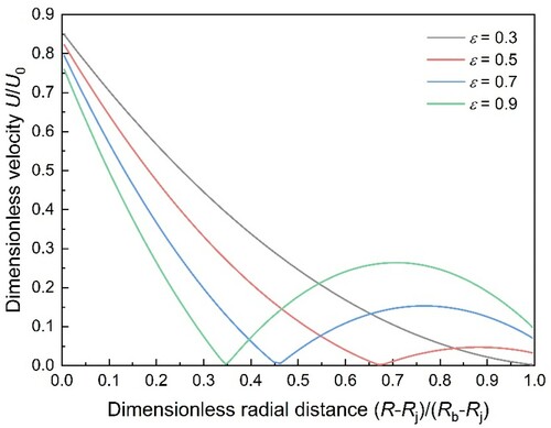
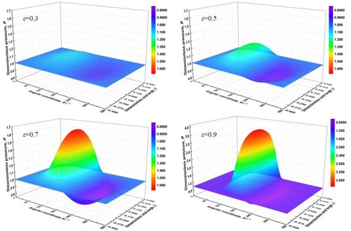
Figure 16. Three-dimensional pictures of air film pressure distribution under different eccentricity ratios.
As shown in Figure , the dimensionless velocity varies with the dimensionless radial distance under different eccentricity ratios. At the low eccentricity ratio ϵ = 0.3, with the dimensionless radial distance shifting from the journal to the bearing house, the velocity of lubricant air flow declines approximately linearly, which is similar to the velocity distribution of a typical traditional Couette flow. When it reaches ϵ = 0.5, the air flow velocity at first goes down then lifts again around a relative position of 0.68, indicating that an inverse flow occurs. When it goes from ϵ = 0.7 to ϵ = 0.9, the reversal trends of the velocity flow appear more obvious, with the velocity difference turning larger. Because, the larger the eccentricity ratio is, the higher the maximum air film thickness will be, combined with the greater effect of the inverse pressure gradient, the shear force becomes insufficient, and more violent backflow occurs. Furthermore, the squeeze function of the increasing relatively-low velocity air flow to that of the decreasing relatively-high velocity air flow strengthens the phenomenon, which could be one of the primary causes of the friction loss in bearing operation reported by Serrano et al. (Citation2020).
Displayed in Figures and are the corresponding three-dimensional cloud pictures of air film pressure and thickness distributions changing under different eccentricity ratios, from ϵ = 0.3 to ϵ = 0.9 with ω = 5 × 10⁴ rpm, by the macroscopic method. It can be seen that, as the angular coordinate θ gradually increases from 0° to 360°, the air film pressure distribution exhibits an increase–decrease–increase trend. In contrast, the air film thickness distribution presents a decrease–increase trend. With the eccentricity ratios increasing from ϵ = 0.3 to ϵ = 0.9, the maximum air film pressure peaks elevate and the minimum air film pressure peaks reduce. While the minimum air film pressure peaks reduce, the maximum air film pressure peaks elevate. Those appearances could be caused for the following reasons. First, for the eccentricity ratio representing the bearing load, the higher the eccentricity ratio is, the heavier the load on the journal will be, and the stronger the squeezing action on the lubricant air film will be. On account of the compressibility of gas, the minimum thickness of the air film shrinks, leading to an intensified cross-section effect variation. As a consequence, the maximum pressure peak is enhanced near the maximum air film pressure peak. Secondly, at high eccentricity ratios, there will be much more space near the maximum air film thickness position, which makes the minimum air film pressure peak reduce. The difference in pressure between the high-pressure and low-pressure zones expands, leading to more pressure gap existing between the pressure peaks. Moreover, the sharp jump in the maximum air film pressure peak at ϵ = 0.9 is caused by the severe compression of the air film in the clearance, and the interval is too narrow to flow through, causing the air pressure to increase abruptly, which is in agreement with the results reported in the literature (Shalash & Schiffmann, Citation2020). The study indicates that, by keeping the eccentricity ratio at an appropriately high level, the working performance of the GLJB will be improved.
Figure 17. Three-dimensional pictures of air film thickness distribution under different eccentricity ratios.
4.2. Air film pressure, velocity distribution under different bearing speeds
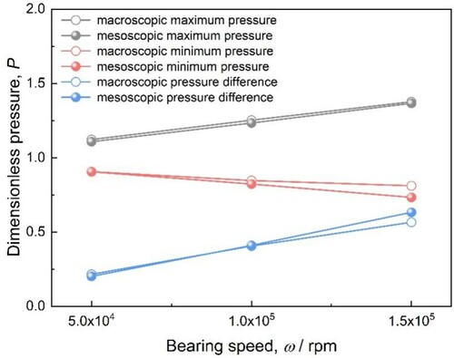
The change of the air film pressure distribution withdifferent bearing speeds is shown in Figure , which is simulated by both the macroscopic and mesoscopic methods at bearing speeds ranging from ω = 5 × 10⁴ rpm to ω = 1.5 × 10⁵ rpm and ϵ = 0.5. With increasing bearing speed, the peaks of the maximum and the minimum air film pressure will increase and decrease, respectively. The pressure difference between the two peaks of the air clearance enlarges, as displayed in Figure . By comparison, the pressure distribution obtained by the two methods are generally consistent with each other. However, the errors of the results change with the speeds—the errors in the maximum pressure are 1.3%, 1.2% and 0.81% at ω = 5 × 10⁴ rpm, ω = 1 × 10⁵ rpm and ω = 1.5 × 10⁵ rpm, respectively. Meanwhile, those in the minimum pressure are 0.08%, 2.8% and 9.6%, respectively.
Figure 18. Air film pressure distribution under different bearing speeds.
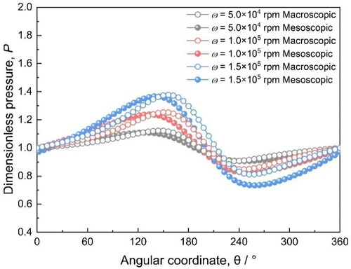
Figure 19. Variations of pressure under different bearing speeds.
We need to explore the reasons explaining this phenomenon. As shown in Figure , with the enhancement of journal speeds, the velocity of gas flow is accelerated and the radial gradient of the lubricating film airflow velocity is increased, thereby giving rise to a growth in the tangential shear force, and causing an increase in the viscous friction force. To some extent, the higher the speed, the greater the radial gradient of the lubricating film air flow velocity will be, and the larger the tangential shear force that will form. As a result of the shear force function, the gas flow velocity difference in the boundary layer near the journal surface is enlarged. As is shown in Figure , the bearing capacity of the GLJB will be enhanced. It can be concluded that an increase of bearing speed within a certain range is beneficial for the GLJB to undertake a higher bearing load at relative lower eccentricity ratio and larger attitude angle. However, it is worth noting that the bearing speed is not simply ‘the higher the better’. When the bearing speed is high enough, the slip function of lubrication flow near the journal surface is strengthened, and gas congestion can form around the pressure peaks, as mentioned in the literature (Zhang et al., Citation2016). Excessive bearing speed can lead to amounts of friction loss that will negatively influence the operating stability and working life of the GLJB. As a consequence, the working performance of the GLJB will not always be improved with a rise in the bearing speed.
Figure 20. Flow velocity distribution under different bearing speeds.
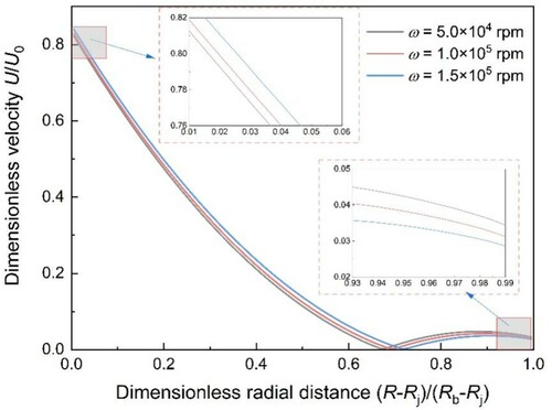
Figure 21. Variation of eccentricity ratio with bearing loads under different bearing speeds.
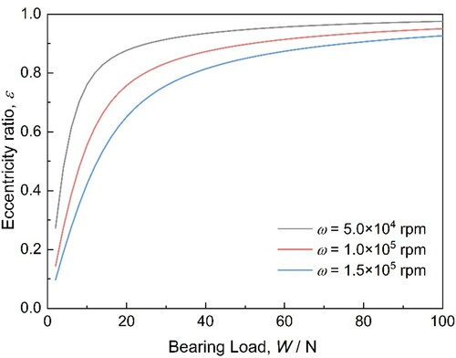
Figure 22. Variation of attitude angle with bearing loads under different bearing speeds.
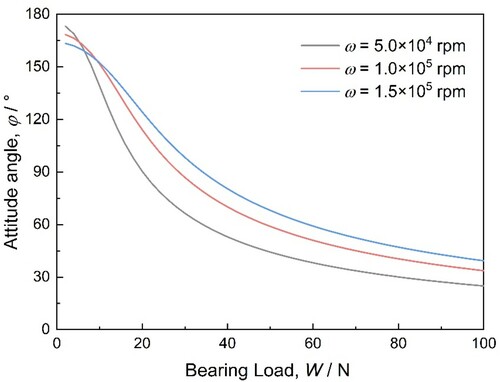
Figure illustrates the relationship between the eccentricity ratio and the bearing load at different bearing speeds. When the bearing load rises, the eccentricity ratios will first lift rapidly to a relative high level, then the increase in the slopes of the eccentricity ratio become gentle and linear. It is because, at the beginning of the loading effect, the air flow will be greatly compressed to small volumes, resulting the rapid growth of the eccentricity ratio. After that, due to the limited compressibility of air and the clearance space, gas compression becomes difficult and the distance between the journal and the bearing quite narrow, then the growth of the eccentricity ratio is slight. Moreover, to tolerate the same load on the bearing, a higher speed rotating bearing needs a lower eccentricity ratio than that of lower speed rotating bearing, which is a function of kinetic energy, which can counteract the effect of bearing load.
As shown in Figure , the attitude angle changes with the variation in bearing load at different bearing speeds. It can be observed that the larger the bearing speed, the less obvious the variation of the attitude angle will be. When the bearing load is higher than 40 N, all the attitude angels are less than 90°, which indicates that the effect of the difference in bearing load on the attitude angle is shrinking. According to fluid lubrication theory, the smaller the attitude angle, the more stable the bearing will be, and the less the vertical component of the force on the lubricant film will be, which is usually through the centrelines. Thus, to some extent, with an increase in bearing speed, the stability of the journal bearing will become better.
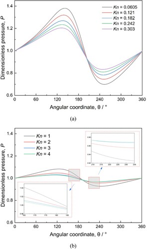
Figure 23. Air film pressure distribution under different values of Kn.
4.3. Air film pressure distribution under different Kn
Variations in the lubricating air film pressure distributions with Kn obtained by the LBM are displayed in Figure . As an important parameter to characterize channel size and fluid characteristics, Kn can be used to classify the gas flow situations into different flow regimes (Sun et al., Citation2018). Within the tiny journal-bearing house clearance, the Kn of lubricating gas flow could rise to a high value. Owing to the continuum assumption, the conventional macroscopic method is not available at high Kn conditions, and the advantage of the mesoscopic method is demonstrated. In this research, Kn varies from 0.0605 to 0.303 in Figure (a) and from 1 to 4 in Figure (b), involving the slip flow and the transition flow regimes, with the aim of exploring the effect of Kn on the bearing pressure distribution. It is shown in Figure that, as Kn increases, the maximum and minimum pressure peaks will decline and rise, and the pressure gap between the two peaks will diminish. Additionally, the variation speed of the maximum pressure peaks will change from high to low with the enhancement of Kn. Comparing Figures (a) and (b), it can be seen that, at relative large Kn, the pressure transformation is different from that at relatively low Kn, although both of them belong to the transition regime. That is, if Kn is high enough, the influence of Kn on the pressure will be limited. This phenomenon could be caused by the increased Kn leading to a more pronounced rarefaction effect, making the wall slip effect of the bearing to strengthen, and the bearing's shear force on the gas to be decreased, resulting in decreased maximum pressure peaks. Moreover, if Kn is too high, the residual space for the rarefaction effect on the lubricant pressure will be too narrow, which will give rise to a very small difference in pressure peaks. To sum up, Kn will have an effect on the pressure distributions; however, in the tiny clearance of a GLJB, the degree of influence of the rarefaction effect on the pressure distribution will reduce with an increase in Kn. Furthermore, it indicates that the LBM can be introduced as an ideal method for research in high Kn conditions, which is of inherent compatibility with the slip boundary.
5. Conclusion
In this research, we propose a multiscale numerical investigation method combining the macroscopic Reynolds equation and the mesoscopic LBM to simulate the air film flow in the narrow clearance of a GLJB. At different bearing speeds, eccentricity ratios and slip conditions (Kn), the changing rules of the air film pressure, thickness and velocity distributions are investigated. The differences between the results of the two methods are compared and analysed. In addition, an interesting backflow phenomenon in the clearance is observed by the LBM and the reason for its formation is discussed. To sum up, conclusions are given as follows.
For the Reynold equation and the LBM, the former has a clear physical meaning and can be used as a proof for the latter in the simulation of GLJBs. In contrast, the latter can be applied to capture the velocity distributions and backflow phenomenon at the multiscale level as a complement to the former.
The multiscale model can be adopted to simulate the air flow of a GLJB at high Kn conditions in both the slip or transition flow regimes, which overcomes the disadvantage of the continuum hypothesis. The LBM can be an ideal method for research on the rarefaction effect.
When the eccentricity ratios increase from ϵ = 0.3 to ϵ = 0.9, the errors in the maximum pressure peaks by the two methods are 0.4%, 1.3%, 3.9% and 2.5%, respectively. In contrast, those in the minimum pressure peaks are 1.4%, 2.5%, 3.1% and 9%, respectively. When bearing speeds accelerate from ω = 5 × 10⁴ rpm to ω = 1.5 × 10⁵ rpm, the errors in the maximum pressure peaks are 1.3%, 1.2%, 0.81%, respectively. In contrast, those in the minimum pressure peaks are 0.08%, 2.8%, 9.6%, respectively.
This study indicates that, by keeping the eccentricity ratio and bearing speed at appropriately high levels, the working performance of GLJBs will be improved. However, the performance will not always be promoted with a rise in bearing speed. When Kn enhances, the maximum and minimum pressure peaks will decrease and increase, respectively; however, the extent of influence of the rarefaction effect on the pressure distribution will reduce after Kn exceeds a certain degree.
Nomenclature
Symbols
| C | = | Radial clearance (m) |
| Co | = | Radial average clearance (m) |
| c | = | Lattice velocity |
| cs | = | Lattice speed of sound |
| = | Molecular average motion speed | |
| D | = | Diameter of journal (m) |
| d | = | Effective molecular diameter (m) |
| e | = | Eccentricity |
| ei | = | Discrete velocity |
| Fi | = | External forcing term |
| = | Particle density distribution function | |
| H | = | Dimensionless film thickness |
| h | = | Film thickness, gap height (m) |
| h0 | = | Fluid characteristic size (m) |
| Kn | = | Knudsen number |
| k | = | Boltzmann's constant, 1.38 × 10⁻²³ (J/K) |
| L | = | Bearing length (m) |
| M | = | Orthogonal transformation matrix |
| M−1 | = | Inverse orthogonal transformation matrix |
| NH | = | Number of lattices |
| n | = | Number density of gas molecules |
| P | = | Dimensionless pressure |
| pa | = | Ambient pressure (Pa) |
| p | = | Pressure of the gas (Pa) |
| R | = | Radial pressure in the cylindrical-polar coordinate (m) |
| Rb | = | Radius of bearing (m) |
| Rj | = | Radius of journal (m) |
| S | = | Diagonal relaxation matrix |
| T | = | Temperature of the gas (K) |
| t | = | time (s) |
| = | Dimensionless time | |
| U | = | Tangential velocity of bearing (m/s) |
| u | = | Velocity vector |
| uf | = | Local velocity adjacent to the wall |
| uslip | = | Slip velocity |
| uw | = | Local velocity at wall |
| W | = | Bearing load (N) |
| x | = | Circumference direction |
| y | = | Radial direction |
| Z | = | Dimensionless bearing length |
| z | = | Axial direction |
Greek
| = | whirl frequency ratio | |
| Δx | = | Grid spacing |
| δt | = | Time step |
| ϵ | = | Eccentricity ratio |
| κ1, κ2 | = | Slip coefficients |
| λ | = | Molecular free path (m)/CFL number |
| μ | = | Dynamic viscosity (Pa/s) |
| θ | = | Angular coordinate (rad) |
| Λ | = | Diagonal matrix |
| Λ | = | Bearing number |
| τ | = | Relaxation time that relies on the fluid kinematic viscosity |
| τs | = | Relaxation time |
| τv | = | Gas dynamic viscosity |
| ξ, η | = | Coordinates on the computational plane |
| φ | = | Attitude angle (rad) |
| ω | = | Bearing speed (rpm) |
| ωi | = | Weight coefficient |
| = | Angular frequency of oscillation |
Superscripts
| * | = | Probability |
| eq | = | Equilibrium |
| 1 | = | First-order |
| 2 | = | Second-order |
Subscripts
| b | = | Bearing |
| j | = | Journal |
| i | = | Interacting atoms or component |
| o | = | Original/preload |
| s | = | Sound |
Disclosure statement
No potential conflict of interest was reported by the authors.
Additional information
Funding
References
- Andrés, L. S., & Rodríguez, B. (2020). Experiments with a rotor-hybrid gas bearing system undergoing maneuver loads from its base support. Journal of Engineering for Gas Turbines and Power, 142(11), 111004. https://doi.org/https://doi.org/10.1115/1.4048651
- Arghir, M., & Benchekroun, O. (2019). A simplified structural model of bump-type foil bearings based on contact mechanics including gaps and friction. Tribology International, 134, 129–144. https://doi.org/https://doi.org/10.1016/j.triboint.2019.01.038
- Baum, C., Hetzler, H., & Schroders, S. (2021). A computationally efficient nonlinear foil air bearing model for fully coupled, transient rotor dynamic investigations. Tribology International, 153, 106434. https://doi.org/https://doi.org/10.1016/j.triboint.2020.106434
- Bryant, M. D. (2013). Reynolds equation for compressible fluid or gas film. In Q. J. Wang, & Y. W. Chung (Eds.), Encyclopedia of tribology (pp. 2773–2775). Springer.
- Chen, G. D., Ju, B. F., & Fang, H. (2019). Air bearing: Academic insights and trend analysis. The International Journal of Advanced Manufacturing Technology, 106(3-4), 1191–1202. https://doi.org/https://doi.org/10.1007/s00170-019-04663-5
- Chen, S., & Tian, Z. (2009). Simulation of microchannel flow using the lattice Boltzmann method. Physica A: Statistical Mechanics and its Applications, 388(23), 4803–4810. https://doi.org/https://doi.org/10.1016/j.physa.2009.08.015
- Chen, S. G., Zhang, C. H., & Feng, Y. T. (2016). Three-dimensional simulations of Bingham plastic flows with the multiple-relaxation-time lattice Boltzmann model. Engineering Applications of Computational Fluid Mechanics, 10(1), 346–358. https://doi.org/https://doi.org/10.1080/19942060.2016.1169946
- Dongari, N., Agrawal, A., & Agrawal, A. (2007). Analytical solution of gaseous slip flow in long microchannels. International Journal of Heat and Mass Transfer, 50(17-18), 3411–3421. https://doi.org/https://doi.org/10.1016/j.ijheatmasstransfer.2007.01.048
- Ghalandari, M., Koohshahi, E. M., & Mohamadian, F. (2019). Numerical simulation of nanofluid flow inside a root canal. Engineering Applications of Computational Fluid Mechanics, 13(1), 254–264. https://doi.org/https://doi.org/10.1080/19942060.2019.1578696
- Gokaltun, S., & Dulikravich, G. S. (2007, June 18–20). Lattice Boltzmann method for steady gas flows in microchannels with imposed slip wall boundary condition [Paper presentation]. Proceedings of the ASME 5th International Conference on Nanochannels, Microchannels and Minichannels, Puebla, Mexico.
- Gu, L. L., Guenat, E., & Schiffmann, J. (2020a). A Review of grooved dynamic Gas bearings. Applied Mechanics Reviews, 72(1), 010802. https://doi.org/https://doi.org/10.1115/1.4044191
- Gu, Y. P., Ren, G. X., & Zhou, M. (2020b). A fully coupled elastohydrodynamic model for static performance analysis of gas foil bearings. Tribology International, 147, 394–400. https://doi.org/https://doi.org/10.1016/j.triboint.2020.106297.
- Guiet, J., Reggio, M., & Teyssedou, A. (2011). Implementation and application of the Lattice Boltzmann method using matlab. Engineering Applications of Computational Fluid Mechanics, 5(1), 117–126. https://doi.org/https://doi.org/10.1080/19942-060.2011.11015356
- Guo, Z., Zhao, T. S., & Shi, Y. (2006). Physical symmetry, spatial accuracy, and relaxation time of the lattice Boltzmann equation for microgas flows. Journal of Applied Physics, 99(7), 074903. https://doi.org/https://doi.org/10.1063/1.2185839
- Guo, Z. Y., Cao, Y. L., & Feng, K. (2019). Effects of static and imbalance loads on nonlinear response of rigid rotor supported on gas foil bearings. Mechanical Systems and Signal Processing, 133, 106271. https://doi.org/https://doi.org/10.1016/j.ymssp.2019.106271
- Guo, Z. Y., Peng, L., & Feng, K. (2017). Measurement and prediction of nonlinear dynamics of a gas foil bearing supported rigid rotor system. Measurement, 121, 205–217. https://doi.org/https://doi.org/10.1016/j.measurement.2017.12.039
- Heshmat, C. A., Xu, D. S., & Heshmat, H. (2000). Analysis of gas lubricated foil thrust bearings using coupled finite element and finite difference methods. Journal of Tribology, 122(1), 199–204. https://doi.org/https://doi.org/10.1115/1.555343
- Heshmat, H., Walowit, J. A., & Pinkus, O. (1983). Analysis of gas-lubricated foil journal bearings. Journal of Lubrication Technology, 105(4), 647–655. https://doi.org/https://doi.org/10.1115/1.3254697
- Humières, D. (1994). Generalized lattice-Boltzmann equations. In D. P. Weaver, & B. D. Shizgal (Eds.), AIAA rarefied gas dynamics: Theory and applications (pp. 450–458). American Institute of Aeronautics and Astronautics Inc. https://doi.org/https://doi.org/10.2514/5.9781600866319.0450.0458.
- Imamura, T., Suzuki, K., & Nakamura, T. (2005). Acceleration of steady-state lattice Boltzmann simulations on non-uniform mesh using local time step method. Journal of Computational Physics, 202(2), 645–663. https://doi.org/https://doi.org/10.1016/j.jcp.2004.08.001
- Jiao, C., Leng, Z., & Zou, D. (2021). Numerical research of the infinitely wide wedge flow based on the lattice Boltzmann method. Proceedings of the Institution of Mechanical Engineers, Part J: Journal of Engineering Tribology, 235(2), 343–350. https://doi.org/https://doi.org/10.1177/1350650120962929
- Lai, T. W., Guo, Y., & Zhao, Q. (2018). Numerical and experimental studies on stability of cryogenic turbo-expander with protuberant foil gas bearings. Cryogenics, 96, 62–74. https://doi.org/https://doi.org/10.1016/j.cryogenics.2018.10.009
- Lallemand, P., & Luo, L. S. (2000). Theory of the lattice Boltzmann method: Dispersion, dissipation, isotropy, Galilean invariance, and stability. Physical Review E, 61(6), 6546–6562. https://doi.org/https://doi.org/10.1103/PhysRevE.61.6546
- Larsen, J. S., Santos, I. F., & Osmanski, S. V. (2016). Stability of rigid rotors supported by air foil bearings: Comparison of two fundamental approaches. Journal of Sound and Vibration, 381, 179–191. https://doi.org/https://doi.org/10.1016/j.jsv.2016.06.022
- Lehn, A., Mahner, M., & Schweizer, B. (2017). A contribution to the thermal modeling of bump type air foil bearings: Analysis of the thermal resistance of bump foils. Journal of Tribology, 139(6), 061702. https://doi.org/https://doi.org/10.1115/1.4036631
- Li, Q., Yu, Y., & Zhou, P. (2018). Enhancement of boiling heat transfer using hydrophilic-hydrophobic mixed surfaces: A lattice Boltzmann study. Applied Thermal Engineering, 132, 490–499. https://doi.org/https://doi.org/10.1016/j.applthermaleng.2017.12.105
- Li, Y. Y., Lei, G., & Sun, Y. (2017). Effect of environmental pressure enhanced by a booster on the load capacity of the aerodynamic gas bearing of a turbo expander. Tribology International, 105, 77–84. https://doi.org/https://doi.org/10.1016/j.triboint.2016.09.027
- Liu, Z. X., Fang, Y., & Song, A. P. (2016). A multi-domain decomposition strategy for the lattice Boltzmann method for steady-state flows. Engineering Applications of Computational Fluid Mechanics, 10(1), 72–85. https://doi.org/https://doi.org/10.1080/19942060.2015.1092743
- Myong, R. S. (2004). A generalized hydrodynamic computational model for rarefied and microscale diatomic gas flows. Journal of Computational Physics, 195(2), 655–676. https://doi.org/https://doi.org/10.1016/j.jcp.2003.10.015
- Nie, X. B., Doolen, G. D., & Chen, S. Y. (2002). Lattice-Boltzmann simulations of fluid flows in MEMS. Journal of Statistical Physics, 107(1/2), 279–289. https://doi.org/https://doi.org/10.1023/A:1014523007427
- Nielsen, B. B., & Santos, I. F. (2017). Transient and steady state behaviour of elasto–aerodynamic air foil bearings, considering bump foil compliance and top foil inertia and flexibility: A numerical investigation. Proceedings of the Institution of Mechanical Engineers, Part J: Journal of Engineering Tribology, 231(10), 1235–1253. https://doi.org/https://doi.org/10.1177/13506501-17689985
- Peng, Z.-C., & Khonsari, M. M. (2006). A thermohydrodynamic analysis of foil journal bearings. Journal of Tribology, 128(7), 534–541. https://doi.org/https://doi.org/10.1115/1.2197526
- Qian, Y. H., & Orszag, S. A. (1993). Lattice BGK models for the Navier–Stokes equation: Nonlinear deviation in compressible regimes. Europhysics Letters (EPL), 21(3), 255–259. https://doi.org/https://doi.org/10.1209/0295-5075/21/3/001
- Rao, T. V. V. L. N. (2009). Theoretical prediction of journal bearing stability characteristics based on the extent of the slip region on the bearing surface. Tribology Transactions, 52(6), 750–758. https://doi.org/https://doi.org/10.1080/10402000903097387
- Rom, M., & Müller, S. (2019). A new model for textured surface lubrication based on a modified Reynolds equation including inertia effects. Tribology International, 133, 55–66. https://doi.org/https://doi.org/10.1016/j.triboint.2018.12.030
- Salih, S. Q., Aldlemy, M. S., & Rasani, M. R. (2019). Thin and sharp edges bodies-fluid interaction simulation using cut-cell immersed boundary method. Engineering Applications of Computational Fluid Mechanics, 13(1), 860–877. https://doi.org/https://doi.org/10.1080/19942060.2019.1652209
- Samanta, P., Murmu, N. C., & Khonsari, M. M. (2019). The evolution of foil bearing technology. Tribology International, 135, 305–323. https://doi.org/https://doi.org/10.1016/j.triboint.2019.03.021
- Sergi, D., Grossi, L., & Leidi, T. (2015). Lattice Boltzmann simulations on the role of channel structure for reactive capillary infiltration. Engineering Applications of Computational Fluid Mechanics, 9(1), 301–323. https://doi.org/https://doi.org/10.1080/19942-060.2015.1026432
- Serrano, J. R., Olmeda, P., & Arnau, F. J. (2020). A holistic methodology to correct heat transfer and bearing friction losses from hot turbocharger maps in order to obtain adiabatic efficiency of the turbomachinery. International Journal of Engine Research, 21(8), 1314–1335. https://doi.org/https://doi.org/10.1177/1468087419834194
- Shalash, K., & Schiffmann, J. (2020). An instrumented high-speed rotor with embedded telemetry for the continuous spatial pressure profile measurement in gas lubricated bearings: A proof of concept. Journal of Engineering for Gas Turbines and Power, 142(4), 041006. https://doi.org/https://doi.org/10.1115/1.4044797
- Sim, K., Lee, Y. B., & Kim, T. H. (2013). Effects of mechanical preload and bearing clearance on rotordynamic performance of lobed gas foil bearings for oil-free turbochargers. Tribology Transactions, 56(2), 224–235. https://doi.org/https://doi.org/10.1080/10402004.2012.737502
- Strom, T. (1988). Advanced gas turbine (AGT) technology development project: final report. (Report No. CR-180891). NASA, United States. https://www.osti.gov/biblio/5004110.
- Sun, Y. H., Barber, R. W., & Emerson, D. R. (2005). Inverted velocity profiles in rarefied cylindrical Couette gas flow and the impact of the accommodation coefficient. Physics of Fluids, 17(4), 047102. https://doi.org/https://doi.org/10.1063/1.1868034
- Sun, Z., Shi, J. T., & Wu, K. L. (2018). Transport capacity of gas confined in nanoporous ultra-tight gas reservoirs with real gas effect and water storage mechanisms coupling. International Journal of Heat and Mass Transfer, 126, 1007–1018. https://doi.org/https://doi.org/10.1016/j.ijheatmasstransfer.2018.05.078
- Wang, L., Xu, Z., & Guo, Z. L. (2016). Lattice Boltzmann simulation of separation phenomenon in a binary gaseous flow through a microchannel. Journal of Applied Physics, 120(13), 134306. https://doi.org/https://doi.org/10.1063/1.4964249
- Wang, L., Zeng, Z., & Zhang, L. (2018). A new boundary scheme for simulation of gas flow in kerogen pores with considering surface diffusion effect. Physica A: Statistical Mechanics and its Applications, 495, 180–190. https://doi.org/https://doi.org/10.1016/j.physa.2017.12.028
- Watari, M. (2011). Rotational slip flow in coaxial cylinders by the finite-difference lattice Boltzmann methods. Communications in Computational Physics, 9(5), 1293–1314. https://doi.org/https://doi.org/10.4208/cicp.231009.091110s
- Xu L. (2012) Research on hydrodynamic characteristics of bump foil gas hydrodynamic bearing rotor system [Master’s thesis]. Harbin Institute of Technology Theses and Dissertations Archive. https://kns.cnki.net/kcms/detail/detail.aspx?-dbcode=CMFD&dbname=CMFD201401&filename=1013-036608.nh&v=Jiy7T92MbaqGBg186uLpmdSXkS5%25m-md2Flv7LTohLodJndN6sXF8H6V6zbAtTMb5txfIC
- Yang, L. M., Yu, Y., & Pei, H. J. (2019). Lattice Boltzmann simulations of liquid flows in microchannel with an improved slip boundary condition. Chemical Engineering Science, 202, 105–117. https://doi.org/https://doi.org/10.1016/j.ces.2019.03.032
- Zhang, B., Qi, S. M., & Feng, S. (2018a). An experimental investigation of a microturbine simulated rotor supported on multileaf gas foil bearings with backing bump foils. Proceedings of the Institution of Mechanical Engineers, Part J: Journal of Engineering Tribology, 232(9), 1169–1180. https://doi.org/https://doi.org/10.1177/1350650117725463
- Zhang, S. F., Eimann, F., & Fieback, T. (2018b). Numerical investigation of convective dropwise condensation flow by a hybrid thermal lattice Boltzmann method. Applied Thermal Engineering, 145, 590–602. https://doi.org/https://doi.org/10.1016/j.appl-thermaleng.2018.09.076
- Zhang, X. Q., Chen, Q. H., & Liu, J. F. (2016). Behaviors of the wedge-shaped gas-lubricated film using the finite difference lattice Boltzmann method. Proceedings of the Institution of Mechanical Engineers, Part J: Journal of Engineering Tribology, 230(12), 1542–1553. https://doi.org/https://doi.org/10.1177/13506501-16638611