Numerical and experimental investigations on drag-reducing effects of riblets

Abstract

The numerical simulation and force measurement experiment are conducted in this work. The direct numerical simulation method with high-order schemes is performed to resolve the incompressible turbulent flow over riblets. According to the turbulent statistics, behaviors of the large-scale streamwise vortices above riblets are analyzed. In drag-reducing cases, the population density of streamwise vortices near the wall decreases, and the ratio of contributions of the large-scale streamwise vortices to the total mean shear is also lowered. In addition, streamwise vortices are situated near riblet tips, and spanwise motions of the vortices are weakened. Consequently, they are anchored at the riblet surface. In the experimental investigation, the drag characteristics of a transport aircraft mounted with riblets are studied in a low-speed wind tunnel. The angle of attack (AoA) ranges between −2${}^{\circ }$ and 20${}^{\circ }$, and the test speed is up to 70 m/s. A maximum of nearly 40% decline in drag coefficient is achieved at 10${}^{\circ }$ AoA. Because the riblet surface makes the fluid more irrotational and the vortices are anchored at the wall, the flow separation is weakened at moderate AoAs, which indicates that the pressure drag is also reduced in the circumstance.

Keywords:

• Flow control
• riblets
• direct numerical simulation
• high-order schemes
• wind tunnel experiments

1. Introduction

Drag reduction is always an important issue for aviation and many methods have been developed to reduce drag. Riblet surface, as an effective passive technique, has many applications, one of which is drag reduction. In the past decades, a large number of efforts have been devoted to studying flow phenomena and drag-reducing mechanisms of the riblets.

Initially, the drag-reducing effects of riblets were examined by various experiments, and efforts were made to find the drag-decreasing mechanisms. Walsh et al. from NASA Langley Research Center were one of the earliest groups to investigate drag-reducing effects of the longitudinal riblets experimentally (Walsh, 1983, 1990; Walsh et al., 1989). Their work demonstrated that the streamwise riblets suppressed the turbulent oscillation and drag-reducing effects were sensitive to the configurations of riblets. The work of Luchini et al. (1991) demonstrated that the large-scale streamwise vortices were located outside riblets and the thickness of viscous sublayer was larger. The work of Suzuki and Kasagi (1994) illustrated the narrower riblets could reduce drag, the possible mechanism of which was that the riblets weakened the Reynolds energy production. The experimental investigations of Bechert et al. (1997) suggested the riblets weakened the fluctuations of turbulent crossflow near the surface.

At the same time, a number of experiments also illustrated that riblets were still effective for drag reduction in actual applications. Coustols and Schmitt (1990) studied the drag-reducing performance of riblet film on a CAST 7 airfoil and a 1/11th scaled Airbus A320 model. Their experiments revealed that, at transonic conditions, a maximum of $4.85\mathrm{\%}$ drop of viscous drag corresponding to a $1.6\mathrm{\%}$ decline of total drag was obtained. James and Dan (2020) investigated the performance of commercial transport aircraft with slotted natural-laminar-flow airfoils by theoretical analysis and experiments. They found the slotted configuration was beneficial for the high-lift condition and enhanced the laminar flow around wings.

Recently, the developments of advanced measuring equipment have made it possible to investigate flow fields inside or just above riblets to examine the drag-reducing operation mechanisms more further. Wang et al. (2000) used laser Doppler velocimetry (LDV) and hydrogen bubble flow visualization methods to investigate the turbulent boundary layer of the riblets. The results indicated that the decline of the spacing of the low-speed streak was a possible reason for drag reduction. The experiments of Lee and Lee (2001) demonstrated that, in the drag-reducing case, the vortices were situated above the tips of riblets. Guangyao et al. (2019) examined the turbulent flow over the streamwise riblets using particle image velocimetry (PIV). Experiments illustrated that there was a decline in the Reynolds shear stress in the turbulent boundary.

In the early years, numerical simulations were not applied as widely as the experimental investigations, because numerical techniques were complicated and computational resources were limited. Recently, high-performance computing has made it possible to conduct large-scale computations to examine complicated flow phenomena (Ghalandari et al., 2019; Salih et al., 2019). Chu and Karniadakis (1993) explored laminar and turbulent flows over riblet surfaces by the spectral element-Fourier method. The numerical results illustrated that the effects of drag reduction existed in the transitional and turbulent flow except for the laminar cases. The numerical investigations of Choi et al. (1993) suggested that the drag-reducing riblets limited the motion of the streamwise vortices, leading to drag reduction. The work of Goldstein et al. (1995) revealed that the damping effect of the cross-flow was considered as a possible mechanism of drag reduction.

Hossain et al. (2011) applied mulit-object shape optimization to a micro-mixer with riblets and Pareto-optimal solutions were found and analyzed. Lei and Lixin (2015) studied the performance of residual riblets on impeller's hub with RANS simulation, and they found that the vicous shear stress reached the minimum at 0.58 Bmax. Zhang et al. (2018) performed the large eddy simulation on the drag-reducing performance of riblets for the Eppler E374 airfoil. Salih et al. (2019) developed an immersed boundary method combined with adaptive mesh refinement (AMR-IBM method), and the algorithm could resolve the turbulent flow over the sharp or thin configuration. Wu et al. (2019) investigated the drag-effects of transverse riblets on airfoil blades and the results illustrated that both the overall shear stress and velocity gradient decreased. Wang et al. (2019) used CFD simulation to study the flow over the superhydrophobic surface with microstructures and the results demonstrated that the surface could reduce the drag at laminar flow state. Li (2020) analyzed the turbulent statistics of the flow over drag-decreasing riblets and drag-increasing riblets by the DNS method. Their work suggested that the spatial heterogeneity and Reynolds shear stress were suppressed over drag-reducing riblets. Song et al. (2019) studied drag-reducing characteristics of a partial grooved cylinder. And a large drag-reducing effect is obtained at a super-critical Reynolds number.

The turbulent flow over the riblet-mounted surface contains complex phenomena. For smooth flow, second-order spatial schemes work well. For purpose of theoretical investigation, to resolve the turbulent flow with complicated boundaries or strong shear, high-order schemes are needed (Zhang & Jackson, 2009). Liu et al. (1994) illustrated the weight essentially non-oscillatory (WENO) scheme based on the essentially non-oscillatory (ENO) schemes, which was proposed by Harten and Osher (1987). And the scheme could achieve high-order accuracy in the smooth regions, besides, the stability and robustness could be also maintained in discontinuous regions.

In this work, to resolve the complicated wall turbulence flow, high-order schemes are employed to lower the dissipation. Consequently, the seventh WENO scheme is used for the discretization of the convective terms, 5−6 low-dissipation and -dispersion Runge-Kutta scheme (LDDRK scheme) proposed by Hu et al. (1996) is used for time advancement, and the sixth-order compact scheme is applied to viscous terms. Then behaviors of large-scale streamwise vortices are analyzed, and the effect of riblet on flow separation and attachment is discussed. Subsequently, an aerodynamic drag acted on a transport aircraft model at $-2^{\circ }\sim {20}^{\circ }$ is measured to study the effect of riblets. Combined with the analysis of numerical simulations, the results of experiments are discussed.

In Section 2, governing equations and numerical schemes are illustrated. Then, Section 3 demonstrates computational details on the numerical simulations of riblets. Next, the numerical results and analysis of the data are demonstrated in Section 4. Subsequently, in Section 5, the aerodynamic force measurement experiments of transport aircraft models are demonstrated, and the experimental results are analyzed and discussed. Finally, conclusions and discussions are demonstrated.

2. Numerical method

In this section, a finite difference method code where the WENO scheme, 5−6 LDDRK scheme, and compact central difference scheme are embedded is used. For the sake of completion, a brief introduction of the schemes will be illustrated.

2.1. Governing equations

The studied flow can be described by the three-dimensional, unsteady, incompressible equations. To conduct the numerical method, the dimensional variables are made non-dimensional with the channel half-height δ, the laminar centerline velocity $U_l$, the density ρ, and the kinematic viscosity ν. Consequently, the complete Navier–Stokes equations in the non-dimensional form are as follows: (1) $\begin{array}{rl}\frac{\mathrm{\partial }{u}_i}{\mathrm{\partial }t}& =-u_j\frac{\mathrm{\partial }{u}_i}{\mathrm{\partial }{x}_j}-\frac{\mathrm{\partial }p}{\mathrm{\partial }{x}_j}+\frac{1}{\mathrm{Re}}\frac{{\mathrm{\partial }}^2{u}_i}{\mathrm{\partial }{x}_j^2}\\ \frac{\mathrm{\partial }{u}_i}{\mathrm{\partial }{x}_j}& =0\end{array}$(1) where $x_i$ (i = 1, 2, 3) are three coordinates in space, $u_i$ denotes each velocity component in x, y, z directions, and t denotes time. p represents the pressure which is made non-dimensional with $\rho {U_l}^2$. And $\mathrm{Re}=U_l\delta /\nu$, is the Reynolds number and the studied Reynolds number in this work is 5000.

2.2. Numerical schemes for convective terms

In the present work, the seventh-order WENO scheme is employed to resolve the complicated wall turbulence and the scheme is applied for the spatial discretization straight forward. In the following, the seventh-order WENO scheme is constructed by using the method which is proposed by Jiang and Shu (1996).

In this section, f is used to denote an arbitrary variable that needs to be reconstructed. And the circumstance where the interpolation of the variable on the right boundary of the zone centered at the node $x_j$ is used as an example. To complete the seventh-order WENO scheme, eight points are needed to build the sub-stencils. In particular, the eight points are subdivided into four 4-points stencils, $S_k=(x_{j+k-3},x_{j+k-2},x_{j+k-1},x_{j+k})$, where k = 0, 1, 2, 3.

The seventh-order WENO can be expressed as the following: (2) $\begin{array}{rl}{f}_j^{(1)}& =\frac{1}{\mathrm{\Delta }x}(H_{j-1/2}+H_{j+1/2})\\ H_{j+1/2}& =\sum _{k=0}^3{\omega }_k{H}_{j+1/2}^k\\ H_{j+1/2}^k& =\sum _{l=0}^3{a}_l^k{f}_{j+k-3+l}\end{array}$(2) where $f^{(1)}$ represents the derivative value of f at the node j, $H_{j+1/2}^k$ denotes a 4th-order polynomial reconstruction of f on the k-th sub-stencil, ${\omega }_k$ means non-linear weights and $a_l^k(l=0,1,2,3)$ are Lagrange interpolation coefficients, as shown in Table 1.

Table 1. Lagrange interpolation coefficients.

k	l = 0	l = 1	l = 2	l = 3
0	$-{\displaystyle {\displaystyle \frac{3}{12}}}$	${\displaystyle {\displaystyle \frac{13}{12}}}$	$-{\displaystyle {\displaystyle \frac{23}{12}}}$	${\displaystyle {\displaystyle \frac{25}{12}}}$
1	${\displaystyle \frac{1}{12}}$	$-{\displaystyle \frac{5}{12}}$	${\displaystyle \frac{13}{12}}$	${\displaystyle \frac{3}{12}}$
2	$-{\displaystyle \frac{1}{12}}$	${\displaystyle \frac{7}{12}}$	${\displaystyle \frac{7}{12}}$	-${\displaystyle \frac{1}{12}}$
3	${\displaystyle \frac{3}{12}}$	${\displaystyle \frac{13}{12}}$	$-{\displaystyle \frac{5}{12}}$	${\displaystyle \frac{1}{12}}$

And the non-linear weights ${\omega }_k$ for the stencils $S_k$ are defined as: (3) $\begin{array}{rl}{\omega }_k& =\frac{{\hat{\omega }}_k}{{\hat{\omega }}_0+{\hat{\omega }}_1+{\hat{\omega }}_2+{\hat{\omega }}_3}\\ {\hat{\omega }}_k& =\frac{C_k}{{(\epsilon +I{S}_k)}^p}\end{array}$(3) where ε, a positive real number of very small value, is employed to avoid the case of zero denominators and it is ${10}^{-6}$ in this work; p = 2; $C_k$ denote the ideal weights, according to Balsara and Shu (2000), (4) $C_0=\frac{1}{35},C_1=\frac{12}{35},C_2=\frac{18}{35},C_3=\frac{4}{35}$(4) $I{S}_k$ are defined as the smoothness measurements, as shown in the following: (5) $\begin{array}{rl}I{S}_0& =f_{j-3}(547f_{j-3}-3882f_{j-2}+4642f_{j-1}-1854f_j)\\ & +f_{j-2}(7043f_{j-2}-17246f_{j-1}+7042f_j)\\ & +f_{j-1}(11003f_{j-1}-9402f_j)+2107{\left(f_j\right)}^2\\ I{S}_1& =f_{j-2}(267f_{j-2}-1642f_{j-1}+1602f_j-494f_{j+1})\\ & +f_{j-1}(2843f_{j-1}-5966f_j+1922f_{j+1})\\ & +f_j(3443f_j-2522f_{j+1})+547{\left(f_{j+1}\right)}^2\\ I{S}_2& =f_{j-1}(547f_{j-1}-2522f_j+1922f_{j+1}-494f_{j+2})\\ & +f_j(3443f_j-5966f_{j+1}+1602f_{j+2})\\ & +f_{j+1}(2843f_{j+1}-1642f_{j+2})+267{\left(f_{j+2}\right)}^2\\ I{S}_3& =f_j(2107f_j-9402f_{j+1}+7042f_{j+2}-1854f_{j+3})\\ & +f_{j+1}(11003f_{j+1}-17246f_{j+2}+4642f_{j+3})\\ & +f_{j+2}(7043f_{j+2}-3882f_{j+3})+547{\left(f_{j+3}\right)}^2\end{array}$(5) Therefore, the seventh-order WENO scheme for convective terms is established: (6) $f_j^{(1)}=\frac{1}{\mathrm{\Delta }x}(H_{j-1/2}+H_{j+1/2})$(6)

2.3. Numerical schemes for time advancing

For time advancing, the fractional-step method proposed by Kim and Moin (1985) combined with the 5−6 LDDRK scheme proposed by Hu et al. (1996) is performed, by which the computational data will be more accurate (Zhang & Jackson, 2009). And the computational cost of the 5−6 LDDRK method is almost the same as the 4−6 scheme, while the efficiency of the 5−6 scheme is higher according to Hu et al. (1996). For the sake of completion, the basic fractional-step method is illustrated as the following: (7) $\begin{array}{rl}\frac{{\hat{u}}_i-u_i^n}{\mathrm{\Delta }t}& =-H_i^n+\frac{1}{Re}(\frac{{\delta }^2}{\delta x_1^2}+\frac{{\delta }^2}{\delta x_2^2}+\frac{{\delta }^2}{\delta x_3^2})u_i^n\\ \frac{u_i^{n+1}-{\hat{u}}_i}{\mathrm{\Delta }t}& =-\mathrm{\nabla }\left(p^{n+1}\right)\end{array}$(7) With (8) $\mathrm{\nabla }\cdot \left(u_i^{n+1}\right)=0$(8) where $\frac{{\delta }^2}{\delta x_i^2}$ denotes the second-order finite difference operators and $H_i^n=(\frac{\delta }{\delta x_j})u_i{u}_j$ represents the discrete convective terms.

2.4. Numerical schemes for the viscous terms

As for viscous terms, to approximate the second derivative, the sixth-order symmetric compact scheme in the work of Nagarajan et al. (2003) is performed. And a tri-diagonal matrix needs to be solved to obtain $u_i$. (9) $\begin{array}{rl}& \frac{2}{11}{u}_{i-1}^{(2)}+u_i^{(2)}+\frac{2}{11}{u}_{i+1}^{(2)}=\frac{12}{11}\left(\frac{u_{i+1}-2u_i+u_{i-1}}{2\mathrm{\Delta }{x}^2}\right)\\ & +\frac{3}{11}\left(\frac{u_{i+2}-2u_i+u_{i-2}}{4\mathrm{\Delta }{x}^2}\right)\end{array}$(9)

2.5. Driving method of the flow

Generally, the geometry of the channel wall with riblets is more complicated than those with flat walls, so the pressure drop or volume force is hard to evaluate directly. In this work, a method using the mass flow rate Q proposed by Chu and Karniadakis (1993) is employed to sustain the flow. The mass flow rate Q of the channel domain is defined as the following: (10) $Q={\int }_S\rho u_1\mathrm{d}A$(10) where S denotes the area of the cross-section of the channel domain. To predict Q, first, a flow field $u_i^S$ needs to be solved. $u_i^S$ satisfies the equations of the equivalent Stokes flow which is driven by the pressure drop, as shown in the following. (11) $\frac{\mathrm{\partial }{u}_i^S}{\mathrm{\partial }t}={\delta }_{i1}-\frac{\mathrm{\partial }{p}^S}{\mathrm{\partial }{x}_i}+R{e}^{-1}\frac{{\mathrm{\partial }}^2{u}_i^S}{\mathrm{\partial }{x}_j^2}$(11) Hence, the corresponding mass flow rate $Q^S$ can be obtained, as the following: (12) $Q^S={\int }_S\rho u_1^S\mathrm{d}A$(12) After enough time steps, the flow becomes statistically steady, and the Navier–Stokes equations are solved to obtain the intermediate velocity field $u_i^H$. Consequently, the corresponding intermediate flow rate $Q^H$ can be established. (13) $Q^H={\int }_S\rho u_1^H\mathrm{d}A$(13) where $u_1^H$ denotes the x-component of the velocity field. So the equivalent non-dimensional forcing term, $\mathrm{\Delta }p$, can be obtained by solving the following equation. (14) $Q=Q^H+Q^S\mathrm{\Delta }p$(14) $\mathrm{\Delta }p$ can be considered as a correction factor that is used to keep the mass flow rate staying at the prescribed level. Subsequently, the instantaneous flow field can be established by the following equation, (15) $u_i^F=u_i^H+u_i^S\mathrm{\Delta }p$(15)

2.6. Code verification

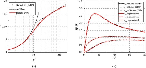
In the present work, the channel flow data generated by Kim et al. (1987) is used for the verification purpose for the incompressible flow solver. Figure 1(a) illustrates that the mean-velocity profile which is obtained by the method in the present work is in good agreement with that in the work of Kim et al. (1987). And the root-mean-square velocity fluctuations which are normalized by wall-shear velocity are compared with the data in the work of Kim et al. (1987), as shown in Figure 1(b). The nice matching can be observed in each sub-graph. Consequently, the comparisons indicate that the code is accurate and reliable for the simulations on the fully developed turbulent flow inside channels.

Figure 1. Comparison with the work of Kim et al. (1987). (a) Mean-velocity profile. (b) Root-mean-square velocity fluctuations.

3. Computational details

3.1. Computational domains

The flow geometry where the Navier–Stokes equations are solved and the coordinate system are demonstrated in Figure 2(a). In this work, x, y, and z denote three coordinates in space, and they are made non-dimensional with friction velocity, $u^{\ast }$, and ν. Hence, $x^{+}=u^{\ast }x/\nu$, $y^{+}=u^{\ast }y/\nu$, and $z^{+}=u^{\ast }z/\nu$. The upper wall is a no-slip flat plate, while the lower one is mounted with streamwise V-shape riblets. The flat surface is at $y=\delta$ and the riblet wall is located at $y=-\delta$. Subsequently, it becomes possible to compare the flows over the flat wall and the riblets at the same time according to Choi et al. (1993), Chu and Karniadakis (1993), and Goldstein et al. (1995).

Figure 2. Computational domain bounded by riblets surface and flat surface. (a) Computational domain and coordinates. (b) Cross-sectional view of the channel.

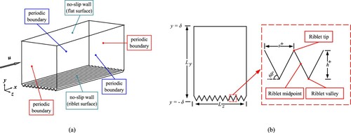
For symmetry V-shape riblets, the non-dimensional spacing, $s^{+}=u^{\ast }s/\nu$, is defined as the normalized crest-to-crest distance. Correspondingly, s represents the dimensional spacing. Similarly, the non-dimensional height, $h^{+}=u^{\ast }h/\nu$, denotes the normalized crest height, and h corresponds to the dimensional height. And the ridge angle, β, is defined as the angle between the inclined-wall and z-direction.

To determine the configuration, the spacing $s^{+}$ and the ridge angle β are needed. As the ridge angle is fixed at ${60}^{\circ }$ in the present work, $s^{+}$ is the only changeable parameter to control the shape of the riblets. And the cross-section of the channel is illustrated schematically in Figure 2(b). And the riblet tip is defined as the location at the peak of the V-shape riblet, midpoint represents the position at the mid-inclined-wall of the symmetry V-shape riblets, and riblet valley denotes the point at the bottom of the riblet.

Although sizes of computational domains may be different in different cases, the minimal domain of the channel has the dimensions $L_x\times L_y\times L_z=2\pi \delta \times 2\delta \times \frac{1}{2}\pi \delta$, where $L_x$, $L_y$ and $L_z$ denote the streamwise, normal, and spanwise length of the domain, respectively. And the size is larger than the minimum flow unit proposed by Jiménez and Moin (1991) for the studied Reynolds number, besides which the domain of the channel is larger than that of the work of Choi et al. (1993). Hence, the domain size is large enough to bound the fully developed turbulent flow.

3.2. Boundary and initial conditions

As for the boundary conditions, the upper wall (flat surface) and the lower wall (riblets) are both no-slip walls. In the x (streamwise) and z (spanwise) directions, the periodic boundary conditions are applied. And they are shown in Figure 2(a). The laminar flow is generated at the given Reynolds number in advance, and the laminar flow field is used as the initial state for the turbulence resolving. After adequate time steps, the fully developed turbulence is achieved, and the Reynolds number based on the bulk flow velocity is at the given level.

3.3. Computational grids

In the streamwise direction, a uniform mesh is used, and the spacing between adjacent grid points, $\mathrm{\Delta }{x}^{+}$, is 0.80. Similarly, in the spanwise direction, the uniform mesh on the riblet wall is also applied, and $\mathrm{\Delta }{z}^{+}$ denotes the corresponding distance between adjacent nodes. In the wall-normal direction, non-uniform grids are placed by hyperbolic tangent distribution. In addition, the distance between the grid point and the wall, $\mathrm{\Delta }{y}^{+}$, is 0.90. The parameters for the numerical simulations are shown in Table 2, where $N_1$, $N_2$, and $N_3$ represent the number of nodes in streamwise, normal, and spanwise directions, respectively.

Table 2. Parameters for numerical investigations of turbulent flows.

Case	$s^{+}$	$h^{+}$	$N_1\times N_2\times N_3$	$\mathrm{\Delta }{x}^{+}$	$\mathrm{\Delta }{y}^{+}$	$\mathrm{\Delta }{z}^{+}$
$\mathrm{A}$	10.87	$9.41$	$401\times 201\times 769$	0.8	0.9	0.41
$\mathrm{B}$	12.54	10.85	$401\times 201\times 673$	0.8	0.9	0.46
$\mathrm{C}$	14.61	12.65	$401\times 201\times 649$	0.8	0.9	0.48
$\mathrm{D}$	16.30	14.12	$401\times 201\times 577$	0.8	0.9	0.54
$\mathrm{E}$	18.81	16.29	$401\times 201\times 505$	0.8	0.9	0.62
$\mathrm{F}$	21.94	19.01	$401\times 201\times 481$	0.8	0.9	0.65
$\mathrm{G}$	23.93	20.72	$401\times 201\times 441$	0.8	0.9	0.71
$\mathrm{H}$	26.22	22.71	$401\times 201\times 401$	0.8	0.9	0.78
$\mathrm{I}$	29.57	25.61	$401\times 201\times 361$	0.8	0.9	0.87
$\mathrm{J}$	32.80	28.40	$401\times 201\times 321$	0.8	0.9	0.98
$\mathrm{K}$	37.61	32.57	$401\times 201\times 281$	0.8	0.9	1.11
$\mathrm{L}$	44.05	38.15	$401\times 201\times 241$	0.8	0.9	1.30

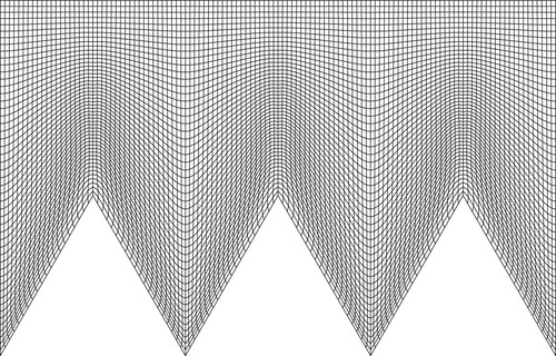
Hence, the meshes are finer than the numerical investigations of Chu and Karniadakis (1993) and Choi et al. (1993) in all directions. The computational grid distributions over the riblets are shown in Figure 3 and parameters of the mesh in each case are illustrated in Table 2.

Figure 3. Computational grids near the riblets.

3.4. Mesh dependence check

A numerical simulation of the case where the spacing $s^{+}=16.30$ is picked to check the mesh sensitivity. The number of grid points in stream wise, spanwise and normal direction is raised 1.5 times, and the drag-reducing effects of the riblets is changed by less $1\mathrm{\%}$. And the results are shown in Table 3.

Table 3. Parameters for numerical investigations of turbulent flows.

Case	$N_1\times N_2\times N_3$	Drag-reducing effect
$\mathrm{A}$	$401\times 201\times 481$	$5.6400\mathrm{\%}$
$\mathrm{B}$	$601\times 201\times 481$	$5.6323\mathrm{\%}$
$\mathrm{C}$	$401\times 301\times 481$	$5.6596\mathrm{\%}$
$\mathrm{D}$	$401\times 201\times 721$	$5.6952\mathrm{\%}$

In each simulation, the Reynolds number based on the channel half-height and centerline velocity is 5000. The global time steps are set constant at 0.001, and the global CFL number based on the minimal grid spacing is fixed at approximately 0.2. The cases are performed on 10 cluster nodes with 24 Intel Xeon E5-2670 cores in each node, and the nodes are connected by the InfiniBand (IB). In each simulation, the total number of time step is at least 5 million.

4. Computational results

As the governing equations are integrated in time, the data of the turbulent flow field will be gathered once the velocity field becomes statistically steady. For mean flow, the total averaging time is $500\delta /U_l$ for all results. To demonstrate the equilibrium states, the time history of wall-shear rates at the flat wall and riblets ($s^{+}=21.94$ and 44.05) are demonstrated in Figure 4.

Figure 4. History of wall-shear rates in 500 non-dimensional time steps.

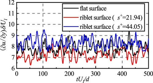
Figure 4 suggests that the statistically steady state is achieved after a large number of steps. In the following parts, drag-reducing performances of riblets with different $s^{+}$ are compared. Subsequently, the drag-reducing effects in different cases are illustrated and compared. Then the detailed data about mean-flow properties and turbulence statistics are analyzed. And visualizations of flow fields are demonstrated. Finally, drag-reducing mechanisms of riblets are discussed.

4.1. Wall-shear stress reduction

To evaluate the effects on viscous drag reduction, wall-shear stress is calculated. Then the formula is as following: (16) ${\tau }_{{}_w}=\mu {\left(\frac{\mathrm{\partial }u}{\mathrm{\partial }n}\right)}_{y=0}$(16) where ${\tau }_{{}_w}$ denotes the wall-shear stress, and n denotes the coordinate normal to the surface. Hence, the area of the riblet surface is $1/\cos (\alpha )$ times larger than the flat plate. The drag reduction ratio is used and the formulation is as the following. (17) ${\eta }_{\tau }=\frac{{\tau }_{{}_{\mathrm{Riblets}}}-{\tau }_{{}_{\mathrm{FlatSurface}}}}{{\tau }_{{}_{\mathrm{FlatSurface}}}}\times 100\mathrm{\%}$(17) where ${\tau }_{{}_{\mathrm{Riblets}}}$ denotes the wall-shear stress for the riblet wall and ${\tau }_{{}_{\mathrm{FlatSurface}}}$ represents that corresponding to the flat plate.

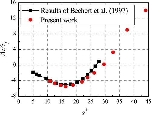
After calculation, the result is compared with the experimental data of Bechert et al. (1997), as shown in Figure 5. The diagram illustrates that the drag reduction ratio of the riblet surface increases to $5.61\mathrm{\%}$, as $s^{+}$ increases to 16.10. Then the ratio begins to decline and continues on this downward turn. Finally, the drag of the riblet surface goes larger than that acted on the flat plate, namely, the drag-reducing effect vanishes. In the following sections, For the sake of simplicity, two distinguished cases are analyzed and discussed. One is the drag-decreasing case ($s^{+}=21.94$) and the ratio is $4.27\mathrm{\%}$. This case is an example of the drag-reducing cases. The other one corresponding to the drag-increasing effect is the case where $s^{+}=44.05$ and there is an $13.90\mathrm{\%}$ increase in drag.

Figure 5. Comparison of the drag-reducing performance with the work of Bechert et al. (1997).

4.2. Mean-flow velocity

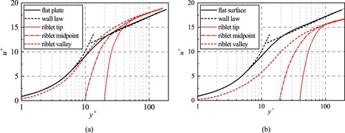
To demonstrate more detailed information on the properties of the mean velocity, the profiles normalized by local wall-shear velocity in the drag-decreasing case ($s^{+}=21.94$) and drag-decreasing case ($s^{+}=21.94$) are displayed in Figure 6. In the drag-decreasing case, the logarithmic region of the turbulent boundary layer is shifted, while there is a download shift in that for the drag-increasing case. Sub-graph 6(a) reveals the mean-velocity profiles over the riblet tips encounter those over the midpoint and valley in the buffer layer, while for the drag-increasing riblets (as shown in sub-graph 6(b)), the profiles coincide from the log-layer region. This phenomenon indicates that for each case there is a certain position below which the influences of different parts of the riblets on the flow are different. Therefore, for drag-decreasing cases and drag-increasing cases, the spanwise inhomogeneity caused by riblets affects the flow significantly. And the position in the drag-increasing case is higher than that in the drag-decreasing case.

Figure 6. Mean-velocity profile in wall units over the different locations of the riblets in the drag-decreasing case ($s^{+}=21.94$) and drag-increasing case ($s^{+}=44.05$). (a) The drag-decreasing case. (b) The drag-increasing case.

4.3. Turbulent intensity

Turbulent intensity is used to estimate the level of velocity fluctuations and in this section, the root-mean-square (RMS) velocity is normalized by the wall-shear velocity. As shown in Figure 7, the three components of the turbulence intensities over the drag-decreasing riblets ($s^{+}=21.94$), drag-increasing riblets ($s^{+}=44.05$), and flat plate surface are compared.

Figure 7. Root-mean-square velocity fluctuations over the riblet tip, midpoint and valley in the drag-decreasing case ($s^{+}=21.94$) and drag-increasing case ($s^{+}=44.05$). (a) The drag-decreasing case. (b) The drag-increasing case.

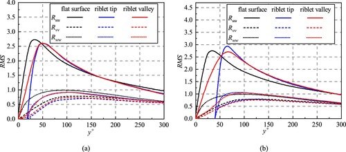
Compared to the flat plate, there is a decline in each component of the turbulent intensity in the drag-decreasing case ($s^{+}=21.94$). An approximately $10\mathrm{\%}$ reduction is obtained for the spanwise RMS velocity fluctuation and about $7\mathrm{\%}$ is for the streamwise component. In the drag-increasing case ($s^{+}=44.05$), compared to the flat side, the streamwise component over the riblets increases by around $5\mathrm{\%}$ while there exists a small drop for this component over riblet valleys. For the normal component, the turbulent intensity increases a little.

Therefore, the drag-decreasing riblets can weaken the turbulent intensities over the riblets, which is beneficial for drag reduction. Meanwhile, the riblet surface is not flat and it increases the wetted area (from Equation (16(16) ${\tau }_{{}_w}=\mu {\left(\frac{\mathrm{\partial }u}{\mathrm{\partial }n}\right)}_{y=0}$(16) )), which is bad for drag reduction. For the drag-decreasing case, the effect of restraint of the turbulent intensity suppresses the effect of the area increasing, which leads to the friction drag reduction. This phenomenon in the present work is in good agreement with those of Choi et al. (1993) and Goldstein et al. (1995). And this phenomenon will be analyzed and discussed from other aspects in the following sections.

4.4. Vorticity

In turbulent flow, the fluid is always rational and vorticity can be used to evaluate the rotation. Vorticity is defined as the curl of the velocity $\mathit{v}$, namely, (18) $\mathit{\omega }=\mathrm{\nabla }\times \mathit{v}$(18) It is known that the large-scale streamwise vortices are associated with the Reynolds shear stress and turbulent energy production according to Pope (2000). This section compares the vorticity fluctuations over drag-decreasing riblets, drag-increasing riblets, and the flat wall. And the root-mean-square fluctuations of vorticity in wall units are illustrated in Figure 8.

Figure 8. The root-mean-square fluctuations of vorticity in wall coordinates in the drag-decreasing case ($s^{+}=21.94$) and drag-increasing case ($s^{+}=44.05$). (a) x-vorticity in the drag-decreasing case. (b) x-vorticity in the drag-increasing case. (c) y-vorticity in the drag-decreasing case. (d) y-vorticity in the drag-increasing case. (e) z-vorticity in the drag-decreasing case. (f) z-vorticity in the drag-increasing case.

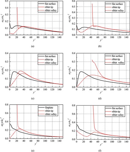
From Figure 8, in the drag-decreasing case ($s^{+}=21.94$), ${\omega }_x$ reaches the maximum around tips of riblets, then there is a decline. This indicates that centers of large-scale vortices stay near riblet tips, which is in accordance with phenomena described by Choi et al. (1993) and Kim et al. (1987). Compared to the flat surface, the vorticity fluctuations above the riblet surface are weakened, and the intensity of x-vorticity decreases by $14.21\mathrm{\%}$ (the number is $12\mathrm{\%}$ in the work of Choi et al. (1993)). In the drag-increasing case ($s^{+}=44.05$), the vorticity fluctuates more seriously (compared with the flat plate). And the location where x-vorticity achieves the maximum is lower than the riblet tip, which indicates that the vortices reside in the valleys. The phenomenon indicates that the flow in the riblets is fairly rotational and swirling. Hence, the distinct events in the two cases demonstrate that the drag-decreasing riblets could weaken the interactions between the streamwise vortices and the riblet surface and make the fluid inside the riblets more irrotational.

4.5. Reynolds shear stress analysis

The Reynolds shear stress is defined as the velocity covariances, namely, $-⟨u^{\mathrm{\prime }}{v}^{\mathrm{\prime }}⟩$. And in this section, the $-⟨u^{\mathrm{\prime }}{v}^{\mathrm{\prime }}⟩$ profiles in wall units over drag-decreasing riblets ($s^{+}=21.94$), the drag-increasing case ($s^{+}=44.05$) and the smooth surface are plotted, as shown in Figure 9.

Figure 9. Reynolds shear stress over the riblets in the drag-decreasing case ($s^{+}=21.94$) and drag-increasing case ($s^{+}=44.05$). (a) The drag-decreasing case. (b) The drag-increasing case.

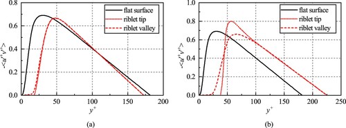
For the drag-decreasing case ($s^{+}=21.94$) as shown in Figure 9(a), the profiles over the riblet tip and valley coincide and overlap further away from the buffer layer. And the Reynolds shear stresses decrease to 0 around the centerline. This suggests that the fluid over one wall of the channel does not affect the Reynolds shear stress at the opposite side, which is consistent with the work of Antonia et al. (1992). Compared with the flat plate, a maximum of $14.34\mathrm{\%}$ reduction of Reynolds shear stress is obtained, and the number is $16\mathrm{\%}$ in the work of Walsh (1980) and $12\mathrm{\%}$ according to Choi et al. (1993). In the drag-increasing case ($s^{+}=44.05$) as shown in Figure 9(b), compared with the flat plate, the Reynolds shear stress above the riblets tips increase by $10\mathrm{\%}$, while the quantity above the valley decreases a little. And Reynolds shear stresses over the riblets also drop to 0 at the centerline and this is the same as the drag-decreasing case.

4.6. Skewness and flatness

In this section, skewness factors and flatness factors of the velocity fluctuations are computed. The skewness and flatness are the third standardized moment and the fourth moment according to Pope (2000). The skewness and flatness factors of the three components (streamwise, normal, spanwise) in global coordinates are demonstrated in Figures 10 and 11, respectively.

Figure 10. Skewness factors in the drag-decreasing case ($s^{+}=21.94$) and drag-increasing case ($s^{+}=44.05$). (a) The drag-decreasing riblet valley. (b) The drag-decreasing riblet tip. (c) The drag-increasing riblet valley. (d) The drag-increasing riblet tip.

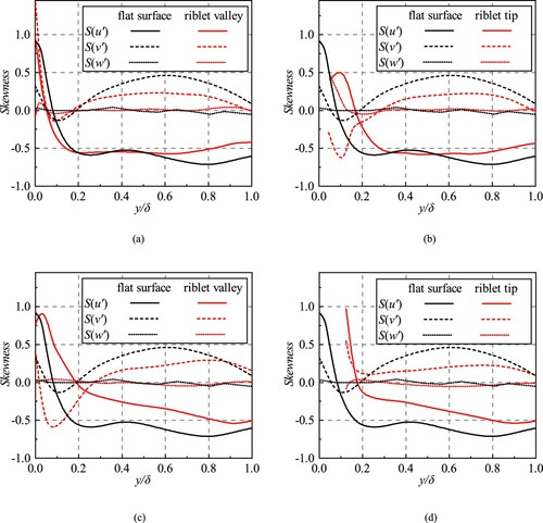
Figure 11. Flatness factors in the drag-decreasing case ($s^{+}=21.94$) and drag-increasing case ($s^{+}=44.05$). (a) The drag-decreasing riblet valley. (b) The drag-decreasing riblet tip. (c) The drag-increasing riblet valley. (d) The drag-increasing riblet valley.

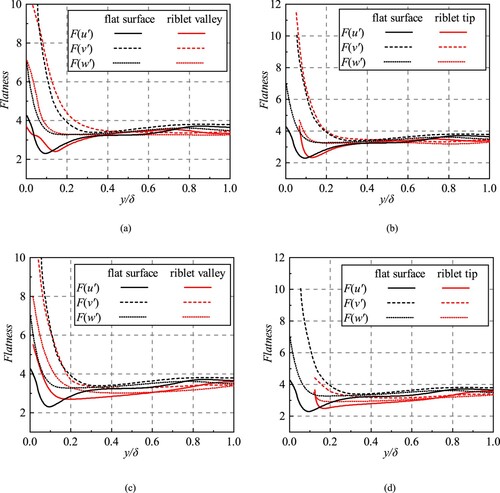
Figure 10 demonstrates the profiles of skewness factors over the flat surface, drag-deceasing riblets ($s^{+}=21.94$) and the drag-increasing riblets ($s^{+}=44.05$). Compared with the flat surface, the skewness of $u^{\mathrm{\prime }}$ and $v^{\mathrm{\prime }}$ in the drag-decreasing case and the drag-increasing case changed significantly. In the drag-decreasing, the skewness of $u^{\mathrm{\prime }}$ declines near the valley while there is an increase above the tip. And the Skewness of $v^{\mathrm{\prime }}$ rises near the valley and tip. In the drag-increasing case, skewness factors of $u^{\mathrm{\prime }}$ and $v^{\mathrm{\prime }}$decrease near the valley while the two parameters increase near the tip. In the two cases, the skewness of $w^{\mathrm{\prime }}$ is hardly modified.

For the flatness factors, in the drag-decreasing case, the three components are modified slightly near the valley and tip. And in the drag-increasing case, the flatness factors of $u^{\mathrm{\prime }}$ and $w^{\mathrm{\prime }}$ increase above the valley and tip, while there is a decline in the flatness of $v^{\mathrm{\prime }}$ near the valley and the tip.

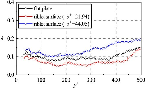
4.7. Behaviors of streamwise vortices above the riblets

It was mentioned that large-scale streamwise vortices interacted with the wall frequently which led to the production of Reynolds shear stress and the drag increases. Densities and distributions of vortices over the riblets can also affect the Reynolds shear stress and turbulent intensities. In this section, the distributions of the streamwise vortices above riblets in the drag-decreasing ($s^{+}=21.94$) and the drag-increasing ($s^{+}=44.05$) are examined. The method to obtain the population density of streamwise vortices proposed by Wu and Christensen (2006) is performed in this work. The population density, ${\Pi }_p$, is defined as the ensemble-averaged number of the streamwise vortices in a rectangular area of wall-normal height $\mathrm{\Delta }{y}_p$ and spanwise width $\mathrm{\Delta }{z}_p$ centered at y, as shown in the following, (19) ${\Pi }_p\left({\displaystyle \frac{y}{\delta }}\right)=\frac{N_p\left({\displaystyle \frac{y}{\delta }}\right)}{{\displaystyle \frac{\mathrm{\Delta }{y}_p}{\delta }{\displaystyle \frac{\mathrm{\Delta }{z}_p}{\delta }}}}$(19) where $\mathrm{\Delta }{y}_p$ and $\mathrm{\Delta }{z}_p$ denote the non-dimensional normal height and spanwise height of the rectangular area, respectively. $N_p(\frac{y}{\delta })$ represents the number of vortices whose centers are located inside the rectangular area. To ensure that the area can accommodate the large-scale streamwise vortices, the size needs to be large enough, and in this work, $\mathrm{\Delta }{y}_p=20$, $\mathrm{\Delta }{z}_p=20$. Figure 12 demonstrates the population densities over the flat surface, drag-reducing riblets, and drag-increasing ones.

Figure 12. Distributions of the large-scale streamwise vortices over riblets.

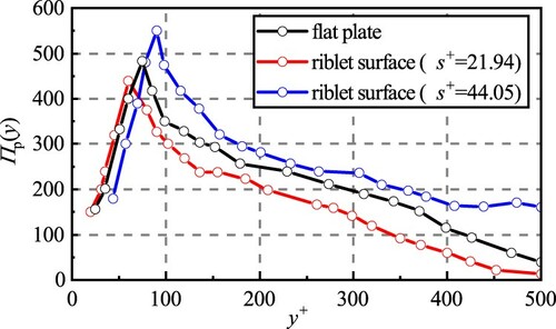
From Figure 12, in each case, the number of the vortices increases significantly around the surface, subsequently, there exists a maximum number of streamwise vortices at the log layer. And in the drag-decreasing case ($s^{+}=21.94$), the number is the smallest, while that in the drag-increasing case ($s^{+}=44.05$) is the largest. In the drag-decreasing case, the maximum value occurs at around $y^{+}=70$, which is the closest to the wall. For the drag-increasing case, the position of the maximum is at $y^{+}=80$, which is the farthest from the wall. After that, the number of vortices declines gradually in each case. The number of vortices over drag-increasing riblets still suppresses those in the other two cases, and the number in the drag-decreasing case is the smallest.

In conclusion, the drag-decreasing riblets can lower the number of vortices over the riblets while there is an increase in the number in the drag-increasing case. In the drag-decreasing case, the drop in the number of streamwise vortices also causes less frequent interactions between vortices and the riblet surface. And this may be regarded as one possible reason for the drag-reducing effects of riblets.

To illustrate the distributions of streamwise vortices visually, the locations of vortices in the drag-decreasing ($s^{+}=21.94$) and drag-increasing ($s^{+}=44.05$) cases are drawn in Figure 13. For the two distinguished cases, locations of streamwise vortices of 300 instantaneous velocity fields are gathered and plotted. The positions of vortices are determined by the maximum value of the vorticity according to Lee and Lee (2001). Moreover, the number of riblets which are displayed in Figure 13(a) is the same as that in Figure 13(b), while the ranges in $y^{+}$ and $z^{+}$ axes are different in the cases. So the displayed area in the case of $s^{+}=21.94$ ($\mathrm{\Delta }{z}^{+}\times \mathrm{\Delta }{y}^{+}=87.76\times 50.00$) is smaller than that ($\mathrm{\Delta }{z}^{+}\times \mathrm{\Delta }{y}^{+}=176.20\times 100.00$) in the case where $s^{+}=44.05$.

Figure 13. Locations of large-scale streamwise vortices above riblets in the drag-decreasing case ($s^{+}=21.94$) and drag-increasing case ($s^{+}=44.05$).

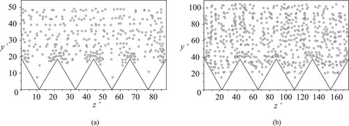
From Figure 13, it is clear that large-scale streamwise vortices over drag-decreasing riblets (Figure 13(a)) are less than those over drag-increasing riblets (Figure 13(b)). In the drag-decreasing case, streamwise vortices are mainly situated around riblet tips and they hardly stay in the riblets. So the vortices interact with riblet tips frequently and the fluid inside the riblets goes smoothly. These events also generate secondary flows. For the drag-increasing case corresponding to the wider spacing, the large-scale streamwise vortices are narrower than the riblets so that the vortices can reach the valleys and contact with all parts of the riblet surface. These events make the Reynolds shear stress increase and contribute to the production of turbulent energy.

Streamwise vortices are the large-scale turbulence structure, and the behaviors of them are relative to the shear stress. Consequently, contributions of the vortices to the overall mean shear are generated. The total mean shear is (20) $\tau (y)=\mu \frac{\mathrm{\partial }U}{\mathrm{\partial }y}-\rho ⟨u^{\mathrm{\prime }}{v}^{\mathrm{\prime }}⟩$(20) Where the term $\mu \frac{\mathrm{\partial }U}{\mathrm{\partial }y}$ denotes the mean viscous shear, and $\rho ⟨u^{\mathrm{\prime }}{v}^{\mathrm{\prime }}⟩$ represents the contributions of the turbulent stresses. In this work, the contributions of the streamwise vortices to mean shear can be computed as the stress fraction which is given by (21) $S_p(y)=\frac{{\tau }_p(y)}{\tau (y)}$(21) where ${\tau }_p(y)$ denotes the contributions of the streamwise vortices. To obtain the terms in Equation (21(21) $S_p(y)=\frac{{\tau }_p(y)}{\tau (y)}$(21) ), the techniques proposed by Wu and Christensen (2006) are employed in this work. Then, the contributions of the streamwise vortices above the drag-decreasing riblets, flat plate, and drag-increasing riblets are illustrated in Figure 14.

Figure 14. Contributions of the large-scale streamwise vortices to overall mean shear.

From Figure 14, it is illustrated that the ratio of contributions of the streamwise vortices over the drag-decreasing riblets is the smallest while the number in the drag-increasing case is the largest. And this phenomenon is consistent with the distributions of the vortices near the wall in the cases. This indicates that the increase in the number of vortices leads to the rise of the wall-shear stress, which causes a larger drag.

4.8. Instantaneous velocity field visualization

To show the instantaneous flow field visually, the contour diagrams of the u component of velocity and the velocity vector of crossflow for both drag-decreasing case ($s^{+}=21.94$) and drag-increasing case ($s^{+}=44.05$) are demonstrated in Figure 15. From the near-wall turbulent structures, the differences between the two distinguished cases can be examined.

Figure 15. Contour diagrams of the u component of velocity in the drag-decreasing case ($s^{+}=21.94$) and drag-increasing case ($s^{+}=44.05$). (a) The drag-decreasing case. (b) The drag-increasing case.

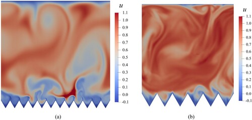
Figure 15 illustrates instantaneous flow fields in both cases. It is noted that, with the development of turbulence, the flow in the channel will be affected by riblets, so the velocity at some positions will be larger than 1.0. From Figure 15(a), in the drag-decreasing case ($s^{+}=21.94$), the flow goes smoothly in the riblets and the fluid inside the riblets is steady. In the drag-increasing case ($s^{+}=44.05$) as demonstrated in Figure 15(b), the high-speed outer flow can enter the riblets and the streamwise vortices can interact with the valleys frequently. This causes the increase of the Reynolds shear stress.

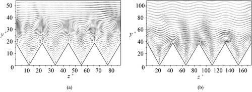
From the cross-flow velocity fields as shown in Figure 16, for the drag-decreasing case ($s^{+}=21.94$), the large-scale streamwise vortices are located around the riblet tips, on the other hand, the vortices arrive at the riblets valleys in the drag-increasing case ($s^{+}=44.05$). And in the drag-decreasing case, it can be observed the cross-flow velocity vectors are nearly zero in valleys, which means that the v component and w component of the velocity vector are very small and the fluid inside the valleys moves almost along x axis. So the phenomenon suggests that the flow inside the riblet valleys is smooth and the fluid does not interact with the surface violently. In addition, the spanwise motions of large-scale streamwise vortices are weakened, and the vortices are anchored on the riblet surface.

Figure 16. Cross-flow velocity fields, $(v,w)$, in the drag-decreasing case ($s^{+}=21.94$) and drag-increasing case ($s^{+}=44.05$). (a) The drag-decreasing case. (b) The drag-increasing case.

5. Aerodynamic force measurements

From the numerical simulations, the riblet side of the channel in numerical simulations can be regarded as a local part of a 3-dimensional configuration at lower AoAs. Besides, the flow is anchored on the surface by riblets, and this will affect the flow separation at moderate AoAs. Consequently, in this section, performances of riblets on the drag acted on a transport model are evaluated experimentally in a low-speed wind tunnel. All experiments are carried out in a $1.8\mathrm{m}\times 1.4\mathrm{m}$ closed-circuit wind tunnel in China Aerodynamics Research and Development Center. The speed ranges between 20 to 70 m/s with a 10 m/s interval. The testing AoAs are modified from $-2^{\circ }$ to ${20}^{\circ }$, which corresponds to a $2^{\circ }$ interval.

5.1. Models

The model of a transport aircraft is a mid-sized, 1/40 scaling, commercial transport aircraft with two engines. In the experiments, the engines are not installed. The model contains fuselage, wings, horizontal stabilizers and vertical stabilizers. To compare the effectiveness of riblets with smooth surface, two models are manufactured, as shown in Figure 17.

Figure 17. The transport models with smooth surface and riblet surface.

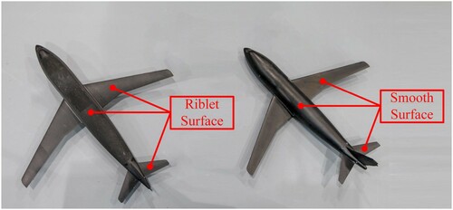
One is the original baseline model, of which surface is smooth, while the other one is mounted with riblets. The material of the models is aluminum alloy and the riblets are created by milling operation directly. Each component of the riblet model is mounted with riblets, including fuselage, wings, horizontal stabilizers, and vertical stabilizers. To adapt the shape change of the fuselage, the width of the riblet will change. For the aircraft model in this work, the spacing of the riblet is 0.7 mm at the head of the fuselage, and the spacing is 0.30 mm at the end. At wings and most areas of the fuselage, the spacing is 0.41 mm, correspondingly, the height is 0.36 mm. The basic geometric parameters of the model are illustrated in Table 4.

Table 4. Parameters of the transport model.

Parameters		Value (m)
Fuselage	Equivalent diameter	0.09441
	Length	$0.75680$
Wing	MAC^a	0.09286
	Span	0.74640
	Area	0.07440
Horizontal stabilizer	MAC	$0.04881$
	Span	$0.24880$
Vertical stabilizer	MAC	$0.07920$
	Span	$0.11920$

Note:^aMAC: the mean aerodynamic chord.

For the riblet in this work, the Reynolds number based on the spacing of the riblet varies between 310 to 1103. During a wing tunnel run, the pressure in the test chamber is 100026 Pa, and the temperature is 333 K. Hence, the Reynolds number of the wing-body based on the wingspan ranges between $7.69\times {10}^5$ to $2.69\times {10}^6$. For the wing-body model, the height of the riblets at wings and most areas of the fuselage is 0.36 mm. Hence, the Reynolds number based on the size ranges between 356 to 1246. So the variation of the studied Reynolds number in most of the numerical cases stays within the range of Reynolds number changes in the experiment.

5.2. Experiment setup

The experiment is conducted in a closed-circuit wind tunnel with a maximum airflow speed of 130 m/s in China Aerodynamics Research and Development Center, as shown in Figure 18. And more detailed information on the wind tunnel is shown in Table 5.

Figure 18. Schematic diagram of the wind tunnel.

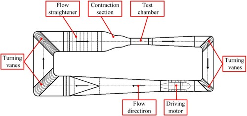
Table 5. Parameters of the low-speed wind tunnel.

Parameters	Value
Dimensions (m)	$1.8\times 1.4$
Wind speed (m/s)	$20\sim 130$
Angle of attack (${}^{\circ }$)	$-20\sim 30$
Dynamic pressure stability	$0.20\mathrm{\%}$
Turbulence intensity	$0.08\mathrm{\%}$

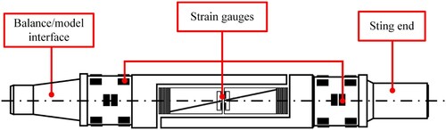
To measure aerodynamic loads acting on models, an internal six-component strain stress balance is employed, as shown in Figure 19. The balance is installed inside the model, therefore there is no interference which is introduced by components of the balance. In this work, the range and resolution of the balance are selected according to the expected aerodynamic load.

Figure 19. Schematic diagram of the six-component internal strain guage balance.

Before the test, several steps for calibration are carried out to ensure that the balance can resolve each component of aerodynamic loads accurately. In this work, the ratio of the difference between computed loads and the real value to the balance scale is defined as the accuracy. And the accuracy of the balance is better than $0.2\mathrm{\%}$ (Figure 20).

Figure 20. Model installation in the wind tunnel.

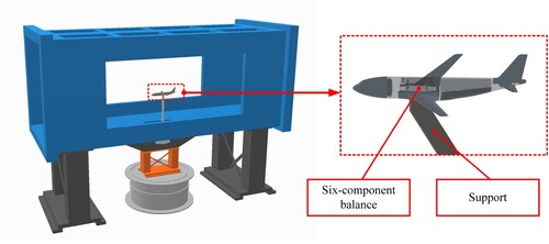
The testing model was mounted on the six-component balance, and it was set in the horizontal position, as shown in Figure 20. The balance is inside the fuselage, and its electromechanical center coincides with the gravity center of the model. Both of them are installed on a support with NACA0012 airfoil. After installing and testing, the signals of the data acquisition system are recorded. Then, the wind tunnel begins to run. The aerodynamic characteristics of the two models are measured at speeds of $20\sim 70\mathrm{m}/\mathrm{s}$ with a 10 m/s interval. The range of the AoA is $-2^{\circ }\sim {20}^{\circ }$ with a $2^{\circ }$ interval. Hence, a total of 72 cases were tested for one model. Each state is measured three times, and an averaged result is obtained.

5.3. Results of the experiment

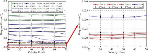
In this section, drag coefficients of the wing-body configuration mounted with riblets are compared with those of the baseline model, and the drag-reducing effect of riblets will be illustrated. The drag coefficient $C_D$ is defined as: (22) $C_D=\frac{D}{{\displaystyle \frac{1}{2}}\rho V^2{S}_w}$(22) where D denotes the aerodynamic drag obtained by the experiment, V represents the wind speed of the wind tunnel, and $S_w$ is the area of wings. The drag coefficients of the two models are illustrated in Figure 21. The red lines denote that, at the given AoA, the drag of the ribleted model is lower than that of the smooth model for all testing speeds. The green lines are corresponding to the cases where the drag of the ribleted model is larger than that of the smooth model. And the blue lines represent that both the drag-decreasing and drag-increasing effects exist within the speed range.

Figure 21. Drag coefficients of the experimental models.

To show the drag-reducing effect of riblets on the model clearly, the drag reduction ratio is employed. In this section, drag reduction ratio is defined, as shown in the following. (23) ${\eta }_{{}_D}=\frac{D_{{}_{\mathrm{Riblets}}}-D_{{}_{\mathrm{FlatSurface}}}}{D_{{}_{\mathrm{FlatSurface}}}}\times 100\mathrm{\%}$(23) where $D_{{}_{\mathrm{Riblets}}}$ represents the drag acted on the ribleted model and $D_{{}_{\mathrm{FlatSurface}}}$ denotes the drag corresponding to the smooth one. The drag-reducing effects of riblets on the aircraft are illustrated in Figure 22. Similarly, The red lines denote that, at the given AoA, riblets have drag-reducing effects for all testing speeds. The green lines correspond to the cases where the riblet surface increases the drag of the wing-body configuration. And the blue lines represent that the drag-decreasing and drag-increasing effects exist within the speed range. Figure 22(a) provides an overall view of the results, and the details are illustrated in Figure 22(b).

Figure 22. Drag-reducing effects of riblets on the aircraft. (a) Overall view of drag reduction ratio. (b) Details on drag-reducing ratio.

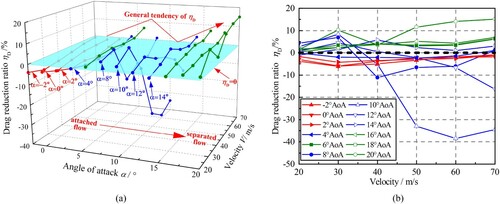
The result illustrates that a maximum of $39.8\mathrm{\%}$ drag reduction is obtained for the case where the angle of attack of the model is ${10}^{\circ }$ at 60 m/s. At lower angles of attack, the flow around the wings is unseparated, and the drag-reducing effect exists when the angle of attack ranges between $-2^{\circ }$ and $4^{\circ }$. However, at $6^{\circ }$ AoA, the drag is inclined. According to Zhang et al. (2018), for the case where the angle of attack is not too large, there is an increase in the pressure drag. At the same time, for the wing-body configuration, the existence of the pressure gradient will enhance the viscous drag reduction performance (Debisschop & Nieuwstadt, 1996). However, the two effects on drag reduction are opposite. Therefore, this indicates that, at $6^{\circ }$ AoA, the increase in pressure drag suppresses the performance of viscous drag reduction; hence the drag increases.

With the increase in AoA, the flow around the aircraft changes from an attached state to a separated state. And at moderate AoAs, the drag-reducing effects are obvious. According to the analysis of numerical results, the riblets make the fluid near the surface more irrotational, the Reynolds shear stress is lowered, and the spanwise motion of the large-scale vortices is inhibited. Hence, streamwise vortices are anchored and attached to the surface of the riblets. The effect of the riblets indicates flow separation will be weakened at moderate angles of attack. Consequently, the pressure drag will be reduced. This suggests that riblets on practical aircrafts can reduce both viscous drag and pressure drag at moderate AoAs. Due to the inhibition of flow separation, the drag-reducing performance of riblets on the wing-body configuration is enhanced.

6. Conclusions and discussions

Riblets, as one of the effective passive drag-reducing techniques for drag reduction, are investigated by direct numerical simulation and experiments in the present work. By the investigations, The conclusions are as the following.

• The method of the seventh WENO scheme, fractional-step time combined with LDDRK scheme, and the sixth compact schemes for the spatial discretization, time advancing, and viscous terms is of high accuracy for the resolution of incompressible turbulence flow over riblets.

• According to turbulence statistics of numerical simulation, for drag-decreasing cases and drag-increasing cases, the inhomogeneity of riblet affects the flow significantly. For drag-decreasing riblets, the effect is limited under the buffer layer, and it can hardly reach the outer layer.

• For behaviors of large-scale streamwise vortices, drag-decreasing riblets can keep streamwise vortices from valleys, thus the vortices are mainly situated around riblet tips. The spanwise motions of the streamwise vortices are weakened and the vortices are anchored at the riblet surface. In addition, there is a decrease in the population density of large-scale streamwise vortices near the wall and the ratio of contributions of the vortices to the total mean shear is reduced.

• In the force measurements, a maximum of $38.52\mathrm{\%}$ reduction in drag is achieved. For the aircraft at moderate angles of attack, because the flow over the riblet is more irrotational and the vortices are anchored at the wall, the separation of the boundary layer is weakened, and the flow attachment is enhanced. This indicates the there is also a decline in pressure drag.

Although the numerical and experimental results are obtained in this work, there are still drawbacks. The DNS method can clearly resolve the turbulence flow over the riblets, but the computational cost is too large. Hence, in the future, our group will focus on the construction of the riblet-equivalent boundary condition, which can estimate the aerodynamic forces rapidly. At the same time, our group will employ more advanced measurement techniques to study the turbulent flow and combine it with numerical methods to study the drag-reducing mechanisms.

Nomenclature

Latin characters

$a_l^k$	=	Lagrange interpolation coefficients in the WENO scheme
$C_k$	=	Ideal weights in the WENO scheme
$C_D$	=	Aerodynamic drag coefficient
D	=	Aerodynamic drag (N)
$D_{riblets}$	=	Aerodynamic drag acted on the aircraft mounted with riblets (N)
$D_{FlatSurface}$	=	Aerodynamic drag acted on the aircraft mounted with a smooth surface (N)
f	=	A function to be reconstructed in the WENO scheme
$f^{(1)}$	=	Derivative value of f
$F(\cdot )$	=	Flatness factors
h	=	Crest height normalized by centerline velocity
$h^{+}$	=	Crest height in wall units
$H_{j+1/2}^k$	=	Non-linear weights
$I{S}_k$	=	Smoothness measurements in the WENO scheme
$L_x$, $L_y$, $L_z$	=	Streamwise, normal and spanwise length of the channel
$N_1$, $N_2$, $N_3$	=	Number of nodes in the streamwise, normal, and spanwise direction
$N_p$	=	Number of vortices
p	=	Pressure (non-dimensional)
$\mathrm{\Delta }p$	=	Equivalent pressure drop in the channel flow (non-dimensional)
Q	=	Mass flow rate in channel flow (non-dimensional)
$Q^H$	=	Mass flow rate in intermediate steps (non-dimensional)
$Q^S$	=	Mass flow rate corresponding to the equivalent Stokes flow(non-dimensional)
$\mathrm{Re}$	=	Reynolds number
$R_{uu},R_{vv},R_{ww}$	=	Three components of root-mean-square velocity
s	=	Crest-to-crest distance normalized by centerline velocity
$s^{+}$	=	Crest-to-crest distance in wall units
$S(\cdot )$	=	Skewness factors
$S_p$	=	Contribution of the streamwise vortices to mean shear
$S_k$	=	Stencils of WENO scheme
$S_w$	=	Wing area (m${}^2$)
t	=	Time (non-dimensional)
$u_i$	=	Three components of the velocity field (non-dimensional)
$u_i^{(2)}$	=	Second derivated of $u_i$ (non-dimensional)
$u_i^F$	=	Instantaneous velocity vector field in channel flow (non-dimensional)
$u_i^H$	=	Velocity field in intermediate steps (non-dimensional)
$u_i^S$	=	Velocity field of equivalent Stokes flow (non-dimensional)
u, v, w	=	Three components of the velocity field of the flow field over riblets (non-dimensional)
$u^{\mathrm{\prime }},v^{\mathrm{\prime }},w^{\mathrm{\prime }}$	=	Three components of fluctuation velocity (non-dimensional)
$U_l$	=	Laminar centerline velocity in channel flow (m/s)
$u^{\ast }$	=	Friction velocity (m/s)
$\mathit{v}$	=	Velocity vector in the channel flow (non-dimensional)
V	=	Wind speed of wind tunnel (m/s)
$x_1,x_2,x_3$	=	Three coordinates in space in the WENO scheme (non-dimensional)
x, y, z	=	Three coordinates in space in channel flow
$x^{+},y^{+},z^{+}$	=	Non-dimensional coordinates in space in channel flow
$\mathrm{\Delta }{x}^{+},\mathrm{\Delta }{y}^{+},\mathrm{\Delta }{z}^{+}$	=	Spacing between adjacent grid points in the streamwise, normal, and spanwise direction
$\mathrm{\Delta }{y}_p$	=	Normal height of the area where the number of vortices is counted (non-dimensional)
$\mathrm{\Delta }{z}_p$	=	Spanwise height of the area where the number of vortices is counted (non-dimensional)

Greek characters

α	=	Angle of attack(${}^{\circ }$)
β	=	Ridge angle of the riblet (${}^{\circ }$)
δ	=	Channel half-height (m)
${\eta }_{{}_D}$	=	Drag reduction ratio
${\eta }_{\tau }$	=	Reduction ratio of wall-shear stress
μ	=	Dynamic viscosity (kg/m·s)
ν	=	Kinematic viscosity (m${}^2$/s)
${\mathrm{\Pi }}_p$	=	Population density of longitudinal vortices over walls
ρ	=	Fluid density (kg/m${}^3$)
$\tau (\cdot )$	=	Total mean shear (non-dimensional)
${\tau }_{{}_{FlatSurface}}$	=	Wall-shear stress of the smooth surface (non-dimensional)
${\tau }_p(\cdot )$	=	Contributions of streamwise vortices to total mean shear
${\tau }_{{}_{Riblet}}$	=	Wall-shear stress of the riblet surface (non-dimensional)
${\tau }_{{}_w}$	=	Wall-shear stress (non-dimensional)
$\mathit{\omega }$	=	Vorticity in the channel flow (non-dimensional)
${\omega }_{{}_k}$	=	Non-linear weight of the stencils in WENO scheme

Disclosure statement

No potential conflict of interest was reported by the author(s).

References

- Antonia R. A., Teitel M., Kim J., & Browne L. W. B. (1992). Low-Reynolds-number effects in a fully developed turbulent channel flow. Journal of Fluid Mechanics, 236, 579–605. https://doi.org/https://doi.org/10.1017/S002211209200154X
- Balsara D. S., & Shu C. -W. (2000). Monotonicity preserving weighted essentially non-oscillatory schemes with increasingly high order of accuracy. Journal of Computational Physics, 160(2), 405–452. https://doi.org/https://doi.org/10.1006/jcph.2000.6443
- Bechert D. W., Bruse M., Hage W. V., Vander Hoeven J. G. T., & Hoppe G. (1997). Experiments on drag-reducing surfaces and their optimization with an adjustable geometry. Journal of Fluid Mechanics, 338, 59–87. https://doi.org/https://doi.org/10.1017/S0022112096004673
- Choi H., Moin P., & Kim J. (1993). Direct numerical simulation of turbulent flow over riblets. Journal of Fluid Mechanics, 255, 503–539. https://doi.org/https://doi.org/10.1017/S0022112093002575
- Chu D. C., & Karniadakis G. E. (1993). A direct numerical simulation of laminar and turbulent flow over riblet-mounted surfaces. Journal of Fluid Mechanics, 250, 1–42. https://doi.org/https://doi.org/10.1017/S0022112093001363
- Coustols E., & Schmitt V. (1990). Synthesis of experimental riblet studies in transonic conditions. In Turbulence Control by Passive Means (pp. 123–140). Springer.
- Debisschop J., & Nieuwstadt F. (1996). Turbulent boundary layer in an adverse pressure gradient-effectiveness of riblets. AIAA Journal, 34(5), 932–937. https://doi.org/https://doi.org/10.2514/3.13170
- Ghalandari M., Bornassi S., Shamshirband S., Mosavi A., & Chau K. W. (2019). Investigation of submerged structures' flexibility on sloshing frequency using a boundary element method and finite element analysis. Engineering Applications of Computational Fluid Mechanics, 13(1), 519–528. https://doi.org/https://doi.org/10.1080/19942060.2019.1619197
- Goldstein D., Handler R., & Sirovich L. (1995). Direct numerical simulation of turbulent flow over a modeled riblet covered surface. Journal of Fluid Mechanics, 302, 333–376. https://doi.org/https://doi.org/10.1017/S0022112095004125
- Guangyao C., Chong P., Di W., Qingqing Y. E., & Jinjun W. A. N. G. (2019). Effect of drag reducing riblet surface on coherent structure in turbulent boundary layer. Chinese Journal of Aeronautics, 32(11), 2433–2442. https://doi.org/https://doi.org/10.1016/j.cja.2019.04.023
- Harten A., & Osher S. (1987). Uniformly high-order accurate nonoscillatory schemes. I. SIAM Journal on Numerical Analysis, 24(2), 279–309. https://doi.org/https://doi.org/10.1137/0724022
- Hossain S., Husain A., & Kim K.-Y. (2011). Optimization of micromixer with staggered herringbone grooves on top and bottom walls. Engineering Applications of Computational Fluid Mechanics, 5(4), 506–516. https://doi.org/https://doi.org/10.1080/19942060.2011.11015390
- Hu F. Q., Hussaini M. Y., & Manthey J. L. (1996). Low-dissipation and low-dispersion Runge–Kutta schemes for computational acoustics. Journal of Computational Physics, 124(1), 177–191. https://doi.org/https://doi.org/10.1006/jcph.1996.0052
- James G. C., & Dan M. S. (2020). Design of a slotted, natural-laminar-flow airfoil for commercial transport applications. Aerospace Science and Technology, 106, 106217. https://doi.org/https://doi.org/10.1016/j.ast.2020.106217
- Jiang G.-S., & Shu C.-W. (1996). Efficient implementation of weighted eno schemes. Journal of Computational Physics, 126(1), 202–228. https://doi.org/https://doi.org/10.1006/jcph.1996.0130
- Jiménez J., & Moin P. (1991). The minimal flow unit in near-wall turbulence. Journal of Fluid Mechanics, 225, 213–240. https://doi.org/https://doi.org/10.1017/S0022112091002033
- Kim J., & Moin P. (1985). Application of a fractional-step method to incompressible Navier-Stokes equations. Journal of Computational Physics, 59(2), 308–323. https://doi.org/https://doi.org/10.1016/0021-9991(85)90148-2
- Kim J., Moin P., & Moser R. (1987). Turbulence statistics in fully developed channel flow at low Reynolds number. Journal of Fluid Mechanics, 177, 133–166. https://doi.org/https://doi.org/10.1017/S0022112087000892
- Lee S.-J., & Lee S.-H. (2001). Flow field analysis of a turbulent boundary layer over a riblet surface. Experiments in Fluids, 30(2), 153–166. https://doi.org/https://doi.org/10.1007/s003480000150
- Lei D., & Lixin C. (2015). Effects of residual riblets of impeller's hub surface on aerodynamic performance of centrifugal compressors. Engineering Applications of Computational Fluid Mechanics, 9(1), 99–113. https://doi.org/https://doi.org/10.1080/19942060.2015.1004813
- Li W. (2020). Turbulence statistics of flow over a drag-reducing and a drag-increasing riblet-mounted surface. Aerospace Science and Technology, 104, 106003. https://doi.org/https://doi.org/10.1016/j.ast.2020.106003
- Liu X.-D., Osher S., & Chan T. (1994). Weighted essentially non-oscillatory schemes. Journal of Computational Physics, 115(1), 200–212. https://doi.org/https://doi.org/10.1006/jcph.1994.1187
- Luchini P., Manzo F., & Pozzi A. (1991). Resistance of a grooved surface to parallel flow and cross-flow. Journal of Fluid Mechanics, 228, 87–109. https://doi.org/https://doi.org/10.1017/S0022112091002641
- Nagarajan S., Lele S. K., & Ferziger J. H. (2003). A robust high-order compact method for large eddy simulation. Journal of Computational Physics, 191(2), 392–419. https://doi.org/https://doi.org/10.1016/S0021-9991(03)00322-X
- Pope S. B. (2000). Turbulent flows. Cambridge University Press.
- Salih S. Q., Aldlemy M. S., Rasani M. R., Ariffin A. K., Ya T. M. Y. S. T., Al-Ansari N., Yaseen Z. M., & Chau K. -W. (2019). Thin and sharp edges bodies-fluid interaction simulation using cut-cell immersed boundary method. Engineering Applications of Computational Fluid Mechanics, 13(1), 860–877. https://doi.org/https://doi.org/10.1080/19942060.2019.1652209
- Song X., Qi Y., Zhang M., Zhang G., & Zhan W. (2019). Application and optimization of drag reduction characteristics on the flow around a partial grooved cylinder by using the response surface method. Engineering Applications of Computational Fluid Mechanics, 13(1), 158–176. https://doi.org/https://doi.org/10.1080/19942060.2018.1562382
- Suzuki Y., & Kasagi N. (1994). Turbulent drag reduction mechanism above a riblet surface. AIAA Journal, 32(9), 1781–1790. https://doi.org/https://doi.org/10.2514/3.12174
- Walsh M. J. (1980). Drag characteristics of v-groove and transverse curvature riblets. In Viscous flow drag reduction (pp. 168–184). American Institute of Aeronautics and Astronautics.
- Walsh M. J. (1983). Riblets as a viscous drag reduction technique. AIAA Journal, 21(4), 485–486. https://doi.org/https://doi.org/10.2514/3.60126
- Walsh M. J. (1990). Effect of detailed surface geometry on riblet drag reduction performance. Journal of Aircraft, 27(6), 572–573. https://doi.org/https://doi.org/10.2514/3.25323
- Walsh M. J., Sellers III W. L., & Mcginley C. B. (1989). Riblet drag at flight conditions. Journal of Aircraft, 26(6), 570–575. https://doi.org/https://doi.org/10.2514/3.45804
- Wang J., Ma W., Li X., Bu W., & Liu C. (2019). Slip theory-based numerical investigation of the fluid transport behavior on a surface with a biomimetic microstructure. Engineering Applications of Computational Fluid Mechanics, 13(1), 609–622. https://doi.org/https://doi.org/10.1080/19942060.2019.1630676
- Wang J.-J., Lan S.-L., & Chen G. (2000). Experimental study on the turbulent boundary layer flow over riblets surface. Fluid Dynamics Research, 27(4), 2–17. https://doi.org/https://doi.org/10.1016/S0169-5983(00)00009-5
- Wu Y., & Christensen K. T. (2006). Population trends of spanwise vortices in wall turbulence. Journal of Fluid Mechanics, 568, 55–76. https://doi.org/https://doi.org/10.1017/S002211200600259X
- Wu Z., Li S., Liu M., Wang S., Yang H., & Liang X. (2019). Numerical research on the turbulent drag reduction mechanism of a transverse groove structure on an airfoil blade. Engineering Applications of Computational Fluid Mechanics, 13(1), 1024–1035. https://doi.org/https://doi.org/10.1080/19942060.2019.1665101
- Zhang J., & Jackson T. L. (2009). A high-order incompressible flow solver with weno. Journal of Computational Physics, 228(7), 2426–2442. https://doi.org/https://doi.org/10.1016/j.jcp.2008.12.009
- Zhang Y., Chen H., Fu S., & Dong W. (2018). Numerical study of an airfoil with riblets installed based on large eddy simulation. Aerospace Science and Technology, 78, 661–670. https://doi.org/https://doi.org/10.1016/j.ast.2018.05.013