A decomposition and multi-objective evolutionary optimization model for suspended sediment load prediction in rivers

Abstract

Suspended sediment load (SSL) estimation is essential for both short- and long-term water resources management. Suspended sediments are taken into account as an important factor of the service life of hydraulic structures such as dams. The aim of this research is to estimat SSL by coupling intrinsic time-scale decomposition (ITD) and two kinds of DDM, namely evolutionary polynomial regression (EPR) and model tree (MT) DDMs, at the Sarighamish and Varand Stations in Iran. Measured data based on their lag times are decomposed into several proper rotation components (PRCs) and a residual, which are then considered as inputs for the proposed model. Results indicate that the prediction accuracy of ITD-EPR is the best for both the Sarighamish (R²= 0.92 and WI = 0.96) and Varand (R²= 0.92 and WI = 0.93) Stations (WI is the Willmott index of agreement), while a standalone MT model performs poorly for these stations compared with other approaches (EPR, ITD-EPR and ITD-MT) although peak SSL values are approximately equal to those by ITD-EPR. Results of the proposed models are also compared with those of the sediment rating curve (SRC) method. The ITD-EPR predictions are remarkably superior to those by the SRC method with respect to several conventional performance evaluation metrics.

KEYWORDS:

• Suspended sediment load
• Machine learning
• Artificial intelligence
• intrinsic time-scale decomposition technique
• evolutionary polynomial regression

1. Introduction

1.1. Background

Water is an essential substance for all creatures. Nowadays, the growing world population is directly dependent on water adequacy. Because of different water distribution systems in various parts of the world, the idea of using reservoirs is highlighted and has great significance. Thus, reservoir capacity is a topic of the utmost importance. Yet, problems related to reservoir capacity are serious challenges in this growing world (Cieśla et al., 2020). Suspended sediment load (SSL) in rivers, which is affected by hydrological and meteorological variables, is one of environmental and hydrological issues in watersheds (Adnan et al., 2019). The sedimentation rate is one watershed management tools, and the volume of sediments also has effects on water quality (contaminant transport), aquatic animals’ health, ecological impacts, geomorphology, channels’ and hydraulic structures’ design, river bed sustainability, and dams and reservoirs engineering (Khan et al., 2019; Kisi & Zounemat-Kermani, 2016). Furthermore, sediment rates have effects on the volume of dams, in which silting and erosion phenomena cause a reduction in capacity (due to the increase of dead storage). The hydrology of the basin can be used to estimate the concentration of suspended sediment carried by rivers in the watershed (Nourani et al., 2019).

In general, numerical environment modeling needs ubiquitous dynamic modeling systems in which the generated models can be very near to the observed historical data. Therefore, bearing in mind the architectures of hydrological data, which consists of both stochastic and deterministic behavior, hydrologists try to model hydrological variables in both physical applications and stochastic models. For this, there are many computational methods, such as data-driven models (DDM), which are gateways for accurate environmental forecasting. Consequently, DDM techniques have vast application areas in environmental modeling and have been used by many scholars in recent years. Modeling and prediction of SSL are one of the essential issues in water resources engineering, and decision-makers use watershed sediment modeling globally. Precise SSL modeling, like modeling in other fields, depends on the significance of data, input parameters, lag of input variables and data scale (hourly, daily, weekly, monthly and yearly). The rigorous estimation of SSL is fundamental in hydraulic and sediment engineering in a river basin (Zounemat-Kermani et al., 2020; Sharghi, Nourani, Najafi, & Gokcekus, 2019). There exists a sediment rating curve (SRC) that defines the relationship between the discharge of streamflow and sediment concentration. SSL time series are affected by different variables, including hydrological, morphological, and meteorological variables, which render SSL data complex (Kisi & Yaseen, 2019). Additionally, due to the complexity and nonlinearity of SSL time series, data-driven models (DDMs) have delivered more efficient results compared with those from physical and empirical models. DDMs have long been associated with SSL modeling. They are able to learn from the behavior of input data and result in fast computing and rigorous, flexible and accurate prediction results.

1.2. Literature review: forecasting models

There is a rich literature reporting on SSL modeling with DDMs over the past few decades. Various models, such as artificial neural networks (ANN) (Fard & Akbari-Zadeh, 2014; Kumar et al., 2019; Liu et al., 2019; Samet et al., 2019; Zounemat-Kermani et al., 2020), emotional ANNs (Sharghi, Nourani, Najafi, & Soleimani, 2019), adaptive neuro-fuzzy systems (ANFISs) (Adnan et al., 2019; Ehteram et al., 2019), genetic programming (GP) (Jaiyeola & Adeyemo, 2019; Khozani et al., 2020; Safari & Mehr, 2018), local weighted linear regression (LWLR) (Kisi & Ozkan, 2017), extreme learning machines (ELMs) (Ebtehaj, Bonakdari, & Shamshirband, 2016; Peterson et al., 2018; Roushangar et al., 2021), support vector machines (SVMs) (Ebtehaj, Bonakdari, Shamshirband, & Mohammadi, 2016; Meshram et al., 2020; Rahgoshay et al., 2019), multivariate adaptive regression splines (MARS) (Adnan et al., 2019), fuzzy c-means clustering techniques (Kisi & Zounemat-Kermani, 2016), etc., were able to model and predict SSL. Zounemat-Kermani et al. (2020) employed hybrids of ANFIS and SVR with genetic algorithms (GA-ANFIS and GA-SVR) for SSL and bedload (BL) prediction, and their results were compared with those by two customary models, namely SRC and MLR, at Grande de Loíza River on Puerto Rico Island, USA. Utilizing discharge, SS and BL data on a daily scale, they found that GA-ANFIS and GA-SVR models performed better than standalone models. Rajaee (2011) evaluated a pre-processing based DDM (termed WANN) for predicting daily SSL in Yadkin River at Yadkin College, New York City, USA using 30 years of data from 1957 to 1987. Their outcomes were compared with those of MLR and SRC models. Based on his results, WANN was selected as the best performing model among MLR and SRC models. Mirbagheri et al. (2010) predicted SSL using three models, namely ANN, ANFIS and wavelet neuro-fuzzy (WNF), along with SRC. They utilized river discharge and SC data on a daily scale obtained from Rio Rosario Station located in Hormigueros, Puerto Rico, USA. They found that WNF was effective on hysteresis phenomena and it outperformed ANN and SRC. Alizadeh et al. (2017) employed ensemble WANN for modeling and forecasting a one-time step ahead of SSC at Skagit River near Mount Vernon in Washington County, Pennsylvania, USA. They selected observed and forecasted time-series data of SSC as input variables. They found that each step ahead WANN performed better than the previous one. Martins and Poleto (2017) tested maximum entropy in modeling SSC with two data series (Coleman, 1986). They compared the results of empirical equations of maximum entropy (Tsallis and Shannon entropy) with Prandtl von Karman methods and the Rouse equation. They found that Tsallis and Shannon entropy performed better in modeling SSC.

Owing to the nature of hydrological phenomena such as SSL, their behavior is generally characterized by high non-stationarity and nonlinearity changes. Therefore, creating an accurate predictive model is highly challenging owing to the existing high complexity issue. In this regard, DDMs that can create nonlinear relationships between inputs and outputs are considered. Although DDMs have been successfully applied in SSL prediction, they have some weaknesses. For example, some DDMs such as ANN, ANFIS and SVM techniques have unknown parameters that have remarkable influences on their accuracies. Most literature reviews commonly use classical training algorithms for training these models. Nevertheless, these models may be trapped in a local optimum. Moreover, some DDMs lack a comprehensive expression for use in practical tasks and may also produce uncertainties in terms of predicted values. These reasons lead to the development of equation-based models such as EPR and MT for the estimation of hydrological phenomena. In addition, owing to the nonlinearity and seasonality of time-series datasets, applying datasets directly to models may not provide significant insights for these phenomena. Hence, the employment of data pre-processing techniques, which can extract the embedded features of non-stationary and dynamical time-series signals, is highly recommended. Among various pre-processing approaches, intrinsic time-scale decomposition, as one of the noise-assisted data analysis approaches, is considered for decomposing input and output variables with a few PRCs, which can convert non-stationary to stationary signals. Hence, a novel beneficial approach coupling equation-based models and pre-processing techniques is developed in this study to create a robust predictive model (Bonakdari et al., 2019; Rezaie-Balf et al., 2019).

1.3. Problem statement

SSL consists of small particles of silt, sand, clay, gravel, etc. that are smaller than 63 µm in size. Under certain critical weather conditions (e.g. climate change), strong typhoons or stormwater runoff, extreme sediment transportation occurs and particles are carried extensively from upstream areas into downstream plains and watersheds (Huang et al., 2019). Once the flow velocity reduces, these particles will settle and gather in river bottoms or hydraulic structures like channels, reservoirs, dams, etc. For instance, sediment deposition in dams causes a reduction in their active storage capacities (Adnan et al., 2019). SSL can also diminish soil quality and agricultural crop yield. Therefore, understanding sediment behavior, modeling and prediction of SSL is a significant step in hydrological management.

All DDMs and regression models necessitate knowledge of the exact structure of input sediment data. Thus, attention has also been focused on input data (pre-processing techniques) prior to modeling. Meanwhile, sediment data, like other hydrological data, have some characteristics such as stochastic nature, time and frequency domain, anomalies, trends, seasonality, periodicities, etc. (Attar et al., 2020). Directly utilizing raw data for model generation causes some uncertainties and errors, and also diminishes the accuracy of the model. Over the past few years, a growing appeal of utilizing pre-processing techniques has been found in hydrological issues, which has successfully enhanced model performance. In recent years, several signal processing techniques have emerged, which can separate fluctuating signals into individual smaller sequences. In order to analyze nonlinear and complex data series (SSL time-series data), these decomposition methods are adaptable and practical tools. They try to decompose the original data into a limited number of residuals (Zeng et al., 2020). Principal component analysis (PCA) (Loska & Wiechuła, 2003), continuous wavelet transforms (CWTs) (Tiwari & Chatterjee, 2010), wavelet multi-resolution analysis (Nourani et al., 2014), maximum entropy (Singh & Krstanovic, 1987), singular spectrum analysis (Rocco S, 2013), and some noise control techniques of time-series data such as empirical mode decomposition (EMD) techniques (Kuai & Tsai, 2012), complete ensemble empirical mode decomposition with adaptive noise (CEEMDAN) (Adarsh & Reddy, 2015), intrinsic time-scale decomposition (ITD) (Zhang et al., 2019) are some algorithms that have been used by researchers. ITD, which was first presented by Frei et al. in 2006, practised new processes of constructing the baseline through a piecewise linear function (Frei & Osorio, 2007). This is a novel model based on adaptive decomposition techniques and can expose the signal decomposition in a better way. At the endpoints, ITD can rigorously control the endpoints effect. Because of the mono level iteration of the ITD algorithm, fast running is another advantage. In ITD, the original data is divided into several (more than five) monotonic PRCs from high to low frequencies. These PRCs can then be applied to analyze immediate information (Zeng et al., 2012).

1.4. Objectives and motivations

Real-world data such as SSL in rivers often have some complex characteristics such as non-stationary, nonlinear, noisy and limited dynamical information. Thus, high quality and novel techniques are entailed in modeling these data taking their characteristics into. Today, there is significant development in the use of DDMs in real-world applications. In some cases, results from standalone DDM models have shown lower accuracy compared with those from hybrid models (like ITD-DDMs) (Hassanpour et al., 2019). Recently, hybrid models (pre-processing-DDMs) have been found to be able to give an acceptable level of accuracy and havebecome the most essential ideas in the hydrological modeling literature, including SSL prediction. The objective of the present study is to enhance the accuracy of selected novel DDMs with innovative pre-processing techniques in SSL prediction and modeling at two different stations in Iran, namely Sarighamish Station on ZarrinehRoud River in the Saeengale sub-basin and Varand Station on Chahardangeh River in the Neka sub-basin. To the best knowledge of the authors, there is no related research on using ITD pre-processing techniques in hydrological problems, especially sediment transport problems.

2. Study area and data description

ZarrinehRoud and Chahardangeh Rivers are selected from two different sub-basins (Saeenghale and Sari) in north and north-western Iran, respectively, with one hydrometric station on each river. It is worth mentioning that these two stations (Sarighamish and Varand) are selected based on their area size for evaluating models from two important basins in Iran, namely the Urmia Lake basin (ULB) and the Mazandaran basin. Information about their geographical characteristics, including longitude, latitude, elevation, and their related sub-basins of Sarighamish and Varand Stations, are given in Table 1. Moreover, the locations of the selected stations and key information about input data (SSL and discharge), including their statistical characteristics such as mean, standard deviation, kurtisos, maximum, minimum, variance and skewness are illustrated in Figure 1. Based on an analysis of the input data from these two rivers, the mean values of streamflow discharge along with SSL for Sarigamish Station in both the training and testing stages are significantly greater than those of Varand Station.

Figure 1. Sarighamish and Varand Stations in selected sub-basins (Saeenghale and Sari).

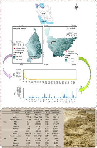
Table 1. Geographical locations and characteristics of stations.

Station	River	Area (km^2)	Latitude (N)	Longitude	Altitude (m)
Sarighamish	ZarrinehRoud	7160	36.48	46.48	1380
Varand	Chahardangeh	1198.3	36.35	53.19	1722.5

As stated above, the area of the Saeenghale sub-basin is 7160 km², which is seven times greater than that of the Sari sub-basin with 1198.3 km². ULB is located in northwestern Iran (44°7′ to 47°53′E and 35°40′ to 38°30′N) with 51,876 km², which amounts to 3.15% of the area of all basins in Iran. ULB consists of 24% land and 11% Urmia Lake. ZarrinehRoud River is one of the biggest rivers in Urmia Lake basin, which debouches to Urmia Lake (24% of the total intake to Urmia Lake). It is 302 km long, with an average annual water flow of 1583 MCM. This river originates in Chehelcheshme Mountains, crosses Shahindezh, Miandoab and Keshavarz cities and finally reaches the southern part of Urmia Lake. Based on the literature, the flow rate of ZarrinehRoud River varies from 120 to 10 m³/s annually. This significant fluctuation in river flow rate depends on climatic conditions. There are also dissolved components in ZarrinehRoud River that lead to dissolved sediment loads. These data are measured by hydrological experts in Urmia environmental and water organizations. Sarighamish is a hydrometric station located on this river. This station is located in the Saeenghale sub-basin of ULB (Emdadi et al., 2016; Ghavidel & Montaseri, 2014). Sari City is the capital city of Mazandaran, Iran, which is located at 36° 34′ 4^″N, 53° 3′ 31^″E. Based on the literature, the climate of this city is mild, with much rain in winter (Vatanpour et al., 2020). The annual average temperature is reported to be 16.7°C. Moreover, on average, the month with the highest temperature is August at 25.2°C and February is defined as the coldest month with a temperature of 25.2°C. Additionally, the average precipitation of Sari City is 690 mm per year (Ghanbarpour et al., 2013). The lowest rainfall occurs in June (23 mm), while the highest rainfall (98 mm) occurs in December. Tajan River is known as the most important river of Sari City since it provides water supply to the whole watershed. Chahardangeh River is one of the principal tributaries of Tajan River, which initiates in Kiyasar region mountains. Chahardangeh River, of total length 95.73 km, is located in the Sari sub-basin of Mazandaran province with an area of 1198 km². Moreover, Sari sub-basin is located between (86° 46′ 38.8^″ to 30° 55′ 19. 2^″N) and (52° 46′ 44.8^″ to 6° 56′ 30.1^″E); it also has some hydrometric stations. Hydrometric data from Varand Station on Chahardangeh River from July 1995 to August 2017 are employed in this study.

In the present study, for modeling discharge and SSL data, all data series are divided into two categories, namely 75% and 25% of the entire data series for training and testing, respectively. From Sarighamish Station, data for 15 years (0.75 × 244 = 184) are for training, and data for the remaining five years (0.25 × 244 = 61) are considered for testing. From Varand Station, data for 17 years (0.75 × 262 = 197) are for training, and data for the remaining six years (0.25 × 262 = 65) are for testing. Additionally, input data for modeling in this study are SSL and discharge data from the selected stations.

3. Methodology

3.1. Sediment rating curve (SRC)

The SRC is a mathematical equation relating water discharge and sediment concentration. The SRC is an essential tool when there is no manpower, regular sediment sampling or laboratory investigation. The SRC can be displayed as either an equation or a graph, relating sediment and discharge, which help to solve sediment related problems efficiently. SRC equations and curves are mainly used in sediment transport estimation in rivers (Demirci & Baltaci, 2013). The SRC often comes in the form of power equation (Kisi & Zounemat-Kermani, 2016). Additionally, a rating curve can help experts to estimate sediment loads using streamflow data. Equation (1) demonstrates the equation in detail, which is basically an exponential regression between SSL and discharge: (1) $\text{SSL}=\text{a}{Q}^b$(1) in which Q stands for discharge (m³/s), SSL denotes suspended sediment load (mg/L) and a and b are constant coefficients.

3.2. Intrinsic time-scale decomposition (ITD)

ITD, a time–frequency analysis method, was first presented by Frei & Osorio (2007). ITD has the ability to decompose complex, nonlinear and non-stationary signals into a group of PRCs with few iterations. The principal purpose of ITD is to assimilate higher signals into several PRCs. ITD is developed with the following steps: (2) $x\left(t\right)=Hx\left(t\right)+L\left(t\right)=\left(1-L\right)x\left(t\right)$(2) The operator L is considered to represent local extrema of X_t, which removes the baseline signal. The performance of the operator results in precise rotation. PRCs can be computed by $Hx(t)=(1-L)x(t).$ Furthermore, it is decomposed into signals of $x(t)$. We consider H(t) like $Hx(t)$ and L(t) like $x(t)=Lx(t)$, i.e. the mean of signals.

The steps of ITD algorithms include the following.

1. Defining the extreme points of x(t) as an input signal with the occurrence time of τ_k, where k = 0, 1, 2, … with τ₀ = 0 as the first signal

2. Defining x(t), L(t) and H(t) as input signal and operators on the interval [0, τ_k + 2], respectively. It is noteworthy that operator L is considered to be a linear function on the interval [τ_k, τ_k + 1] during the baseline extraction process. The baseline extraction operator is computed as follows: (3) $\begin{array}{rl}Lx(t)& =L(t)=L_k+\left(\frac{L_{k+1}-L_k}{x_{k+1}-x_k}\right)(x(t)-x_k),\\ & t\in ({\tau }_k,{\tau }_{k+1}),\end{array}$(3) and (4) $\begin{array}{rl}{L}_{k+1}& =\alpha \left[x_k+\frac{({\tau }_{k+1}-{\tau }_k)}{{\tau }_{k+2}-{\tau }_k}(x_{k+1}-x_k)\right]\\ & +(1-\alpha )x_{k+1}\end{array}$(4) in which 0 < α < 1 is taken as a constant parameter (α = 1/2). The process of making monotonic original signal generation x(t) between the extrema points is an essential step in defining PRCs.

3. $H(t)$ can be defined as follows for extracting PRCs: (5) $Hx(t)=(1-L)x(t)=H(t)=x(t)-L(t)$(5)

PRCs can be computed by subtracting the baseline from the input signal.

1. The process is repeated (Equations 9 and 10) until a monotonic function is constructed by baseline (L(t)), which is a single signal divided into PRCs: (6) $x(t)=\sum _{i=1}^p{H}^i(t)+L^p(t)$(6) in which p is the number of PRCs constructed. The critical concepts about the ITD model can be summarized as low computation time, free transient smoothing, smearing in time-scale space solving, iteratively generating optimum PRCs and constant shifting. Additionally, because of feature extraction and filtering, this method can perfectly adapt to real-time data (naturally accrued) while maintaining its initial structure. More details about the ITD method can be found in Frei and Osorio (2007) and Wang et al. (2021).

3.3. Multi-Objective genetic algorithm-based EPR (MOGA-EPR)

EPR is one kind of hybrid and nonlinear regression mathematical method that is hybridized with genetic algorithms (GAs) (Giustolisi & Savic, 2006). In other words, a GA is used for searching for exponents in a symbolic formula based on a regression technique. This method demonstrates the physical polynomial structure of a system. The main objective of polynomial models is to combine output variables with functions. EPR can be summarized in two main steps, namely (a) structure generation made by a GA, and (b) estimating constant variables using the least squares (LS) method. Based on the EPR model, the prevalent mathematical formula is shown as follows: (7) $y=\sum _{i=1}^{m}F(X,f(X),a_i)+a_0$(7) where y is the independent variable (output), a_i are parameters needing to be adjusted, F and f are processes-based user-defined functions, X is an input matrix and m is the number of terms excluding a₀. The input matrix can be defined as (8) $\begin{array}{rl}\mathbf{\text{X}}& =\left[\begin{array}{cccccc}{x}_{11}& x_{12}& x_{13}& \dots & \dots & x_{1k}\\ x_{21}& x_{22}& x_{23}& \dots & \dots & x_{2k}\\ x_{31}& x_{32}& x_{33}& \dots & \dots & x_{3k}\\ \dots & \dots & \dots & \dots & \dots & \dots \\ \dots & \dots & \dots & \dots & \dots & \dots \\ x_{N1}& x_{N2}& x_{N3}& \dots & \dots & x_{NK}\end{array}\right]\\ & =\left[\begin{array}{ccccc}{x}_1& x_2& x_3& \dots & x_{1k}\end{array}\right]\end{array}$(8) It is worth mentioned that the performance of the EPR model has a direct relationship with certain factors, including the number of inputs, selected functions (e.g. logarithmic, hyperbolic, exponential, etc.) (Giustolisi & Savic, 2006). Based on the GA algorithm, a population of solutions as individual chromosomes is generated by the LS method (minimizing the sum of squared errors). Thus, the general EPR equation is expressed as follows: (9) $\begin{array}{rl}\hat{Y}& =a_0+\sum _{j=1}^m{a}_j\cdot (X_i{)}^{ES(j,1)}\cdots (X_k{)}^{ES(j,k)}\\ & \cdot f((X_i{)}^{ES(j,k+1)}\cdots (X_k{)}^{ES(j,2k)}\end{array}$(9) in which m is the maximum number of additive terms, $X_i$ and $\hat{Y}$ are model inputs and outputs, respectively, $f$ and ES are user-defined functions and k is the number of input variables. More details about the EPR method can be found in Bonakdari et al. (2017) and Ghaemi et al. (2021).

3.4. Model tree

The MT method was first introduced by Quinlan (1992). It is a kind of machine learning method that deals with the classification of extensive data and, as a result, generates robust and rigorous models. MT is based on a binary decision tree; thus, it generates tree-based models and is used for continuous class learning. It is noteworthy that decision trees are suitable for categorical type data, but it is applicable for numerical type data too (Quinlan, 1992). It is used to find a proper relationship between input(s) and output variables by utilizing linear regression models to primary leaf nodes (parent nodes).

MT is based on the “divide-and-conquer” method, in which the data sets either connect to a leaf (parent node) or split into subsets in order to evaluate results within the process. In some cases, these divisions result in complex structures; thus, it prunes back by new sub-trees and leaves. Computing the standard deviation (sd) of data sets is the first step in the MT method. The data sets are then split to generate a decision tree. Eliminating over fitted outcomes (pruning) is the second step in the MT method. Pruning techniques, which are based on regression functions, are useful in omitting sub-trees.

The standard deviation (error) is computed as follows: (10) $\mathrm{SDR}=\mathrm{sd}\left(T\right)-\sum \frac{\left|T_i\right|}{\left|T\right|}\mathrm{sd}\left(T_i\right)$(10) in which “sd” signifies the standard deviation, T is a set of examples that reach the primary node and T_i denotes the subset of patterns that possess the ith outcome of the potential data set. By inspecting all outcomes, the MT method selects a node that minimizes the error. The strong points of the MT method include error estimation in unseen cases, utilizing multivariate regression methods in each node, simplification of linear models to minimize error and smoothing predicted values. More information about the MT method can be found in Ghaemi et al. (2019).

3.5. Hybrid ITD decomposition-based models

In nature, hydro-climatic time series often comprise many intrinsic mode functions with different frequencies and exhibit complex nonlinear characteristics. In addition, the results of climate change (such as extreme weather) and human activities (such as environmental pollution and deforestation) are becoming prominent, and these adverse hydrological parameters might lead to deviation from normal climatic patterns and thus accurate prediction could be difficult to achieve. Consequently, the performance of a single prediction model is often not advised if the original signal (or one resolution component) is directly adopted as the input variable.

Signal decomposition algorithms can decompose hydrological time series into a set of relatively stable sub-series and reduce modeling difficulty. Hence, sub-series decomposed by the pre-processing algorithm, ITD, include only a similar scale of hydrological variables and thus are easier to predict. ITD is firstly used to decompose suspended sediment load and river flow time series into a set of sub-series and then a standalone MT and MOGA-EPR are applied to build adequate models for the prediction of each sub-series according to their own characteristics. A schematic diagram of the proposed hybrid ITD-MT and ITD-EPR models is given in Figure 2.

Figure 2. Schematic diagram of hybrid ITD-based–MT/EPR model.

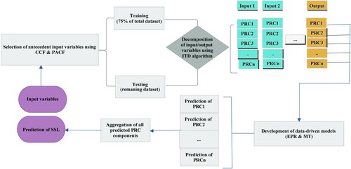
The pre-processing-based models (i.e. ITD-MT and ITD-EPR) comprise the following main steps. In the first step, the original data is divided into two parts, namely the training and testing parts. Secondly, the ITD procedure is employed in order to decompose the original input and output time series E(t) into several PRC components H(t) (i = 1, 2, 3, … , n). In the next step, for each extracted PRC component (for example PRC1), MT and EPR models are established as SSL predicting tools to simulate the decomposed PRC components, and to compute each component by the same sub-series (PRC1) of input variables, respectively. Finally, the predicted values of all extracted PRC components using MT and EPR models are aggregated to generate the SSL, and then the error via the predicted data set is evaluated.

To summarize, hybrid ITD and MT/EPR predictive approaches are employed according to the “decomposition and ensemble” idea. The decomposition is used to simplify the forecasting skill, while the aim of the ensemble is to formulate a consensus prediction on the original data. In this study, for validating and making the pattern of the provided PRC components (e.g. PRC1, PRC2, PRC3) reflect the prediction model and enhancing the SSL prediction accuracy, data sets from Sarighamish and Varand Stations in Iran are selected.

3.6. Statistical performance evaluation measures

In order to determine the best model, five statistical criteria, namely the coefficient of determination (R²), the root mean square error (RMSE), Legates–McCabe’s Index (LMI), the ratio of RMSE to standard deviation (RSD), Willmott’s index of agreement (WI) and the Akaike information criterion (AIC) are implemented as shown in Equations (11) to (15) (Moeeni et al., 2017; Sun et al., 2021; Zeynoddin et al., 2019): (11) $\begin{array}{rl}{R}^2& ={\left(\frac{\sum _{i=1}^N(\text{SS}{\text{L}}_o-\overline{\text{SS}{\text{L}}_o})(\text{SS}{\text{L}}_m-\overline{\text{SS}{\text{L}}_m})}{\sqrt{\begin{array}{c}\sum _{i=1}^N{({SSL}_o-\overline{\text{SS}{\text{L}}_o})}^2\\ \sum _{i=1}^N{(\text{SS}{\text{L}}_m-\overline{\text{SS}{\text{L}}_m})}^2\end{array}}}\right)}^2,\\ & \text{ideal}\text{value}=1\end{array}$(11) (12) $\begin{array}{rl}\text{RMSE}& =\sqrt{\frac{1}{N}\sum _{i=1}^N{(\text{SS}{\text{L}}_m-\text{SS}{\text{L}}_o)}^2},\text{ideal}\text{value}=0\end{array}$(12) (13) $\begin{array}{rl}\text{LMI}& =1-\left[\frac{\sum _{i=1}^N|\text{SS}{\text{L}}_o-\text{SS}{\text{L}}_m|}{\sum _{i=1}^N|\text{SS}{\text{L}}_o-\overline{\text{SS}{\text{L}}_o}|}\right],\text{ideal}\text{value}=0\end{array}$(13) (14) $\begin{array}{rl}\text{RSD}& =\frac{\text{RMSE}}{\text{STDE}{\text{V}}_{\text{obs}}},\text{ideal}\text{value}=0\end{array}$(14) (15) $\begin{array}{rl}\text{WI}& =1-\left[\frac{\sum _{i=1}^N{(\text{SS}{\text{L}}_0-\text{SS}{\text{L}}_m)}^2}{\begin{array}{c}\sum _{i=1}^N(|\text{SS}{\text{L}}_m-\overline{\text{SS}{\text{L}}_o}|\\ +|\text{SS}{\text{L}}_o-\overline{\text{SS}{\text{L}}_o}|{)}^2\end{array}}\right],\\ & \text{ideal}\text{value}=1\end{array}$(15) (16) $\begin{array}{rl}\text{AIC}& =N\ln (\text{MSE})+2K,\text{ideal}\text{value}\\ & =\text{minimum}\text{value}\end{array}$(16) where $\text{SS}{\text{L}}_o$ and $\text{SS}{\text{L}}_m$ are the observed and modeled values of $\text{SSL}$, respectively. Moreover, $\overline{\text{SS}{\text{L}}_o}$ and $\overline{\text{SS}{\text{L}}_m}$ denote average values of the observed and modeled $\text{SSL}$ data, respectively, N is the total number of data points and K indicates the number of parameters.

4. Results and discussion

The main aim of this study is to evaluate the accuracy of ITD-EPR/MT in predicting SSL at Sarighamish and Varand Stations. Thus, in this section, the performance of the models with different input combinations (some at different lag times) for SSL prediction is investigated. In the present study, for modeling the discharge and SSL data, all data series are divided into two categories, namely 75% for the training and 25% for the testing stages. For instance, for Sarighamish Station, 15 years of data (0.75 × 244 = 184) are for training, and the remaining five years of data (0.25 × 244 = 61) are for testing. For Varand Station, 17 years of data (0.75 × 262 = 197) are for training, and the remaining six years of data (0.25 × 262 = 65) are for testing. After that, the performance of standalone models of EPR and MT, and integrating them with ITD pre-processing, are investigated using some evaluation benchmarks (namely R², RMSE, WI, LMI, RSD and AIC) in the training and testing stages at the two proposed stations.

4.1. Optimum input variable selection for SSL prediction

In this study, the proposed prediction models are developed in a MATLAB^® environment. One of the most remarkable steps in the development of model architectures is to determine the best input variable for modeling. The original (non-ITD) dataset with its statistically substantial lagged variables, determined by cross-correlation functions (CCFs) and partial autocorrelation functions (PACFs) operating in a 95% confidence interval, are applied as inputs for developing the models.

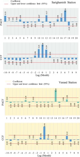
For the time-series datasets of this present study, the time delays of input/output parameters (SSL and Q) are computed by the above-mentioned function. PACF and Partial CCF diagrams of Sarighamish and Varand Stations are shown in Figure 3, in which the vertical axis indicates the time delay (lag number) and the horizontal axis shows the PACF and CCF. Time delays applied to the models are marked in all diagrams. According to Figure 3, two lags of Q are important for modeling SSL at Sarighamish Station. Moreover, PACF is applied for lag time selection of the output variable (SSL). Clearly, the PACF value for Sarighamish Station equals two, whereas no time lag is determined for either the input or output variables at Varand Station.

Figure 3. Partial autocorrelation function (PACF) and cross-correlation function (CCF) between SSL and river discharge for Sarighamish and Varand Stations.

After having considered special input variables for the proposed stations, the best models standing at an acceptable level of accuracy returned by EPR for Sarighamish and Varand Stations are expressed, respectively, as follows: (17) $\begin{array}{rl}\mathrm{SSL}\left(\mathrm{Sarighamish}\right)& =20.1805Q^2\left({\mathrm{SSL}}_{\left(t-2\right)}\right)\\ & \times \exp (0.5Q_1-2Q\\ & -2{\mathrm{SSL}}_{\left(t-2\right)}-2{\mathrm{SSL}}_{\left(t-1\right)})\\ & +53.0092Q_{\left(t-1\right)}^{0.5}{\mathrm{QSSL}}_{\left(t-1\right)}^{1.5}\\ & \times \text{exp}(-2Q_{\left(t-1\right)}-1Q\\ & -1.5{\mathrm{SSL}}_{\left(t-2\right)}-1.5{\mathrm{SSL}}_{\left(t-1\right)})\end{array}$(17) (18) $\begin{array}{rl}\text{SSL}(\text{Varand})& =2.1013Q\text{SS}{\text{L}}_{(t-1)}\\ & \times \exp (-2Q-2\text{SS}{\text{L}}_{(t-1)})\\ & +1.0409Q^2\exp (-2Q-2\text{SS}{L}_{(t-1)})\\ & +0.30265Q^2\text{exp}(Q-2\text{SS}{\text{L}}_{(t-1)})\end{array}$(18)

4.2. Prediction results at Sarighamish Station

As seen in Table 2, the integration of ITD-EPR/MT gives preferable accuracy (i.e. generally the largest R² and the lowest RMSE) compared with the other standalone models, which indicates that intrinsic time-scale decomposition has a high influence in increasing the accuracy of DDM models at Sarighamish and Varand Stations. On the other hand, regarding the performance comparison of the proposed methods at the training stage, it is obvious that, for SSL forecasting, the best predicted SSL values (based on the observed values) are yielded by ITD-EPR with statistical parameters (highest R² = 0.95, lowest RMSE = 1385.4 and RSD = 0.257) compared with inferior results for ITD-MT (R² = 0.93, RMSE = 1537.1 and RSD = 0.285), and standalone models such as EPR (R² = 0.82, lowest RMSE = 2293.7 and RSD = 0.426).

Table 2. Performances of the proposed hybrid and standalone models at Sarighamish Station in training and testing stages.

		R^2	RMSE (ton/day)	WI	LMI	RSD	AIC
Performance metrics—training	EPR	0.82	2293.7	0.93	0.70	0.426	2855.555
	MT	0.81	2882.3	0.88	0.63	0.532	2939.615
	SRC	0.49	4618.3	0.48	0.44	0.857	3107.104
	ITD-EPR	0.95	1385.4	0.97	0.79	0.257	2670.01
	ITD-MT	0.93	1537.1	0.97	0.77	0.285	2708.256
Performance metrics—testing	EPR	0.91	431.06	0.94	0.44	0.55	748.082
	MT	0.73	461.51	0.91	0.37	0.56	756.409
	SRC	0.90	419.44	0.94	0.19	0.49	738.748
	ITD-EPR	0.92	291.81	0.96	0.48	0.35	700.484
	ITD-MT	0.79	456.44	0.93	0.32	0.55	755.061

In the testing stage, evaluation metrics in terms of RSD (0.35) and RMSE (291.81) by ITD-EPR outperform those by other methods such as SRC with higher RSD (40%) and RMSE (43.73%), which stands at the second rank. Despite of acceptable performance of ITD-MT for the training dataset, it has lower accuracy than standalone EPR (15.18% of R² and 37.5% of LMI) for estimated SSL values. In addition, ITD-EPR is selected as the most appropriate model based on AIC (700.484) with the lowest error.

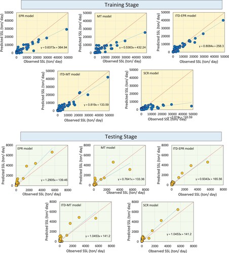
Furthermore, in order to achieve a thorough concept of the efficiency of the proposed models, scatter plots of the observed and estimated values in the training and testing stages are displayed in Figure 4. Scatterplots show a linear regression line (SSL^for = a·SSL ^obs + b, where a is the slope and b is the ordinate intercept) between the measured and estimated values. A greater R² illustrates a better agreement between the observed and forecasted SSL values, and the ITD-EPR model outperforms other methods applied.

Figure 4. Scatterplots of training and testing results by conventional and hybrid models at Sarighamish Station.

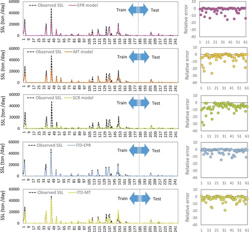
Peak SSL values observed and forecasted by different methods in the training and testing stages are presented in Figure 5. According to Figure 5, among the models, the difference between observed and predicted SSL by the SRC model is the highest. On the contrary, SSL predicted by ITD-EPR (the solid blue line) is the closet to the observed TDS time series (the dotted black line), which explains the best accuracy of this model compared with other models. It is also obvious from Figure 5 that the dispersion of relative errors between the observed and forecasted SSL by the ITD-EPR model is closest to zero.

Figure 5. Comparison of conventional and hybrid models for SSL prediction using time variation graphs at Sarighamish Station.

4.3. Prediction results at Varand Station

Similarly, the evaluation metrics R², RMSE, WI, LMI and RSD applied for SSL prediction at Varand Station for training and testing datasets and results are presented in Table 3. In terms of SSL prediction for the training dataset, integrating ITD and EPR (ITD-EPR) with the lowest error (RSD = 0.35; RMSE = 45.97; WI = 0.96) has significant superiority compared to other models such as ITD-MT (RSD = 0.48; RMSE = 62.48; WI = 0.92), which stands at the second rank, whereas the SRC model (with RSD = 0.67; WI = 0.77; RMSE = 88.62) generates poor performance in SSL estimation (Table 3).

Table 3. Performance of the proposed hybrid and standalone models at Varand Station in the training and testing stages.

		R^2	RMSE (ton/day)	WI	LMI	RSD	AIC
Performance metrics—training	EPR	0.77	65.91	0.91	0.49	0.50	1654.186
	MT	0.69	72.66	0.90	0.51	0.55	1692.602
	SRC	0.70	88.62	0.77	0.52	0.67	1768.837
	ITD-EPR	0.89	45.97	0.96	0.62	0.35	1512.228
	ITD-MT	0.78	62.48	0.92	0.56	0.48	1633.13
Performance metrics—testing	EPR	0.79	231.33	0.86	0.58	0.56	711.6999
	MT	0.69	270.9	0.79	0.50	0.66	732.2275
	SRC	0.79	321.08	0.64	0.48	0.78	752.3197
	ITD-EPR	0.92	168.91	0.93	0.69	0.41	670.8176
	ITD-MT	0.88	195.84	0.91	0.55	0.48	690.0487

Similar to the training stage results, comparison of the proposed models in Table 3 indicates ITD-EPR (RMSE = 168.91; WI = 0.93; LMI = 0.69) and SRC (RMSE = 321.08; WI = 064; LMI = 0.48) attain the highest and lowest SSL forecasting accuracy in the testing stage, respectively. Moreover, an evaluation of the efficiency of ITD in SSL prediction indicates that the integration of this pre-processing method can improve the accuracy of the proposed models. It is shown from Table 3 that, although the MT model estimates SSL values poorly (R² = 0.69 and LMI = 0.5), its integration with the ITD method increases R² and LMI values by roughly 27.53% and 10%, respectively.

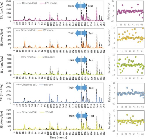
Additionally, scatter plots, relatively error and time series of estimated SSL values versus the observed ones are presented in Figures 6 and 7. In terms of scatter plots, the slope of SSL values for the ITD-EPR model is closest to the ideal line and a number of SSL estimated values are underestimated. Moreover, hybrid models have better performance than other models in estimating peak values. Taking the maximum SSL value as an example (1123.678), the proposed methods, namely EPR, MT, SRC, ITD-EPR and ITD-MT, underestimate by about 18.95%, 35.31%, 63.06%, 5.11% and 13.56%, respectively. In the case of the relative error for the testing dataset, the variations of relative error values are between −5 and 5, whereas those for the best standalone model (EPR) are between −8 and 8.

Figure 6. Scatterplots of training and testing results by conventional and hybrid models at Varand Station.

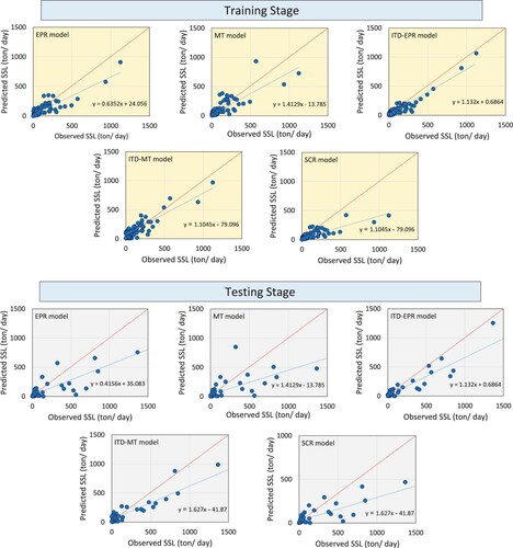
Figure 7. Comparison of conventional and hybrid models for SSL prediction using time variation graphs at Sarighamish Station.

4.4. Discussion and study limitations

The SSL simulations in the present study reveal that there are obvious differences between the original DDMs and data decomposition-based models, indicating the significance of the training framework in prediction models. As stated above, for a standalone prediction model, it is often hard to fully and accurately reflect the formation and changing mechanisms of natural hydrological variables such as SSL since only one resolution component is used for establishing the predicting module. It indicates that other resolution sub-components in the original SSL time series cannot be separated effectively. To avoid this problem, decomposition algorithms are suggested to select various resolution intervals, and after that, the features of each sub-series can be separated. Therefore, the performance of hybrid methods (such as ITD-MT and ITD-EPR) are superior to those of the standard MT and EPR methods, which match the results of recent similar studies (Napolitano et al., 2011; Wu & Huang, 2009).

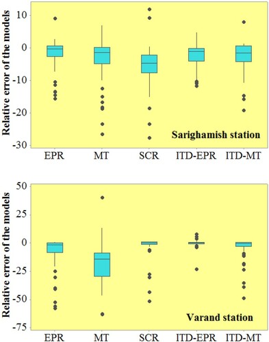
In addition, for further comparison, box plots are employed for evaluating the accuracy of the proposed models in SSL forecasting at two proposed stations. In this study, box plots indicate the spread of relative errors between observed and estimated SSL values based on quartiles so that the whiskers explain the variations outside the 25th and 75th percentiles (Figure 8) (Prasad et al., 2018). Regarding the distribution of the relative errors of the models, the higher and lower capability of ITD-EPR and SRC are clear compared with other approaches. Furthermore, it is obvious that a huge number of SSLs estimated by models are underestimated.

Figure 8. Boxplots of relative predicted error (ton/day) by the hybrid ITD-EPR model compared with the standalone EPR, MT, SCR models and the hybrid ITD-MT model for both tested regions.

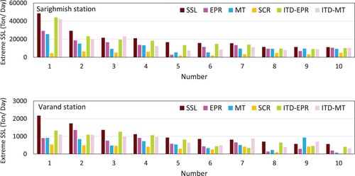
Moreover, the prediction performances of various methods for peak SSL values are compared. The thresholds for sediment series for Sarighamish and Varand Stations are equal to 11164 and 564.721 ton/day, respectively. Therefore, 10 SSL observations are selected exceeding the threshold and their corresponding forecasted values by the proposed models are shown in Figure 9. In case of Sarighamish Station, except the SRC model, which has the lowest accuracy for all maximum SSL values, all other models have approximately the same error for SSL peak values with less than 10,000 ton/day. However, for other peak values, the efficiency of the ITD technique in SSL forecasting is undeniable. The dominant superiority of ITD-EPR in SSL forecasting is summarized with an average error percentage value (13.60%), which is significantly lower than the corresponding ITD-MT (26.79%), EPR (32.26%), MT (41.45%) and SRC (75.56%) for 10 sediment peaks. In the case of Varand Station, all models are roughly incapable of predicting SSL peak values, especially for values greater than 10,000 ton/day. Additionally, ITD-EPR has a good performance in predicting peak values of SSL with an average error percentage value of 25.88% compared to the corresponding ITD-MT (26.52%), EPR (47.51%), MT (45.19%) and SRC (67.16%) values for 10 sediment peak amounts.

Figure 9. Comparison of extreme value predictions of SSL using five conventional and hybrid models at Sarighamish and Varand Stations.

Although the proposed model has an acceptable accuracy in SSL prediction, it is possible to employ other evolutionary DDMs and modern algorithms for integration with pre-processing methods, such as vibrational mode decomposition (VMD) and complete ensemble empirical mode decomposition (CEEMD), to create more accurate models in SSL prediction. With the aim of more accurate SSL estimation, more data samples or different input variables with daily or hourly timescales may be attempted. Consequently, for future work, they may be suggested as the potential measures for improving the accuracy of SSL for forecasting both data samples and different input variables.

5. Conclusions

In this study, the capability of integrating ITD and DDM methods is investigated in SSL forecasting at Sarighamish and Varand Stations in Iran. This study focuses on the effect of the time delay of input/output parameters in SSL predicting. A comparison of result indicates that the ITD data-decomposition method, via decomposing datasets and solving non-stationary behaviors of SSL time-series datasets, has a notable influence on increasing model accuracy. For instance, at Sarighamish Station, the estimated SSL using ITD-EPR has lower errors for RMSE (291.81) and RSD (0.35) compared with other methods. By comparing the performance of EPR and ITD-EPR, it can be seen that the computed value of RMSE decrease from 431.06 to 291.81 and the value of RSD also decreases, from 0.55 to 0.35. At Varand Station, the outcomes demonstrate that EPR and MT are accurate models with the help of the ITD algorithm. However, the results indicate that the MT model attains lower accuracy compared to other DDM models for SSL prediction in terms of R² (0.73) and WI (0.91) at Sarighamish Station and 0.69 and 0.79 at Varand Station, respectively.

Additionally, the proposed models are compared with the sediment rating curve (SRC) empirical method. Outcomes illustrate that SRC provides the greatest average error percentage values for both Sarighamish (75.56%) and Varand (67.16%) Stations compared with those from DDMs.

The application of the decomposition method is thus highly recommended for SSL forecasting with the same scale of input/output variables and watershed properties for evaluating DDM generalization. Although other nonlinear programming simulation methods can be applied to find contributors to SSL in river bodies, it may typically be subjected to a prohibitory computational burden, especially for complex and large river systems estimation.

It should be noted that the selection of the number of training datasets in DDMs has a great impact on the estimation accuracy. It can be expected that the accuracy increases to a remarkable level by increasing the size of the data, since it leads to a better capability of models to predict SSL variability over different periods. The outcomes of this study can assist in obtaining a range of datasets to provide an optimum model for SSL estimation. It appears that the future of SSL prediction by different evolutionary DDMs and creating modern algorithms will be very bright and promising.

Disclosure statement

No potential conflict of interest was reported by the authors.

References

- Adarsh, S., & Reddy, M. J. (2015). Multiscale analysis of suspended sediment concentration data from natural channels using the Hilbert-Huang transform. Aquatic Procedia, 4, 780–788. https://doi.org/https://doi.org/10.1016/j.aqpro.2015.02.097
- Adnan, R. M., Liang, Z., El-Shafie, A., Zounemat-Kermani, M., & Kisi, O. (2019). Prediction of suspended sediment load using data-driven models. Water, 11(10), 2060. https://doi.org/https://doi.org/10.3390/w11102060
- Attar, N. F., Pham, Q. B., Nowbandegani, S. F., Rezaie-Balf, M., Fai, C. M., Ahmed, A. N., ... & El-Shafie, A. (2020). Enhancing the prediction accuracy of data-driven models for monthly streamflow in Urmia Lake basin based upon the autoregressive conditionally heteroskedastic time-series model. Applied Sciences, 10(2), 571. https://doi.org/https://doi.org/10.3390/app10020571
- Alizadeh, M. J., Nodoushan, E. J., Kalarestaghi, N., & Chau, K. W. (2017). Toward multi-day-ahead forecasting of suspended sediment concentration using ensemble models. Environmental Science and Pollution Research, 24(36), 28017–28025. https://doi.org/https://doi.org/10.1007/s11356-017-0405-4
- Bonakdari, H., Ebtehaj, I., & Akhbari, A. (2017). Multi-objective evolutionary polynomial regression-based prediction of energy consumption probing. Water Science and Technology, 75(12), 2791–2799. https://doi.org/https://doi.org/10.2166/wst.2017.158
- Bonakdari, H., Moeeni, H., Ebtehaj, I., Zeynoddin, M., Mahoammadian, A., & Gharabaghi, B. (2019). New insights into soil temperature time series modeling: Linear or nonlinear? Theoretical and Applied Climatology, 135(3), 1157–1177. https://doi.org/https://doi.org/10.1007/s00704-018-2436-2
- Cieśla, M., Gruca-Rokosz, R., & Bartoszek, L. (2020). The connection between a suspended sediments and reservoir siltation: Empirical analysis in the maziarnia reservoir. Poland. Resources, 9(3), 30. https://doi.org/https://doi.org/10.3390/resources9030030
- Coleman, N. L. (1986). Effects of suspended sediment on the open-channel velocity distribution. Water Resources Research, 22(10), 1377–1384. https://doi.org/https://doi.org/10.1029/WR022i010p01377
- Demirci, M., & Baltaci, A. (2013). Prediction of suspended sediment in river using fuzzy logic and multilinear regression approaches. Neural Computing and Applications, 23(1), 145–151. https://doi.org/https://doi.org/10.1007/s00521-012-1280-z
- Ebtehaj, I., Bonakdari, H., & Shamshirband, S. (2016). Extreme learning machine assessment for estimating sediment transport in open channels. Engineering with Computers, 32(4), 691–704. https://doi.org/https://doi.org/10.1007/s00366-016-0446-1
- Ebtehaj, I., Bonakdari, H., Shamshirband, S., & Mohammadi, K. (2016). A combined support vector machine-wavelet transform model for prediction of sediment transport in sewer. Flow Measurement and Instrumentation, 47, 19–27. https://doi.org/https://doi.org/10.1016/j.flowmeasinst.2015.11.002
- Ehteram, M., Ghotbi, S., Kisi, O., Najah Ahmed, A., Hayder, G., Ming Fai, C., … EL-Shafie, A. (2019). Investigation on the potential to integrate different artificial intelligence models with metaheuristic algorithms for improving river suspended sediment predictions. Applied Sciences, 9(19), 4149. https://doi.org/https://doi.org/10.3390/app9194149
- Emdadi, A., Gikas, P., Farazaki, M., & Emami, Y. (2016). Salinity gradient energy potential at the hyper saline Urmia lake–ZarrinehRud river system in Iran. Renewable Energy, 86, 154–162. https://doi.org/https://doi.org/10.1016/j.renene.2015.08.015
- Fard, A. K., & Akbari-Zadeh, M. R. (2014). A hybrid method based on wavelet, ANN and ARIMA model for short-term load forecasting. Journal of Experimental & Theoretical Artificial Intelligence, 26(2), 167–182. https://doi.org/https://doi.org/10.1080/0952813X.2013.813976
- Frei, M. G., & Osorio, I. (2007). Intrinsic time-scale decomposition: Time–frequency–energy analysis and real-time filtering of non-stationary signals. Proceedings of the royal society A: Mathematical. Physical and Engineering Sciences, 463(2078), 321–342. https://doi.org/https://doi.org/10.1098/rspa.2006.1761.
- Ghaemi, A., Rezaie-Balf, M., Adamowski, J., Kisi, O., & Quilty, J. (2019). On the applicability of maximum overlap discrete wavelet transform integrated with MARS and M5 model tree for monthly pan evaporation prediction. Agricultural and Forest Meteorology, 278, 107647. https://doi.org/https://doi.org/10.1016/j.agrformet.2019.107647
- Ghaemi, A., Zhian, T., Pirzadeh, B., Monfared, S. H., & Mosavi, A. (2021). Reliability-based design and implementation of crow search algorithm for longitudinal dispersion coefficient estimation in rivers. Environmental Science and Pollution Research, 1–20. https://doi.org/https://doi.org/10.1007/s11356-021-12651-0.
- Ghanbarpour, M. R., Goorzadi, M., & Vahabzade, G. (2013). Spatial variability of heavy metals in surficial sediments: Tajan river watershed, Iran. Sustainability of Water Quality and Ecology, 1, 48–58. https://doi.org/https://doi.org/10.1016/j.swaqe.2014.04.002
- Ghavidel, S. Z. Z., & Montaseri, M. (2014). Application of different data-driven methods for the prediction of total dissolved solids in the zarinehroud basin. Stochastic Environmental Research and Risk Assessment, 28(8), 2101–2118. https://doi.org/https://doi.org/10.1007/s00477-014-0899-y
- Giustolisi, O., & Savic, D. A. (2006). A symbolic data-driven technique based on evolutionary polynomial regression. Journal of Hydroinformatics, 8(3), 207–222. https://doi.org/https://doi.org/10.2166/hydro.2006.020b
- Hassanpour, F., Sharifazari, S., Ahmadaali, K., Mohammadi, S., & Sheikhalipour, Z. (2019). Development of the FCM-SVR hybrid model for estimating the suspended sediment load. KSCE Journal of Civil Engineering, 23(6), 2514–2523. https://doi.org/https://doi.org/10.1007/s12205-019-1693-7
- Huang, C. C., Fang, H. T., Ho, H. C., & Jhong, B. C. (2019). Interdisciplinary application of numerical and machine-learning-based models to predict half-hourly suspended sediment concentrations during typhoons. Journal of Hydrology, 573, 661–675. https://doi.org/https://doi.org/10.1016/j.jhydrol.2019.04.001
- Jaiyeola, A. T., & Adeyemo, J. (2019). Performance comparison between genetic programming and sediment rating curve for suspended sediment prediction. African Journal of Science, Technology, Innovation and Development, 11(7), 843–859. https://doi.org/https://doi.org/10.1080/20421338.2019.1587908
- Khan, M. Y. A., Tian, F., Hasan, F., & Chakrapani, G. J. (2019). Artificial neural network simulation for prediction of suspended sediment concentration in the river ramganga, Ganges basin, India. International Journal of Sediment Research, 34(2), 95–107. https://doi.org/https://doi.org/10.1016/j.ijsrc.2018.09.001
- Khozani, Z. S., Safari, M. J. S., Mehr, A. D., & Mohtar, W. H. M. W. (2020). An ensemble genetic programming approach to develop incipient sediment motion models in rectangular channels. Journal of Hydrology, 584, 124753. https://doi.org/https://doi.org/10.1016/j.jhydrol.2020.124753
- Kisi, O., & Ozkan, C. (2017). A new approach for modeling sediment-discharge relationship: Local weighted linear regression. Water Resources Management, 31(1), 1–23. https://doi.org/https://doi.org/10.1007/s11269-016-1481-9
- Kisi, O., & Yaseen, Z. M. (2019). The potential of hybrid evolutionary fuzzy intelligence model for suspended sediment concentration prediction. Catena, 174, 11–23. https://doi.org/https://doi.org/10.1016/j.catena.2018.10.047
- Kisi, O., & Zounemat-Kermani, M. (2016). Suspended sediment modeling using neuro-fuzzy embedded fuzzy c-means clustering technique. Water Resources Management, 30(11), 3979–3994. https://doi.org/https://doi.org/10.1007/s11269-016-1405-8
- Kuai, K. Z., & Tsai, C. W. (2012). Identification of varying time scales in sediment transport using the hilbert–Huang transform method. Journal of Hydrology, 420, 245–254. https://doi.org/https://doi.org/10.1016/j.jhydrol.2011.12.007
- Kumar, A., Kumar, P., & Singh, V. K. (2019). Evaluating different machine learning models for runoff and suspended sediment simulation. Water Resources Management, 33(3), 1217–1231. https://doi.org/https://doi.org/10.1007/s11269-018-2178-z
- Liu, Q. J., Zhang, H. Y., Gao, K. T., Xu, B., Wu, J. Z., & Fang, N. F. (2019). Time-frequency analysis and simulation of the watershed suspended sediment concentration based on the Hilbert-Huang transform (HHT) and artificial neural network (ANN) methods: A case study in the loess plateau of China. Catena, 179, 107–118. https://doi.org/https://doi.org/10.1016/j.catena.2019.03.042
- Loska, K., & Wiechuła, D. (2003). Application of principal component analysis for the estimation of source of heavy metal contamination in surface sediments from the rybnik reservoir. Chemosphere, 51(8), 723–733. https://doi.org/https://doi.org/10.1016/S0045-6535(03)00187-5
- Martins, P. D., & Poleto, C. (2017). Principle of maximum entropy in the estimation of suspended sediment concentration. RBRH, 22(0). https://doi.org/https://doi.org/10.1590/2318-0331.011716058
- Meshram, S. G., Singh, V. P., Kisi, O., Karimi, V., & Meshram, C. (2020). Application of artificial neural networks, support vector machine and multiple model-ANN to sediment yield prediction. Water Resources Management, 34(15), 4561–4575. https://doi.org/https://doi.org/10.1007/s11269-020-02672-8
- Mirbagheri, S. A., Nourani, V., Rajaee, T., & Alikhani, A. (2010). Neuro-fuzzy models employing wavelet analysis for suspended sediment concentration prediction in rivers. Hydrological Sciences Journal–Journal des Sciences Hydrologiques, 55(7), 1175–1189. https://doi.org/https://doi.org/10.1080/02626667.2010.508871
- Moeeni, H., Bonakdari, H., & Ebtehaj, I. (2017). Integrated SARIMA with neuro-fuzzy systems and neural networks for monthly inflow prediction. Water Resources Management, 31(7). https://doi.org/https://doi.org/10.1007/s11269-017-1632-7
- Napolitano, G., Serinaldi, F., & See, L. (2011). Impact of EMD decomposition and random initialisation of weights in ANN hindcasting of daily stream flow series: An empirical examination. Journal of Hydrology, 406(3-4), 199–214. https://doi.org/https://doi.org/10.1016/j.jhydrol.2011.06.015
- Nourani, V., Baghanam, A. H., Adamowski, J., & Kisi, O. (2014). Applications of hybrid wavelet–artificial intelligence models in hydrology: A review. Journal of Hydrology, 514, 358–377. https://doi.org/https://doi.org/10.1016/j.jhydrol.2014.03.057
- Nourani, V., Molajou, A., Tajbakhsh, A. D., & Najafi, H. (2019). A wavelet based data mining technique for suspended sediment load modeling. Water Resources Management, 33(5), 1769–1784. https://doi.org/https://doi.org/10.1007/s11269-019-02216-9
- Peterson, K. T., Sagan, V., Sidike, P., Cox, A. L., & Martinez, M. (2018). Suspended sediment concentration estimation from landsat imagery along the lower Missouri and middle Mississippi rivers using an extreme learning machine. Remote Sensing, 10(10), 1503. https://doi.org/https://doi.org/10.3390/rs10101503
- Prasad, R., Deo, R. C., Li, Y., & Maraseni, T. (2018). Ensemble committee-based data intelligent approach for generating soil moisture forecasts with multivariate hydro-meteorological predictors. Soil and Tillage Research, 181, 63–81. https://doi.org/https://doi.org/10.1016/j.still.2018.03.021
- Quinlan, J. R. (1992, November). Learning with continuous classes. In 5th Australian Joint Conference on Artificial Intelligence, Vol. 92, 343–348. https://doi.org/https://doi.org/10.1142/9789814536271.
- Rahgoshay, M., Feiznia, S., Arian, M., & Hashemi, S. A. A. (2019). Simulation of daily suspended sediment load using an improved model of support vector machine and genetic algorithms and particle swarm. Arabian Journal of Geosciences, 12(9), 1–14. https://doi.org/https://doi.org/10.1007/s12517-019-4444-7
- Rajaee, T. (2011). Wavelet and ANN combination model for prediction of daily suspended sediment load in rivers. Science of the Total Environment, 409(15), 2917–2928. https://doi.org/https://doi.org/10.1016/j.scitotenv.2010.11.028
- Rezaie-Balf, M., Kim, S., Fallah, H., & Alaghmand, S. (2019). Daily river flow forecasting using ensemble empirical mode decomposition based heuristic regression models: Application on the perennial rivers in Iran and South Korea. Journal of Hydrology, 572, 470–485. https://doi.org/https://doi.org/10.1016/j.jhydrol.2019.03.046
- Rocco S, C. M. (2013). Singular spectrum analysis and forecasting of failure time series. Reliability Engineering and System Safety, 114, 126–136. https://doi.org/https://doi.org/10.1016/j.ress.2013.01.007
- Roushangar, K., Aghajani, N., Ghasempour, R., & Alizadeh, F. (2021). The potential of ensemble WT-EEMD-kernel extreme learning machine techniques for prediction suspended sediment concentration in successive points of a river. Journal of Hydroinformatics, 23(3), 655–670. https://doi.org/https://doi.org/10.2166/hydro.2021.146
- Safari, M. J. S., & Mehr, A. D. (2018). Multigene genetic programming for sediment transport modeling in sewers for conditions of non-deposition with a bed deposit. International Journal of Sediment Research, 33(3), 262–270. https://doi.org/https://doi.org/10.1016/j.ijsrc.2018.04.007
- Samet, K., Hoseini, K., Karami, H., & Mohammadi, M. (2019). Comparison between soft computing methods for prediction of sediment load in rivers: Maku dam case study. Iranian Journal of Science and technology. Transactions of Civil Engineering, 43(1), 93–103. https://doi.org/https://doi.org/10.1007/s40996-018-0121-4.
- Sharghi, E., Nourani, V., Najafi, H., & Gokcekus, H. (2019). Conjunction of a newly proposed emotional ANN (EANN) and wavelet transform for suspended sediment load modeling. Water Supply, 19(6), 1726–1734. https://doi.org/https://doi.org/10.2166/ws.2019.044
- Sharghi, E., Nourani, V., Najafi, H., & Soleimani, S. (2019). Wavelet-Exponential smoothing: A New hybrid method for suspended sediment load modeling. Environ. Process, 6(1), 191–218. https://doi.org/https://doi.org/10.1007/s40710-019-00363-0
- Singh, V. P., & Krstanovic, P. F. (1987). A stochastic model for sediment yield using the principle of maximum entropy. Water Resources Research, 23(5), 781–793. https://doi.org/https://doi.org/10.1029/WR023i005p00781
- Sun, K., Rajabtabar, M., Samadi, S., Rezaie-Balf, M., Ghaemi, A., Band, S. S., & Mosavi, A. (2021). An integrated machine learning, noise suppression, and population-based algorithm to improve total dissolved solids prediction. Engineering Applications of Computational Fluid Mechanics, 15(1), 251–271. https://doi.org/https://doi.org/10.1080/19942060.2020.1861987
- Tiwari, M. K., & Chatterjee, C. (2010). Development of an accurate and reliable hourly flood forecasting model using wavelet–bootstrap–ANN (WBANN) hybrid approach. Journal of Hydrology, 394(3-4), 458–470. https://doi.org/https://doi.org/10.1016/j.jhydrol.2010.10.001
- Vatanpour, N., Malvandi, A. M., Talouki, H. H., Gattinoni, P., & Scesi, L. (2020). Impact of rapid urbanization on the surface water’s quality: A long-term environmental and physicochemical investigation of Tajan river, Iran (2007–2017). Environmental Science and Pollution Research, 27(8), 8439–8450. https://doi.org/https://doi.org/10.1007/s11356-019-07477-w
- Wang, M., Rezaie-balf, M., Naganna, S. R., & Yaseen, Z. M. (2021). Sourcing CHIRPS precipitation data for streamflow forecasting using intrinsic time-scale decomposition based machine learning models. Hydrological Sciences Journal. (just-accepted). https://doi.org/https://doi.org/10.1080/02626667.2021.1928138
- Wu, Z., & Huang, N. E. (2009). Ensemble empirical mode decomposition: A noise-assisted data analysis method. Advances in Adaptive Data Analysis, 1(01), 1–41. https://doi.org/https://doi.org/10.1142/S1793536909000047
- Zeng, J. X., Wang, G. F., Zhang, F. Q., & Ye, J. C. (2012). The de-noising algorithm based on intrinsic time-scale decomposition. In Advanced Materials Research (vol. 422, pp. 347–352). Trans Tech Publications Ltd. https://doi.org/https://doi.org/10.4028/www.scientific.net/AMR.422.347.
- Zeng, W., Li, M., Yuan, C., Wang, Q., Liu, F., & Wang, Y. (2020). Identification of epileptic seizures in EEG signals using time-scale decomposition (ITD), discrete wavelet transform (DWT), phase space reconstruction (PSR) and neural networks. Artificial Intelligence Review, 53(4), 3059–3088. https://doi.org/https://doi.org/10.1007/s10462-019-09755-y
- Zeynoddin, M., Bonakdari, H., Ebtehaj, I., Esmaeilbeiki, F., Gharabaghi, B., & Haghi, D. Z. (2019). A reliable linear stochastic daily soil temperature forecast model. Soil and Tillage Research, 189, 73–87. https://doi.org/https://doi.org/10.1016/j.still.2018.12.023
- Zhang, Y., Zhang, C., Liu, X., Wang, W., Han, Y., & Wu, N. (2019, June). Fault diagnosis method of wind turbine bearing based on improved intrinsic time-scale decomposition and spectral kurtosis. In 2019 eleventh international conference on advanced computational intelligence (ICACI) (pp. 29–34). IEEE. doi: https://doi.org/10.1109/ICACI.2019.8778629.
- Zounemat-Kermani, M., Mahdavi-Meymand, A., Alizamir, M., Adarsh, S., & Yaseen, Z. M. (2020). On the complexities of sediment load modeling using integrative machine learning: Application of the great river of Loíza in Puerto Rico. Journal of Hydrology, 585, 124759.7. doi:https://doi.org/10.1016/j.jhydrol.2020.124759