Thermal boundary condition analysis of cooling objects exposed to a free impinging jet using the heatline concept

Abstract

Heat and flow pattern of a vertical free jet impinging on a hot disk were numerically investigated. A cylinder with various thicknesses and materials exposed simultaneously to uniform heat flux on one side and a free impinging jet on the other side is simulated by ANSYS Fluent 19.3. For simulations, the thermal boundary condition on the hot surface might differ due to the nature of the heat flow. The Volume of Fluid (VOF) approach is used to model the free jet heat transfer and fluid dynamics with the presence of air, while only the energy equation is solved in the cylinder. Heatline equation is solved to reveal the heat flow direction and effects of different geometry conditions. The maximum heat flux of 2.5 MW/m2 was obtained at the edge of stagnation region for hot target made of copper, while the value was 1.5 MW/m2 when the material was combined with stainless steel. However, the general thermal and hydrodynamic features of the jet flow were not influenced. It means that hot object condition may only affect the balance between heat flux and temperature, and the ideal uniform heat flux on the impinging wall may not be achieved in any experimental conditions.

KEYWORDS:

• Free impinging jet
• cooling
• thermal boundary condition
• Ansys Fluent
• heatline
• nanofluid

Introduction

Heat harvesting from hot objects is a common activity in many industries, from heat exchangers to power plants (Kröger, 2004; Mahdavi et al., 2017; Mahdavi et al., 2015; Mahdavi et al., 2016; Mahdavi et al., 2018a, Mahdavi et al., 2018b; Omidi et al., 2017).A free impinging water jet is often used on hot surfaces with many different shapes, from circular to flat rectangular surfaces (Oztop et al., 2011; Pachpute & Premachandran, 2020; Wu et al., 2019). Liquid is injected from the inlet of a small nozzle with high velocity and impinges on the hot object. The jet flow starts to create a thin layer of liquid just after the stagnation region because of the air–liquid surface tension. As the flow spreads on the hot surface, the velocity decreases as a result of flow resistance and boundary layer formation on the solid wall. This thin liquid layer absorbs the heat and conveys it to the outer region.

Cooling methods using a flow jet depend on the type of heat transfer and limitations, and vary from gases such as air to liquids such as water and nanofluids, both experimentally and numerically (Afroz & Sharif, 2018; Debnath et al., 2020; Du et al., 2020; Hatami et al., 2018; Kim et al., 2019; Nessab et al., 2019; Peng et al., 2020; Wae-hayee et al., 2019; C. Wang et al., 2019; X. L. Yang et al., 2020; Yeranee et al., 2020). Hatami et al. (2018) conducted a two-dimensional (2D) computational fluid dynamics (CFD) simulation of air-jet flow using two different turbulence models. The geometry consisted of a moving diaphragm pushing flow into an orifice and cooling down the hot circular disk at a distance from the orifice outlet. The hot disk was assumed to have a uniform constant temperature with no actual thickness in the modeling. Hatami et al. (2018) used only a quarter of the model (90°) to reduce the expensive computational cost. They investigated the heat transfer improvement and simulation approaches by comparing the results of different turbulent models. However, the thermal boundary conditions, especially how a uniform constant temperature can be obtained in reality considering the flow pattern on the hot target, were not discussed. Moreover, they showed that heat transfer can be improved by nearly 30% in an unconfined test case compared to a confined one, as well as the major impact of dimensionless length on achieving maximum heat transfer.

Air jets were also employed in the experimental work of Kim et al. (2019) and C. Wang et al. (2019), with uniform constant heat flux as the thermal boundary condition. C. Wang et al. (2019) used a heating foil in direct contact with the injecting jet into the main channel flow to provide uniform constant heat flux, and found that air velocity close to the impingement region was a major contributory factor in heat transfer enhancement. Yeranee et al. (2020) experimentally and numerically investigated the cooling impact of an air jet from a nozzle over a hot plate. Copper bars were used under thin stainless steel foil (0.03 mm thickness as the hot plate) to supply constant heat flux as the thermal boundary condition. The authors assumed that uniform heat flux was achieved during the experiment under the foil. For the numerical part, the thin foil was assumed to be a surface and heat flux was distributed uniformly everywhere. The aspects of this thermal boundary condition were assumed to be correct in the numerical simulation, without any explanation of the details. Considering the complexity of the geometry and flow field, they modeled only a quarter of the model. They found that heat transfer can deteriorate at some specific values of pipe length to nozzle diameter ratio because of the blocking impacts of air circulation. Afroz and Sharif (2018) and X. L. Yang et al. (2020) focused on 2D and axisymmetric models of the computational domain for simplicity. The former researchers used a uniform temperature and the latter used a uniform heat flux thermal boundary condition on the target wall, while neither of these studies specified any geometric shape for the hot surface in terms of thickness or material. Nonetheless, it is noted that the Nusselt number showed an initial increase around the stagnation region and then decreased as the flow left the domain. This means that there is a wide range of heat transfer distribution and Nusselt number from the impingement point to the outflow. One would expect to obtain a wide distribution of temperature and heat flux in the case of uniform heat flux and temperature boundary conditions, respectively.

Using a liquid such as water or a nanofluid has more advantages than air in terms of cooling hot surfaces because of the higher thermal conductivity (Ez Abadi et al., 2020; Ghalandari et al., 2019). Peng et al. (2020) used CFD analysis to find the optimum geometry and number of water jet flows in a microchannel with laminar single-phase fluid. The entire three-dimensional (3D) model was simulated by considering the actual shape of hot wall thickness exposed to uniform heat flux. The values for heat transfer and the pumping power of the flow were reported, but no results regarding the solid geometry or material were discussed. However, they found that using multiple jets can have noticeable effects on heat transfer enhancement compared to a conventional single jet. A 2D channel flow of nanofluid was simulated by injecting a nanofluid jet into the domain in the study by Nessab et al. (2019). A magnetic field was located on both sides of the channel, while the solid walls were under the impact of uniform constant heat flux, with no thickness consideration for the walls. The fluid consisted of liquid and fine particles, and a multiphase mixture model was used to model both the liquid phase and nanoparticles. The flow pattern and vortices in the channel revealed no uniformity or symmetry in the distribution of the temperature and streamlines at the top and bottom parts, or in the flow direction. This is one of the challenges regarding the correctness of assumed uniform heat flux on the walls in numerical simulation. Their results showed that using a smaller opening ratio and higher magnetic number can improve heat transfer considerably.

Owing to the high complexity of free jet cooling, with the presence of two phases and a thin layer of liquid on the hot surface (and, in some cases, with boiling), most of the studies have focused on experimental measurements, and numerical simulations are limited to specific cases (Jing-Zhou et al., 2013; Lallave et al., 2007; Lamraoui et al., 2019; Rehman et al., 2017; Selimefendigil & Öztop, 2017a, 2017b, 2018; Turkyilmazoglu, 2019; Y. T. Yang et al., 2015; Zhang et al., 2019; Zuckerman & Lior, 2006). Rehman et al. (2017) conducted numerical simulations to identify the heat and flow features of nanofluid jet over a hot rectangular body. They modeled the entire domain, including the fluid and the solid copper base exposed to uniform heat flux at the bottom, used as an impingement object with actual experimental thickness. The study investigated the effects of various fluid parameters for different boundary conditions, as well as other geometric parameters such as nozzle-to-target spacing. The k–ε turbulence model was used to simulate the flow regimen in turbulent mode, and the multiphase volume of fluid (VOF) method was used to track the interaction between liquid and air. The same methods and models were used by Y. T. Yang et al. (2015). Only a quarter of the full geometry was simulated, by assuming symmetric boundary conditions on two sides. The geometry was constructed based on the experimental studies in the literature. The hot surface was made of Inconel^® alloy plate with a low thermal conductivity of 10.1 W/m.K and thickness of 0.3 mm. The heater block was located under the Inconel alloy plate. Y. T. Yang et al. (2015) considered this whole set-up in their computational domain and applied uniform heat flux under the heater block.

This extensive literature review shows that the main focus of jet flows has been on thermal flow parameters, such as velocity, temperature and Nusselt number. Two different thermal boundary conditions were investigated by researchers, namely uniform heat flux and temperature. However, in many cases, the actual geometry of the hot surface with complete thickness was not considered in the model. Many authors simply assumed that the thermal conditions were achieved by using highly conductive materials or thin plates. In this study, the geometry from an experimental work was chosen to model the flow section as well as the solid part of the set-up. The goal is to seek the heat flow transfer routes by using the heatline concept in the case of a hot surface with different thicknesses and materials. The correctness of the thermal boundary conditions used in the literature is also discussed.

Configuration details and governing formulas

Geometric details

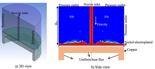
The general configuration of the test case is borrowed from the research provided by Zeitoun and Ali (2012). A free jet of water/nanofluid is vertically released in the gravity direction from a circular nozzle and impinges on a horizontal round disk being heated from the bottom. Instead of using heater bars, as mentioned in the literature review, they used a spiral element heater in direct contact with the bottom of the cylindrical copper disk, and only partially. Also, they added 1 mm of nickel electroplated on top of the copper disk. The details of the exact experimental geometry are shown in Figure 1.

Figure 1. Schematic of the experimental geometry used by Zeitoun and Ali (2012): (a) three-dimensional view; (b) side view.

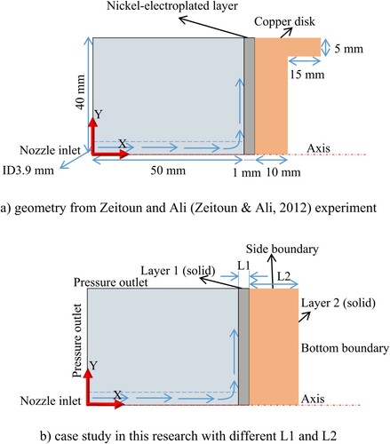
For the purpose of this study, a 2D axisymmetric model is provided to simulate the geometry of Zeitoun and Ali (2012), as well as other changes in the geometry. The axisymmetric model has been repeatedly used by other authors, as explained in the literature review. To emphasize the focus of this study on specific geometries, two main 2D layouts are presented here: one is exactly according to Zeitoun and Ali (2012), shown in Figure 2(a), and the other is similar in the fluid region and slightly different in the solid object, with different thickness and material, as indicated in Figure 2(b). In addition, the flow is highly complex in experimental tests because of turbulence; however, unlike in reality, in simulation the 3D geometry is 100% axisymmetric and turbulent models have to be used (employing average values of variables), so the 3D effects of turbulence will vanish. Therefore, 2D modeling can correctly represent the entire 3D simulation in this case.

Figure 2. Axisymmetric models of the geometries simulated in this study: (a) geometry from Zeitoun and Ali’s (2012) experiment; (b) case study in this research with different L1 and L2.

Heat and multiphase flow equations

Because of the presence of a two-fluid mixture in the domain, the multiphase VOF model (Hirt & Nichols, 1981) was used to solve the interaction between atmospheric air and water. This model is mathematically formulized according to the surface tension and interaction between the phases in each cell.

The mass balance equation is adjusted according to the following assumption: (1) $\left\{\begin{array}{ll}\alpha =1& \mathrm{l}\mathrm{i}\mathrm{q}\mathrm{u}\mathrm{i}\mathrm{d}\\ \alpha =0& \mathrm{a}\mathrm{i}\mathrm{r}\\ 0<\alpha <1& \text{air-liquid-interface}\end{array}\right.$(1) The volume fraction equation in each computational cell is calculated as follows: (2) $\frac{\mathrm{\partial }\left({\alpha }_i{\rho }_i\right)}{\mathrm{\partial }t}+\mathrm{\nabla }.\left({\alpha }_i{\rho }_i\overrightarrow{u}\right)=0$(2) where $\alpha$ and i are the secondary flow volume fraction in the cell and the flow fields, respectively.

The governing equations are followed by: (3) $\begin{array}{rl}& \frac{\mathrm{\partial }\left(\rho \overrightarrow{u}\right)}{\mathrm{\partial }t}+\mathrm{\nabla }.\left(\rho \overrightarrow{u}\overrightarrow{u}\right)=-\mathrm{\nabla }P+\mathrm{\nabla }.\left(\mu \left(\mathrm{\nabla }{\overrightarrow{u}}^T+\mathrm{\nabla }\overrightarrow{u}\right)\right)\\ & \phantom{\frac{\mathrm{\partial }\left(\rho \overrightarrow{u}\right)}{\mathrm{\partial }t}+\mathrm{\nabla }.\left(\rho \overrightarrow{u}\overrightarrow{u}\right)=}+\rho \overrightarrow{g}+\sigma \chi \overrightarrow{\mathrm{\nabla }}\alpha \end{array}$(3) (4) $\begin{array}{rl}& \frac{\mathrm{\partial }\left(\rho E\right)}{\mathrm{\partial }t}+\mathrm{\nabla }.\left(\rho E\overrightarrow{u}\right)=\mathrm{\nabla }.\left(k\mathrm{\nabla }T\right)\end{array}$(4) where E, P and $k$ are the internal energy term, flow pressure and thermal conductivity, respectively. The surface tension term in Equation (3(4) $\begin{array}{rl}& \frac{\mathrm{\partial }\left(\rho E\right)}{\mathrm{\partial }t}+\mathrm{\nabla }.\left(\rho E\overrightarrow{u}\right)=\mathrm{\nabla }.\left(k\mathrm{\nabla }T\right)\end{array}$(4) ) is estimated by using the continuum surface force (CSF) model (Brackbill et al., 1992). The interface curvature $\chi$ is defined based on the surface normal vector $\tilde{n}$: (5) $\chi =-\mathrm{\nabla }.\tilde{n}$(5)

The mass-averaged method is used to obtain the mixture energy term E, represented by $c_{p}T$: (6) $E=\frac{{\sum }_{i=1}^{i=2}{\alpha }_i{\rho }_i{E}_i}{{\sum }_{i=1}^{i=2}{\alpha }_i{\rho }_i}$(6)

The values of the Reynolds number at the exit of the nozzle show the presence of turbulent flow in the domain. Hence, the realizable k–ε model was used to include the effects of turbulence (Bacharoudis et al., 2007; Teodosiu et al., 2014). The differential equations of turbulent kinetic energy ($\kappa$), dissipation rate (ε) and viscosity are defined as follows: (7) $\begin{array}{rl}& \frac{\mathrm{\partial }\left(\rho \kappa u_i\right)}{\mathrm{\partial }{x}_i}=\frac{\mathrm{\partial }}{\mathrm{\partial }{x}_i}\left(\left[\mu +\frac{{\mu }_t}{{\sigma }_k}\right]\frac{\mathrm{\partial }\kappa }{\mathrm{\partial }{x}_i}\right)+G_k+G_b-\rho ϵ\\ & -Y_M+S_k\end{array}$(7) (8) $\begin{array}{rl}& \frac{\mathrm{\partial }\left(\rho ϵu_i\right)}{\mathrm{\partial }{x}_i}=\frac{\mathrm{\partial }}{\mathrm{\partial }{x}_i}\left(\left[\mu +\frac{{\mu }_t}{{\sigma }_{ϵ}}\right]\frac{\mathrm{\partial }ϵ}{\mathrm{\partial }{x}_i}\right)+\rho C_{1}Sϵ\\ & -\rho C_2\frac{{ϵ}^2}{\kappa +\sqrt{ϵ\nu }}+C_{1ϵ}\frac{ϵ}{\kappa }{C}_{3ϵ}{G}_b+S_{ϵ}\end{array}$(8) (9) $\begin{array}{rl}& {\mu }_t=\rho C_{\mu }\frac{{\kappa }^2}{ϵ}\end{array}$(9) (10) $\begin{array}{rl}& C_1=\text{max}\left[0.43,\frac{S\frac{\kappa }{ϵ}}{S\frac{\kappa }{ϵ}+5}\right]\end{array}$(10) (11) $\begin{array}{rl}& C_2=1.9,{\sigma }_{ϵ}=1.2,{\sigma }_k=1.0,C_{1ϵ}=1.44\end{array}$(11) (12) $\begin{array}{rl}& C_{\mu }=\frac{1}{A_0+A_s\frac{\kappa U^{\ast }}{ϵ}}\end{array}$(12)

The definitions of turbulent terms (${\sigma }_k$, $C_2$, ${\sigma }_{ϵ}$, $A_0$ and $C_{1ϵ}$, which are turbulent constants, and ${\mu }_t$, $G_k$, $G_b$, $Y_M$, $S_k$ and $S_{ϵ}$) can be found in Bacharoudis et al. (2007) and Teodosiu et al. (2014).

Grid generation and numerical method

Owing to the simplicity of the 2D geometry, a fully structured mesh is provided here with a fine grid close to the hot surface in contact with water, as shown in Figure 3. The generated mesh for the geometry of Zeitoun and Ali (2012) is also similar to this figure.

Figure 3. Generated mesh for a case study.

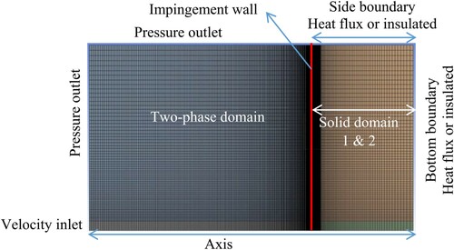
The multiphase VOF model was used to find the interface between air and liquid in the fluid domain from the nozzle inlet to the outside boundary. This was conducted in an implicit unsteady frame, with a time step of 10⁻⁴ s. CSF was used in combination with wall adhesion to model and solve the pressure and interface between the two phases only in computational cells with a volume fraction below 1. The realizable k–ε model was used to model the turbulence in the flow with the scalable wall function to evaluate the viscous sublayer and buffer layer thickness. Because of the convergence issue, a coupled scheme was chosen for the coupling between momentum and energy equations. Only the energy equation was solved in the solid layers. The terms for pressure, momentum, volume fraction, turbulent parameters and energy terms are discretized by the following schemes: PRESTO!, second-order upwind, modified HRIC and second-order upwind, respectively. The mass and heat balance were tracked to ensure that the convergence was obtained in the solution, as well as the temperature on the hot surface and pressure at the nozzle inlet.

Grid study

Owing to the formation of a thin layer of liquid at the vicinity of the wall, it is critical to study the number of generated meshes for the purpose of the grid study. A wide range of meshes was tested, with the main focus on the first layer thickness and the number of cells in the liquid layer. The value of the Nusselt number and deviation from this value were considered as a base for the grid study. The results are presented in Table 1. As can be seen, mesh 3 seems to be the most appropriate grid for this study.

Table 1. Grid study for the case of a water jet with Reynolds number 12,500.

Mesh no.	Total cells	First layer thickness (mm)	No. of layers in liquid phase	Nu	Deviation from experiment
1	8,370	1	1	610.3	−30%
2	17,880	0.1	4	774	−12.6%
3	28,220	0.05	13	839.4	−4.8%
4	43,700	0.02	21	840.7	−4.8%
5	64,410	0.01	32	841.3	−4.7%

Boundary conditions and case studies

Similar boundary conditions were applied in all cases for the flow section of the simulation, as follows: velocity inlet for the nozzle, axisymmetric boundary, pressure outlet for all other flow boundaries, coupled boundary for the hot wall in touch with water, and volume fraction of 1 and 0 for water at the inlet and all other outlets, respectively. Two different materials can be chosen for solid layers 1 and 2, with thicknesses of L1 and L2. Heat flux can be applied to either the bottom or side boundary of the solid layers, as shown in Figure 2. In this case, the other solid boundary will be assumed to be an insulated wall with zero heat flux. Details of the different types of boundaries are illustrated in Figure 3.

In this study, a few cases are simulated based on different base materials and geometries, according to Table 2. Since this research aims to determine the impacts of hot object conditions on the heat transfer, the cases in Table 2 are compared under similar values of flow and heat condition.

Table 2. Conditions of the simulation case studies.

Case no.	Geometry	L1 (mm)	L2 (mm)	Bottom boundary heat (W)	Side boundary heat (W)	Solid layer 1 material	Solid layer 2 material
1	Figure 2(a)	1	10	503	0.0	Nickel	Copper
2	Figure 2(b)	1	10	503	0.0	Nickel	Copper
3	Figure 2(b)	50	0.0	503	0.0	–	Copper
4	Figure 2(b)	50	0.0	0.0	503	–	Copper
5	Figure 2(b)	50	0.0	503	0.0	–	Nickel
6	Figure 2(b)	3	50	503	0.0	Stainless steel	Copper

Results and discussion

As the first step, the results of numerical models are compared with available experimental measurements in the literature. Hence, the findings of the study by Zeitoun and Ali (2012) are borrowed to confirm the validity of the current method. Since Zeitoun and Ali focused on water and nanofluid jets in their work, the validation is provided here for both water and nanofluid according to the following mixture properties for nanofluid: (13) $\begin{array}{rl}& {\rho }_{nf}=\frac{\sum {\phi }_k{\rho }_k}{\left(1-\phi \right)+8\phi {\left(\frac{d_p}{2}+t_v\right)}^3/d_p^3}\end{array}$(13) (14) $\begin{array}{rl}& t_v=-0.0002833{\left(\frac{d_p}{2}\right)}^2+\frac{0.0475d_p}{2}-0.1417\end{array}$(14) (15) $\begin{array}{rl}& c_{p_{nf}}=\frac{\sum {\phi }_k{\rho }_k{c}_{p_k}}{{\rho }_{nf}}\end{array}$(15) (16) $\begin{array}{rl}& \frac{k_{nf}}{k_w}=1+4.4R{e}_B^{0.4}P{r}^{0.66}{\left(\frac{T}{T_{ref}}\right)}^{10}\left(\frac{k_p}{k_w}\right){\phi }^{0.66}\end{array}$(16) (17) $\begin{array}{rl}& R{e}_B=\frac{{\rho }_w{u}_B{d}_p}{{\mu }_w}\end{array}$(17) (18) $\begin{array}{rl}& u_B=\frac{2K_B}{\pi {\mu }_w{d}_p^2}\end{array}$(18) (19) $\begin{array}{rl}& \frac{{\mu }_{nf}}{{\mu }_w}=\frac{1}{1-34.87{\left(d_p/d_c\right)}^{-0.3}{\phi }^{1.03}}\end{array}$(19) where $\phi$, nf and w represent the nanofluid volume fraction, nanofluid and water, respectively. Density is borrowed from Sharifpur’s model (Sharifpur et al., 2016) and other properties are taken from Corcione (2011). Because of the impact of nanoparticles on the surface tension of water, the new surface tension of the nanofluid can be defined as (Meissner & Michaels, 1949): (20) $\begin{array}{rl}\frac{{\sigma }_{w-air}-{\sigma }_{nf-air}}{{\sigma }_{w-air}}& =-7.773\times {10}^{-3}\text{ln}\\ & \times \left(\frac{\phi }{7.673\times {10}^{-7}}+1\right)\end{array}$(20)

The surface tension correlation was implemented into the program for simulation. The properties of nanoparticles and other solid materials are presented in Table 3.

Table 3. Solid and nanoparticle properties.

Material	$\rho$ [kg/m^3]	$c_p$ [J/kg.K]	$k$ [W/m.K]
Alumina nanoparticles	3900	760	39
Copper	8900	381	388
Nickel	8900	460	91
Stainless steel 304	8000	500	16

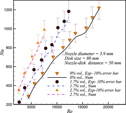
The other useful parameters are presented here: (21) $\begin{array}{rl}Re& =\frac{\rho u_{ip}{D}_{ip}}{\mu },D_{ip}=D_j{\left(\frac{u_j}{u_{ip}}\right)}^{0.5},\\ u_{ip}& =\sqrt{u_j^2+2g{H}_D}\end{array}$(21) (22) $\begin{array}{rl}Nu& =\frac{hD}{k},h=\frac{q}{\left(T_s-T_j\right)}\end{array}$(22) where s, j and ip refer to the disk surface, jet at the nozzle and impingement point, respectively. D is the disk diameter and H is the nozzle to disk spacing. The outlet of the nozzle is circular, with a diameter of 0.0039 m. The space to target distance is 0.05 m and the hot disk diameter is 0.08 m. The range of Reynolds number is from 4000 to 18,000, which can lead to a velocity range of 0.8–4 m/s. The concentration of the nanoparticles at the nozzle exit is assumed to be 1.7%vol and 2.7%vol.

The simulation results are compared to measurements obtained by Zeitoun and Ali (2012) in Figure 4. The error bars are within 10% of the experimental values, which are found to be in good agreement with the numerical results. This proves the ability of the models and the accuracy of the mesh used in the simulations.

Figure 4. Validation study of the numerical model in this research against the experimental work of Zeitoun and Ali (2012).

The results of the average Nusselt number for various values of the Reynolds number and different nanofluid concentrations are shown in Figure 5. Since both local heat flux and temperature on the hot plate vary in the radial direction, the integral form of the heat transfer coefficient has to be used as a user-defined function in CFD tools, according to the following formula: (23) $Nu=\frac{D}{k}\left[\frac{1}{A}\underset{A}{\overset{}{\int }}\frac{q_{cell}}{\left(T_{cell}-T_j\right)}dA\right]$(23) where the term in the bracket is the average heat transfer coefficient on the hot plate. 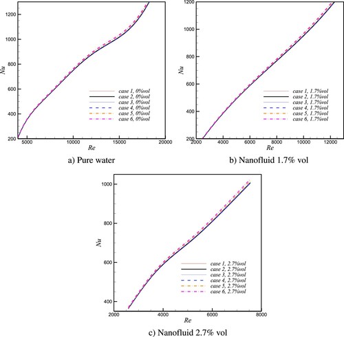$q_{cell}$ and $T_{cell}$ are, respectively, the local heat flux value and temperature on the hot plate according to the corresponding computational cell. The results of the average Nusselt number for different cases are presented in Figure 5. It is observed that in spite of changing the geometry and material, the average Nusselt number is barely affected in either pure water or nanofluid at different volume fractions. This may be caused by the fact that heat flux and temperature can interact in such a way that the energy transfer has to be conserved, and consequently the average values of heat transfer features are only slightly influenced.

Figure 5. Nusselt number vs Reynolds number for the different cases.

The results of heat flux distribution on the hot impinging wall are shown in Figure 6 for various cases. The heat flux is distributed according to the strength of the flow on the surface. In other words, the jet flow experiences its maximum strength in the first impinging area, meaning the stagnation region. Then, as the boundary layer is formed, harvesting of heat transfer is reduced in the direction of the flow on the surface after the stagnation region. It can also be clearly observed that the smallest change in the material and thickness of the base plate can drastically affect the heat flux distribution. The highest range of distribution is found in case 3, where there is one layer of copper with 50 mm thickness. In contrast, as the thermal conductivity of the plate drops considerably in case 6, with one thin layer of stainless steel, the trend changes towards a more uniform heat flux distribution. In addition, the value of maximum heat flux changes from 1.5 to 2.5 MW/m², an increase of almost 40%, from case 6 to case 3.

This uniformity in the heat flux in case 6 can lead to a large spread of temperature on the hot surface, with the maximum temperature at the edge of the surface, as shown in Figure 7. As anticipated, the most uniform temperature distribution is obtained in case 3, with 50 mm of copper plate. Both the heat flux and the temperature prove that cooling of the hot target is highly dependent on material and geometry. For instance, the minimum temperature shows an increase of nearly 14% from case 6 to case 3. However, the local heat transfer coefficient on the hot surface reveals the opposite, as illustrated in Figure 8. Because of the distribution of both heat flux and temperature (with a lack of any conventional thermal boundary condition, such as uniform temperature or heat flux), the heat transfer coefficient was defined based on local values in each computational cell, as follows: (24) $h_y=\frac{q_{cell}}{\left(T_{cell}-T_j\right)}$(24)

Figure 6. Local heat flux on the impinging surface in the radial direction (Y in this study).

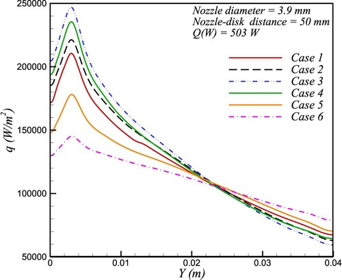
Figure 7. Local temperature on the hot impinging surface in the radial direction (Y in this study).

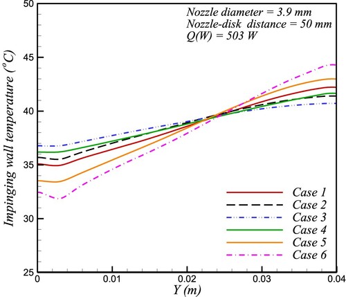
Figure 8. Local heat transfer coefficient on the hot impinging surface in the radial direction (Y in this study).

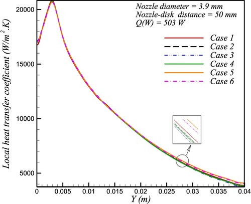
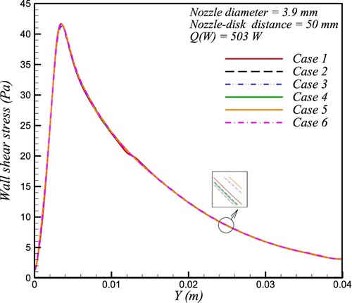
All cases show the same heat transfer coefficient and a similar trend in Figure 8. High heat transfer occurs in the stagnation region, with the maximum value at the edge of this region. Similar behavior is observed for the shear stress distribution in Figure 9. From Figures 8 and 9, it can be concluded that, first, the material and geometry of the heating base plate have no influence on the flow and thermal features of the jet flow on the impinging surface, and secondly, the impact of the jet flow dominates and rules the energy transport in the cooling object. This means that heat transfer occurs in the base plate in such a way that the exchange between heat flux and temperature distribution can be balanced towards reaching the same heat and mass transfer in the jet flow.

Figure 9. Local shear stress over the hot impinging surface in the radial direction (Y in this study).

One useful method in thermal analysis is the concept of the heatline, as developed by Kimura and Bejan (1983). They proposed that energy can be transported on a specific route, similarly to fluid flow. The energy resulting from the temperature difference between two points has to flow from the higher temperature to the lower. The heat cannot cross the heatlines and this can help in tracking the way in which energy is transported. The other main advantage of using heatline is concerned with obtaining specific thermal boundary conditions. For instance, a sharp slope in the heatlines can indicate the presence of a strong temperature gradient on a boundary where obtaining a more uniform temperature distribution is the final goal. The heatline can help the researcher to modify the material, shape and thickness of the section to reach such a goal. This analogy comes from the similarity between a stream function definition and energy balance terms, rearranged as follows.

Continuity equation in axisymmetric flow and stream function: (25) $\begin{array}{rl}& \frac{1}{r}\frac{\mathrm{\partial }\left(r{u}_r\right)}{\mathrm{\partial }r}+\frac{\mathrm{\partial }\left(u_x\right)}{\mathrm{\partial }x}=0\end{array}$(25) (26) $\begin{array}{rl}& u_r=-\frac{1}{r}\frac{\mathrm{\partial }\left(\psi \right)}{\mathrm{\partial }x},u_x=\frac{1}{r}\frac{\mathrm{\partial }\left(\psi \right)}{\mathrm{\partial }r}\end{array}$(26) Energy equation in axisymmetric flow and heatline: (27) $\begin{array}{rl}& \frac{1}{r}\frac{\mathrm{\partial }}{\mathrm{\partial }r}\left[r\left(\rho c_p{u}_{r}T-k\frac{\mathrm{\partial }T}{\mathrm{\partial }r}\right)\right]+\frac{\mathrm{\partial }}{\mathrm{\partial }x}\left[\rho c_p{u}_{x}T-k\frac{\mathrm{\partial }T}{\mathrm{\partial }x}\right]\\ & =0\end{array}$(27) (28) $\begin{array}{rl}& \frac{\mathrm{\partial }H}{\mathrm{\partial }x}=r\left(\rho c_p{u}_{r}T-k\frac{\mathrm{\partial }T}{\mathrm{\partial }r}\right),\\ & \frac{\mathrm{\partial }H}{\mathrm{\partial }r}=r\left(\rho c_p{u}_{x}T-k\frac{\mathrm{\partial }T}{\mathrm{\partial }x}\right)\end{array}$(28) where r (or Y in this study) represents the radial direction. Since the outcomes of Ansys Fluent are obtained in axisymmetric coordinates, the continuity and energy equations also need to be expressed in this way. The analogy indicated in Equations (25(26) $\begin{array}{rl}& u_r=-\frac{1}{r}\frac{\mathrm{\partial }\left(\psi \right)}{\mathrm{\partial }x},u_x=\frac{1}{r}\frac{\mathrm{\partial }\left(\psi \right)}{\mathrm{\partial }r}\end{array}$(26) )–(28) can indicate the behavior of the energy transport and, more importantly, its direction, since having the values of velocity components (and $u_x$) in each point can give the direction of the flow tangential to the streamline. The same concepts can be used to obtain the energy transport direction. The two terms in Equation (28) represent the axial and radial components of the volumetric energy flux vector. Similarly to the velocity vector and streamline, the energy components in Equation (28) are defined as user functions in Ansys Fluent, and the direction of the vector made by these components leads to energy lines or heatlines.

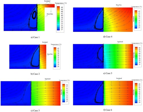
With this method, the heatline and the direction of heat flow are specified, as shown in Figure 10. The heatlines contain constant values of heat, which is only transferred between two lines. In case 1, with actual experimental geometry, and case 2, it is observed that thermal energy is transported from the uniform heat flux boundary with a noticeable slope, to reach the impinging hot wall in contact with the water jet. As a result of the large thermal conductivity of the copper layer in cases 1 and 2, heat directly flows towards the nearest location on the impinging wall with the highest heat transfer coefficient. As the thickness of the copper layer is increased in case 3, with no other layer, a gradual smaller slope is formed for the heat transfer line. By changing the heat flux boundary to the side, the heat travels a long distance from one corner of the side to reach the stagnation region with the highest heat transfer coefficient. It seems that the energy path takes a larger slope towards the hot surface. With the lowering of the solid thermal conductivity in case 5, a more uniform distribution of energy transportation is achieved, and only close to the impinging wall is there a slight slope in the heatline. This is caused by the fact that energy follows the shortest and easiest routes to the heat removal surface, and with the decreasing thermal conductivity and rise in thermal resistance, the easiest route seems to be the shortest with the least slope. Considering all of these observations regarding different materials and thicknesses, an almost uniform heat flux would be expected on the hot surface by combining copper with a thin layer of low thermal conductivity stainless steel, as shown in Figure 10(f). There is a gradual slope in the energy lines in the copper layer, and the curves flatten near the thin stainless steel owing to the high thermal resistance of this layer. The thermal damping impact of stainless steel also increases the temperature everywhere in the copper layer.

Figure 10. Heatline and heat transfer direction shown with temperature contours for both the solid and fluid regions: (a) case 1; (b) case 2; (c) case 3; (d) case 4; (e) case 5; (f) case 6.

Conclusion

The effects of different materials and geometries of a hot object exposed to a free cooling jet were numerically investigated. This study aimed to discuss the challenge of the appropriate definition of thermal boundary conditions for cooling objects, as most researchers tend to simply assume uniform heat flux or temperature boundary conditions, either in experiments or in simulations. The multiphase VOF method combined with the k–ε turbulence model and energy equation were used to solve heat and flow in the fluid and solid domains, respectively. Six cases were modeled for the purposes of this study. Case 1 was based on an experimental geometry in the literature. The initial results of numerical calculations were compared with case 1, and good agreement was found. However, the heat flux distribution on the impinging wall showed a large range from the stagnation region to the edge of the hot surface. This means that the assumption of uniform heat flux on the impinging wall cannot be obtained in the laboratory. To control the thermal resistance, stainless steel and nickel with lower thermal conductivity were used instead of copper in some simulation cases. The largest range of heat flux distribution was obtained in the case with one thick layer of copper. A more uniform distribution was found when one layer of copper was combined with a thin layer of stainless steel. However, an increase in the maximum heat flux of 40% was obtained compared to the critical case. The same comparison for minimum temperature proved to be only 14%. On the other hand, the temperature distribution on the impinging surface showed the opposite trend to the heat flux. Analysis of the heat transfer coefficient and shear stress on the hot wall revealed that the geometry and material of the hot object had no impact on the general characteristics of the jet flow regimen, either thermally or hydrodynamically. Based on the concepts of the velocity vector and streamline, the heatline definition was used and implemented to capture the route and direction of energy transportation. It was found that heat is transferred from the hot wall boundary to the impinging wall with a slope in the energy lines, depending on the amount of thermal resistance. Higher thermal resistance could lead to a flattening of the energy lines. It may be concluded that using a highly conductive material next to a less conductive material with proper thickness can assist in achieving conventional thermal boundary conditions. Further analysis is recommended in future research to reveal the heat transfer behavior of a free surface flow jet combined with boiling on the hot target.

Nomenclature

$c_p$	=	specific heat [J/kg.K]
D	=	diameter/disk diameter [m]
$d_p$	=	particle diameter [m]
E	=	internal energy [J/kg]
$G_b$	=	buoyancy generation of turbulence energy [N/m2s]
$G_k$	=	velocity gradients generation of turbulence energy [N/m2s]
H	=	heatline [W/m3]
HD	=	vertical height from flow exit to disk [m]
h	=	convective heat coefficient [W/m2.K]
k	=	thermal conductivity [W/m.K]
$K_B$	=	Boltzmann’s constant [m2.kg/K.s2]
$L_1$	=	impinging wall thickness (first layer) [m]
$L_2$	=	hot object second layer thickness [m]
Nu	=	Nusselt number [-]
Pr	=	Prandtl number
P	=	pressure [Pa]
q	=	heat flux [W/m2]
Re	=	Reynolds number [-]
ReB	=	particle Reynolds number
$S_k,S_{ϵ}$	=	source terms [N/m2s]
tv	=	nanolayer thickness [nm]
Tref	=	reference temperature [K]
u	=	velocity [m/s]
$Y_M$	=	fluctuating dilatation on dissipation rate [N/m2s]

Greek letters

$\alpha$	=	volume fraction [–]
$ϵ$	=	turbulence dissipation rate [m2/s3]
$\phi$	=	particle concentration [–]
$\kappa$	=	turbulent kinetic energy [m2/s2]
$\mu$	=	viscosity [Pa.s]
${\mu }_t$	=	turbulent viscosity [Pa.s]
$\rho$	=	density [kg/m3]
$\sigma$	=	surface tension [N/m]
${\sigma }_k,C_2,{\sigma }_{ϵ},A_0,C_{1ϵ}$	=	turbulent constant
$\chi$	=	interface curvature [–]

Subscript

cell	=	computational cell
ip	=	impingement on the hot surface
j	=	jet
W, c	=	water, continuous phase
nf	=	nanofluid
p	=	particle
s	=	hot surface

Disclosure statement

No potential conflict of interest was reported by the authors.

References

- Afroz, F., & Sharif, M. A. R. (2018). Numerical study of turbulent annular impinging jet flow and heat transfer from a flat surface. Applied Thermal Engineering, 138(February), 154–172. https://doi.org/https://doi.org/10.1016/j.applthermaleng.2018.04.007
- Bacharoudis, E., Vrachopoulos, M. G., Koukou, M. K., Margaris, D., Filios, A. E., & Mavrommatis, S. A. (2007). Study of the natural convection phenomena inside a wall solar chimney with one wall adiabatic and one wall under a heat flux. Applied Thermal Engineering, 27(13), 2266–2275. https://doi.org/https://doi.org/10.1016/j.applthermaleng.2007.01.021
- Brackbill, J. U., Kothe, D. B., & Zemach, C. (1992). A continuum method for modeling surface tension. Journal of Computational Physics, 100(2), 335–354. https://doi.org/https://doi.org/10.1016/0021-9991(92)90240-Y
- Corcione, M. (2011). Empirical correlating equations for predicting the effective thermal conductivity and dynamic viscosity of nanofluids. Energy Conversion and Management, 52(1), 789–793. https://doi.org/https://doi.org/10.1016/j.enconman.2010.06.072
- Debnath, S., Khan, M. H. U., & Ahmed, Z. U. (2020). Turbulent swirling impinging jet arrays: A numerical study on fluid flow and heat transfer. Thermal Science and Engineering Progress, 19(October 2019), 100580. https://doi.org/https://doi.org/10.1016/j.tsep.2020.100580.
- Du, M., Zhong, F., Xing, Y., & Zhang, X. (2020). Experimental and numerical investigation on fl ow and heat transfer of impingement jet cooling of kerosene. International Communications in Heat and Mass Transfer, 116, 104644. https://doi.org/https://doi.org/10.1016/j.icheatmasstransfer.2020.104644
- Ez Abadi, A. M., Sadi, M., Farzaneh-Gord, M., Ahmadi, M. H., Kumar, R., & Chau, K. (2020). A numerical and experimental study on the energy efficiency of a regenerative heat and mass exchanger utilizing the counter-flow Maisotsenko cycle. Engineering Applications of Computational Fluid Mechanics, 14(1), 1–12. https://doi.org/https://doi.org/10.1080/19942060.2019.1617193
- Ghalandari, M., Mirzadeh Koohshahi, E., Mohamadian, F., Shamshirband, S., & Chau, K. W. (2019). Numerical simulation of nanofluid flow inside a root canal. Engineering Applications of Computational Fluid Mechanics, 13(1), 254–264. https://doi.org/https://doi.org/10.1080/19942060.2019.1578696
- Hatami, M., Bazdidi-Tehrani, F., Abouata, A., & Mohammadi-Ahmar, A. (2018). Investigation of geometry and dimensionless parameters effects on the flow field and heat transfer of impingement synthetic jets. International Journal of Thermal Sciences, 127(January), 41–52. https://doi.org/https://doi.org/10.1016/j.ijthermalsci.2018.01.011
- Hirt, C. W., & Nichols, B. D. (1981). Volume of fluid (VOF) method for the dynamics of free boundaries. Journal of Computational Physics, 39(1), 201–225. https://doi.org/https://doi.org/10.1016/0021-9991(81)90145-5
- Jing-Zhou, Z., Xiao-Ming, T., & Xing-Dan, Z. (2013). Investigation on convective heat transfer over a rotating disk with bottom wall subjected to uniform heat flux. Applied Mechanics and Materials, 249–250, 443–451. https://doi.org/https://doi.org/10.4028/www.scientific.net/AMM.249-250.443.
- Kim, S. H., Kim, H. D., & Kim, K. C. (2019). Measurement of two-dimensional heat transfer and flow characteristics of an impinging sweeping jet. International Journal of Heat and Mass Transfer, 136, 415–426. https://doi.org/https://doi.org/10.1016/j.ijheatmasstransfer.2019.03.021
- Kimura, S., & Bejan, A. (1983). The “Heatline” visualization of convective heat transfer. Journal of Heat Transfer, 105(4), 916–919. https://doi.org/https://doi.org/10.1115/1.3245684
- Kröger, D. G. (2004). Air-cooled heat exchangers and cooling towers. Appendix A: Properties of biological fluids. PennWell Books. https://doi.org/https://doi.org/10.1016/B978-0-08-087780-8.00143-1.
- Lallave, J. C., Rahman, M. M., & Kumar, A. (2007). Numerical analysis of heat transfer on a rotating disk surface under confined liquid jet impingement. International Journal of Heat and Fluid Flow, 28(4), 720–734. https://doi.org/https://doi.org/10.1016/j.ijheatfluidflow.2006.09.005
- Lamraoui, H., Mansouri, K., & Saci, R. (2019). Numerical investigation on fluid dynamic and thermal behavior of a non-Newtonian Al 2 O 3 –water nanofluid flow in a confined impinging slot jet. Journal of Non-Newtonian Fluid Mechanics, 265(December 2018), 11–27. https://doi.org/https://doi.org/10.1016/j.jnnfm.2018.12.011
- Mahdavi, M., Sharifpur, M., Ghodsinezhad, H., & Meyer, J. P. (2017). A new combination of nanoparticles mass diffusion flux and slip mechanism approaches with electrostatic forces in a natural convective cavity flow. International Journal of Heat and Mass Transfer, 106, 980–988. https://doi.org/https://doi.org/10.1016/j.ijheatmasstransfer.2016.10.065
- Mahdavi, M., Sharifpur, M., & Meyer, J. P. (2015). CFD modelling of heat transfer and pressure drops for nanofluids through vertical tubes in laminar flow by Lagrangian and Eulerian approaches. International Journal of Heat and Mass Transfer, 88, 803–813. https://doi.org/https://doi.org/10.1016/j.ijheatmasstransfer.2015.04.112
- Mahdavi, M., Sharifpur, M., & Meyer, J. P. (2016). Natural convection study of Brownian nano-size particles inside a water-filled cavity by Lagrangian-Eulerian tracking approach. Heat Transfer, 900, 17. International Conference on Heat Transfer, Fluid Mechanics and Thermodynamics (HEFAT2016), Costa del Sol, Malaga, Spain.
- Mahdavi, M., Sharifpur, M., & Meyer, J. P. (2018a). Discrete modelling of nanoparticles in mixed convection flows. Powder Technology, 338, 243–252. https://doi.org/https://doi.org/10.1016/j.powtec.2018.07.025
- Mahdavi, M., Sharifpur, M., & Meyer, J. P. (2018b). Exploration of nanofluid pool boiling and deposition on a horizontal cylinder in Eulerian and Lagrangian frames. International Journal of Heat and Mass Transfer, 125, 959–971. https://doi.org/https://doi.org/10.1016/j.ijheatmasstransfer.2018.04.153
- Meissner, H. P., & Michaels, A. S. (1949). Surface tensions of pure liquids and liquid mixtures. Industrial & Engineering Chemistry, 41(12), 2782–2787. https://doi.org/https://doi.org/10.1021/ie50480a028
- Nessab, W., Kahalerras, H., Fersadou, B., & Hammoudi, D. (2019). Numerical investigation of ferrofluid jet flow and convective heat transfer under the influence of magnetic sources. Applied Thermal Engineering, 150(November 2018), 271–284. https://doi.org/https://doi.org/10.1016/j.applthermaleng.2018.12.164
- Omidi, M., Farhadi, M., & Jafari, M. (2017). A comprehensive review on double pipe heat exchangers. Applied Thermal Engineering, 110, 1075–1090. https://doi.org/https://doi.org/10.1016/j.applthermaleng.2016.09.027
- Oztop, H. F., Varol, Y., Koca, A., Firat, M., Turan, B., & Metin, I. (2011). Experimental investigation of cooling of heated circular disc using inclined circular jet. International Communications in Heat and Mass Transfer, 38(7), 990–1001. https://doi.org/https://doi.org/10.1016/j.icheatmasstransfer.2011.04.013
- Pachpute, S., & Premachandran, B. (2020). Turbulent multi-jet impingement cooling of a heated circular cylinder. International Journal of Thermal Sciences, 148, 106167. https://doi.org/https://doi.org/10.1016/j.ijthermalsci.2019.106167
- Peng, M., Chen, L., Ji, W., & Tao, W. (2020). Numerical study on flow and heat transfer in a multi-jet microchannel heat sink. International Journal of Heat and Mass Transfer, 157, 119982. https://doi.org/https://doi.org/10.1016/j.ijheatmasstransfer.2020.119982
- Rehman, M. M., Qu, Z. G., Fu, R. P., & Xu, H. T. (2017). Numerical study on free-surface jet impingement cooling with nanoencapsulated phase-change material slurry and nanofluid. International Journal of Heat and Mass Transfer, 109, 312–325. https://doi.org/https://doi.org/10.1016/j.ijheatmasstransfer.2017.01.094
- Selimefendigil, F., & Öztop, H. F. (2017a). Effects of nanoparticle shape on slot-jet impingement cooling of a corrugated surface with nanofluids. Journal of Thermal Science and Engineering Applications, 9(2), 1–8. https://doi.org/https://doi.org/10.1115/1.4035811
- Selimefendigil, F., & Öztop, H. F. (2017b). Jet impingement cooling and optimization study for a partly curved isothermal surface with CuO-water nanofluid. International Communications in Heat and Mass Transfer, 89(November), 211–218. https://doi.org/https://doi.org/10.1016/j.icheatmasstransfer.2017.10.007
- Selimefendigil, F., & Öztop, H. F. (2018). Analysis and predictive modeling of nanofluid-jet impingement cooling of an isothermal surface under the influence of a rotating cylinder. International Journal of Heat and Mass Transfer, 121, 233–245. https://doi.org/https://doi.org/10.1016/j.ijheatmasstransfer.2018.01.008
- Sharifpur, M., Yousefi, S., & Meyer, J. P. (2016). A new model for density of nanofluids including nanolayer. International Communications in Heat and Mass Transfer, 78, 168–174. https://doi.org/https://doi.org/10.1016/j.icheatmasstransfer.2016.09.010
- Teodosiu, C., Kuznik, F., & Teodosiu, R. (2014). CFD modeling of buoyancy driven cavities with internal heat source - Application to heated rooms. Energy and Buildings, 68(PARTA), 403–411. https://doi.org/https://doi.org/10.1016/j.enbuild.2013.09.041
- Turkyilmazoglu, M. (2019). Free and circular jets cooled by single phase nanofluids. European Journal of Mechanics, B/Fluids, 76, 1–6. https://doi.org/https://doi.org/10.1016/j.euromechflu.2019.01.009
- Wae-hayee, M., Yeranee, K., Piya, I., Rao, Y., & Nuntadusit, C. (2019). Heat transfer correlation of impinging jet array from pipe nozzle under fully developed flow. Applied Thermal Engineering, 154(March), 37–45. https://doi.org/https://doi.org/10.1016/j.applthermaleng.2019.03.044
- Wang, C., Wang, Z., Wang, L., Luo, L., & Sundén, B. (2019). Experimental study of fluid flow and heat transfer of jet impingement in cross-flow with a vortex generator pair. International Journal of Heat and Mass Transfer, 135, 935–949. https://doi.org/https://doi.org/10.1016/j.ijheatmasstransfer.2019.02.024
- Wu, R., Fan, Y., Hong, T., Zou, H., Hu, R., & Luo, X. (2019). An immersed jet array impingement cooling device with distributed returns for direct body liquid cooling of high power electronics. Applied Thermal Engineering, 162, 114259. https://doi.org/https://doi.org/10.1016/j.applthermaleng.2019.114259
- Yang, X. L., Liu, Y., & Yang, L. (2020). A shear stress transport incorporated elliptic blending turbulence model applied to near-wall, separated and impinging jet flows and heat transfer. Computers and Mathematics with Applications, 79(12), 3257–3271. https://doi.org/https://doi.org/10.1016/j.camwa.2020.01.024
- Yang, Y. T., Wang, Y. H., & Hsu, J. C. (2015). Numerical thermal analysis and optimization of a water jet impingement cooling with VOF two-phase approach. International Communications in Heat and Mass Transfer, 68, 162–171. https://doi.org/https://doi.org/10.1016/j.icheatmasstransfer.2015.08.010
- Yeranee, K., Wae-hayee, M., & Nuntadusit, C. (2020). Flow and heat transfer of impinging jet array associated with entrained air ducts. Applied Thermal Engineering, 178(May), 115541. https://doi.org/https://doi.org/10.1016/j.applthermaleng.2020.115541
- Zeitoun, O., & Ali, M. (2012). Nanofluid impingement jet heat transfer. Nanoscale Research Letters, 7(1), 139. https://doi.org/https://doi.org/10.1186/1556-276X-7-139
- Zhang, M., Wang, N., & Han, J. C. (2019). Overall effectiveness of film-cooled leading edge model with normal and tangential impinging jets. International Journal of Heat and Mass Transfer, 139, 193–204. https://doi.org/https://doi.org/10.1016/j.ijheatmasstransfer.2019.05.037
- Zuckerman, N., & Lior, N. (2006). Jet impingement heat transfer: Physics, correlations, and numerical modeling. Advances in Heat Transfer, 39, 565–631. Elsevier Masson SAS. https://doi.org/https://doi.org/10.1016/S0065-2717(06)39006-5.