Numerical optimization of three-cavity magneto mercury reciprocating (MMR) micropump

Abstract

The operation of the three-cavity magneto mercury reciprocating (MMR) micropump, whose prototype were presented in an earlier companion paper, was numerically explored. In the three-cavity MMR micropump, three mercury slugs are moved by a periodic Lorentz force with a phase difference in three separate cavities. A consecutive motion of the slugs in their cavities transfer air from the inlet to the outlet. Two-dimensional OpenFOAM simulations were carried out to explore the influence of electric current excitation phase difference and back-pressure. The numerical simulations predicted the MMR micropump (with no valve) with a phase difference of ${90}^{\circ }$ and ${120}^{\circ }$ produces a mean pumping flow rate of 2.7 and 6.1 mL/min at a back-pressure of 10 Pa and maintains a maximum back-pressure of 17.8 and 20 Pa, respectively. However, it was found that there was a reverse flow at large back-pressures with an excitation phase difference of ${90}^{\circ }$. The numerical results showed that employing a diffuser/nozzle valve with a length of 5 mm and an angle of ${10}^{\circ }$ improves the mean flow rate of the micropump with a phase difference of ${90}^{\circ }$ at a back-pressure of 10 Pa by 140% from 2.7 to 6.5 mL/min, and its maximum back-pressure by 125% from 17.8 to 40 Pa.

Keywords:

• Micropumps
• magnetohydrodynamics (MHD)
• Lorentz force
• diffuser/nozzle valve
• VOF
• OpenFOAM

Nomenclature

A	=	electrode area in touch with mercury $m^2$
$\overrightarrow{B}$	=	magnetic flux density T
Co	=	Courant number -
d	=	width of mercury cavity mm
${\overrightarrow{F}}_{\mathrm{L}}$	=	Lorentz force N/$m^3$
f	=	frequency Hz
$f_{\sigma }$	=	surface tension force N/$m^3$
$\overrightarrow{g}$	=	gravitational acceleration m/$s^2$
$\overrightarrow{I}$	=	electric current A
$I_0$	=	altitude of electric current A
$\overrightarrow{J}$	=	electric current density A/$m^2$
L	=	diffuser/nozzle length mm
$\hat{n}$	=	unit normal vector -
$P_{\mathrm{b}}$	=	back-pressure Pa
p	=	pressure Pa
$\overline{Q}$	=	mean pumping flow rate mL/min
$Q_{\mathrm{o}\mathrm{u}\mathrm{t}}$	=	outlet flow rate mL/min
s	=	mercury slug length mm
t	=	time s
$\overrightarrow{v}$	=	velocity m/s
$w_1$	=	diffuser/nozzle neck width mm
$\mathrm{\Delta }\varphi$	=	electric current phase difference ${}^{\circ }$
${\theta }_{\mathrm{s}}$	=	contact angle ${}^{\circ }$
μ	=	dynamic viscosity Pa.s
σ	=	surface tension N/m
ρ	=	density kg/$m^3$
μ	=	dynamic viscosity Pa.s
ρ	=	density kg/$m^3$
θ	=	diffuser/nozzle angle ${}^{\circ }$
α	=	mercury volume fraction -
κ	=	surface curvature 1/m
$\overline{\overline{\tau }}$	=	stress tensor Pa

1. Introduction

Thanks to advances in technology, high-performance micropumps were developed by researchers during the last decades to fulfill the needs of transferring a small, specified volume of fluid at a constant rate in microelectromechanical systems (MEMS) (Nguyen et al., 2002). Micropumps can be widely used in various application fields, including medical devices (Denishev & Trencheva, 2007), drug delivery (Denishev & Trencheva, 2007), and biomedical applications (Nisar et al., 2008). In the early 1990s, Smits (1990), a pioneer designer of micropumps, fabricated a micropump prototype as an alternative to consecutive insulin injections to diabetic patients. Since then, various types of micropumps have been developed. The micropumps can be generally classified into displacement and dynamic categories (Laser & Santiago, 2004). Reciprocating micropumps are a subcategory of the displacement, where a reciprocating motion of a piston or a diaphragm directly pumps a working fluid (Laser & Santiago, 2004). Dynamic micropumps continuously add energy to a working fluid by converting a type of non-mechanical energy into the pumping power (Iverson & Garimella, 2008). Since these micropumps do not have any moving parts, their design, fabrication, and maintenance are less challenging than those of the mechanical micropumps. Electro-osmotic (EO) (Zeng et al., 2001), electrohydrodynamic (EHD) (Fylladitakis et al., 2014; Richter & Sandmaier, 1990), and Magnetohydrodynamic (MHD) micropumps are the most prominent types of the dynamic category.

MHD micropumps have certain outstanding advantages in comparison with other non-mechanical types. Namely, continuous pumping, work in relatively low voltages, control working fluids with no direct contact, and insensitivity to fluid temperature and ionic concentration (Moghadam & Shafii, 2010). The Lorentz force, generated by interactions between magnetic and electrical fields in an electrically conducting fluid, is the driving mechanism in MHD micropumps. This phenomenon was first observed by Ritchie (1833), and it was first used in MHD micropumps by Jang and Lee (2000) to pump a saline solution. The main drawback of these micropumps was gas bubble generation so that it reduced the flow rate of the micropump designed by Huang et al. (2000) to near zero. Accordingly, researchers tried to propose novel MHD micropumps with no gas bubble generation. To name a few, Heng et al. (1999) suggested imposing an alternating current (AC) voltage, and Lemoff and Lee (2000) employed an AC electromagnetic field. Moghadam and Shafii (2010) fabricated and designed a Rotary Magnetohydrodynamic (RMHD) micropump. In this particular micropump, a mercury slug (i.e. secondary fluid) was used to pump air (i.e. working fluid), which enabled eliminating the gas bubble generations and pumping non-conductive fluid (Moghadam & Shafii, 2010). Later, Karmozdi et al. (2013, 2020) designed a Magneto Mercury Reciprocating (MMR) micropump, which can be considered as a peristaltic (reciprocating) micropump (Iverson & Garimella, 2008) with an MHD actuator, where three mercury slugs play the role of diaphragms in peristaltic micropumps.

The MMR micropump has several advantages compared to previous MHD micropumps, including a smaller size than the RMHD micropump and a smaller excitation frequency with a larger flow rate than reciprocating micropumps (Pan et al., 2015; Yang et al., 2015). Similar to the RMHD micropump, employing mercury slugs in the MMR micropump diminished gas bubble generation and made possible pumping of a non-conductive fluid (air).

In the MMR micropump, a diffuser/nozzle valve was implemented at the inlet/outlet to enhance the pump flow rate. Diffuser/nozzle valves were previously used in piezoelectric micropumps as an alternative to mechanical valves with fatigue and clogging issues (W. Wang et al., 2008). Stemme and Stemme (1993) proposed the first micropump with a diffuser/nozzle valve to make a one-way flow in a reciprocating micropump. Prior investigations on non-mechanical valves (Koombua & Pidaparti, 2010; Singh et al., 2015; Singhal et al., 2004; Yang et al., 2015) indicated a direct correlation of the performance of non-mechanical valves with their geometrical characteristics. The significant variation of diffuser/nozzle performance by their angle as a function of operation Reynolds number was highlighted by Jiang et al. (1998). Cui et al. (2007, 2008) optimized a diffuser/nozzle valve by exploring the geometrical configurations of the valve (e.g. length, angle, and neck) to be used in their piezoelectric micropump for in vitro injection of people with diabetes. Later, W. Wang et al. (2008), Liu et al. (2011), and Chandika et al. (2012), suggested diffuser/nozzle valves of 2.5 mm/$8^{\circ }$, 1.6 mm/${10}^{\circ }$, and 1.5 mm/${10}^{\circ }$, respectively, for piezoelectric micropumps.

Although the experimental measurements confirmed the high potential of the proposed prototype, due to experimental limitations and challenges (Karmozdi et al., 2013), a systematic parametric study on the configurations of the MMR micropump, including the geometrical characteristics of diffuser/nozzle was not performed. In addition, the optimum electric current phase difference of the imposed Lorentz force to the slugs and the influence of the electric phase difference as well as the back-pressure on the operation of the micropump were not discussed.

An attractive alternative to experimental approaches is the computational fluid dynamics (CFD) method that can be easily modified for a variety of configurations and operation conditions (Ez Abadi et al., 2020; Munih et al., 2020; Pinilla et al., 2019; Ramezanizadeh et al., 2019; Yao et al., 2007; Zhang et al., 2021). CFD simulations were already used to investigate MHD and reciprocating micropumps (Dau & Dinh, 2015; Lim & Choi, 2009; P. J. Wang et al., 2004). Therefore, this investigation is devoted to use the CFD method to revisit the design of the MMR micropump and explore in detail the flow rate and operation of the micropump.

Accordingly, in the following sections, first, an MMR micropump with the specifications proposed by Karmozdi et al. (2013) was simulated, and the results were compared with the corresponding experimental data to verify the accuracy of the numerical model. Then, the performance of the MMR micropump was investigated as a function of phase difference and back-pressure. A diffuser/nozzle valve was designed for the MMR micropump to enhance the performance of the micropump at large back-pressures. The simulation results revealed the MMR micropump at a back-pressure of 10 Pa with phase differences of ${90}^{\circ }$ and ${120}^{\circ }$ is able to produce mean flow rates of 2.7 and 5.9 mL/min, respectively. It was also concluded that if a diffuser/nozzle valve with a length of 5 mm and an angle of ${10}^{\circ }$ is employed at the inlet and outlet, the micropump with a phase difference of ${90}^{\circ }$ at a back-pressure of 10 Pa is able to produce a mean flow rate of 6.5 mL/min, which has a much better performance than the micropump with the specifications suggested by Karmozdi et al. (2013).

2. Three-cavity MMR micropump

MHD micropumps are actuated by the Lorentz force generated by a movement of electric charges in a magnetic field. This force is perpendicular to both the magnetic field and electric current density vectors, and its direction is determined by the cross-product of the vectors (the right-hand rule).

A schematic of the three-cavity MMR micropump is shown in Figure 1 and the variables of the micropump, which were concluded from a series of numerical investigations, are listed in Table 1. The micropump comprises three parallel mercury cavities, an air microchannel, a diffuser/nozzle valve, an AC electric current supply, and permanent magnets. Two permanent magnets are located on the front and backside of the micropump, which generates a magnetic field in the $-z$-direction, and two electrodes, connected to an AC electric current supply, placed on the internal sides of the cavities, which imposes an AC current passing through the three slugs. Due to the interaction of the magnetic field in the $-z$-direction with an AC electrical current in the $\pm x$-direction, periodic Lorentz volume forces are applied to the slugs in the $\pm y$-direction along the cavities leading to a reciprocating motion of the slugs in their cavities.

Figure 1. The three-cavity MMR micropump.

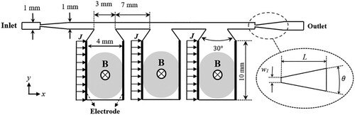
Table 1. The three-cavity MMR micropump variables.

Parameter	Value
B (T)	0.25
$I_0$ (A)	2
f (Hz)	10
s (mm)	8

The electric current applied to the first, second, and third cavities can be evaluated by the step functions given by Equations (1(1) $\begin{array}{rl}|I_1\left(t\right)|& =I_0\mathrm{s}\mathrm{g}\mathrm{n}\left(\cos \left(2\pi ft\right)\right)\end{array}$(1) ), (2(2) $\begin{array}{rl}|I_2\left(t\right)|& =I_0\mathrm{s}\mathrm{g}\mathrm{n}\left(\cos \left(2\pi ft-\mathrm{\Delta }\varphi \frac{\pi }{180}\right)\right)\end{array}$(2) ), and (3(3) $\begin{array}{rl}|I_3\left(t\right)|& =I_0\mathrm{s}\mathrm{g}\mathrm{n}\left(\cos \left(2\pi ft-2\mathrm{\Delta }\varphi \frac{\pi }{180}\right)\right)\end{array}$(3) ), respectively, as a function of the excitation frequency and phase difference. There is no difference between the applied electric current, except for their lag phase difference. The phase difference leads to a delay between the motions of the mercury slugs. (1) $\begin{array}{rl}|I_1\left(t\right)|& =I_0\mathrm{s}\mathrm{g}\mathrm{n}\left(\cos \left(2\pi ft\right)\right)\end{array}$(1) (2) $\begin{array}{rl}|I_2\left(t\right)|& =I_0\mathrm{s}\mathrm{g}\mathrm{n}\left(\cos \left(2\pi ft-\mathrm{\Delta }\varphi \frac{\pi }{180}\right)\right)\end{array}$(2) (3) $\begin{array}{rl}|I_3\left(t\right)|& =I_0\mathrm{s}\mathrm{g}\mathrm{n}\left(\cos \left(2\pi ft-2\mathrm{\Delta }\varphi \frac{\pi }{180}\right)\right)\end{array}$(3) Figure 2 illustrates an operation cycle of the micropump with a lagging phase difference of ${90}^{\circ }$, 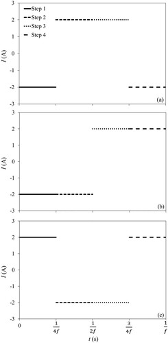where the arrangements of the mercury slugs at the beginning of the four steps of the cycle, are shown. Figure 3(a–c) also show the variations of the AC electric current applied to the first, second, and third mercury slugs during the four steps of the corresponding pumping cycle.

Figure 2. A schematic of the three-cavity MMR micropump at the beginning of the four steps of a pump cycle.

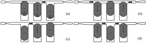
Figure 3. The electric current imposed to the (a) first, (b) second, and (c) third mercury slug during the four steps of the MMR micropump pumping cycle with $\mathrm{\Delta }\varphi ={90}^{\circ }$. When the current is in the $+x$ and $-x$ direction, it has a positive and negative sign, respectively.

At the beginning of step 1, the first mercury slug is at its highest position with zero velocity as shown in Figure 2(a), and is going to start a downward motion as a result of a downward Lorentz force generated in the slug due to an electric current imposed in the $-x$ direction during step 1 as shown in Figure 3(a). Figure 2(b) shows the position of the slugs at the beginning of step 2 when the first slug is at the middle of its cavity with its maximum downward velocity. As a result of an upward Lorentz force during step 2 (see Figure 3(a)), its velocity decreases to be stopped at its lowest position at the end of step 2 (beginning of step-3) shown in Figure 2(c). During step 3, an upward Lorentz force is applied to the first slug (see Figure 3(a)) so that it will be at the middle of its cavity with its maximum upward velocity at the beginning of step 4. As shown in Figure 3(a), during step 4, a downward Lorentz force is applied to the first slug decelerating the slug to be stopped at its highest position in the cavity. At the end of step 4, the slug is at the same position as it was at the first step when the pumping cycle is restarted. The reciprocating motion of the mercury slugs in their cavities lead to the pumping of air from the inlet to the outlet of the micropump.

2.1. Numerical procedure

2.1.1. Numerical model

To investigate the performance of the micropump, a two-dimensional geometry of the three-cavity MMR micropump, similar to the geometry shown in Figure 1, was generated. The two-dimensional simulations of the micropump were performed through interFoam solver of the OpenFOAM code where interfaces between air and mercury phases are captured by the volume of fluid (VOF) two-phase approach, where Equation (4(4) $\begin{array}{rl}\frac{\mathrm{\partial }\alpha }{\mathrm{\partial }t}+\mathrm{\nabla }.\left(\alpha \overrightarrow{v}\right)& =0\end{array}$(4) ) is solved to track interfaces. InterFoam solver solves the continuity (Equation (5(5) $\begin{array}{rl}\mathrm{\nabla }.\overrightarrow{v}& =0\end{array}$(5) )) and Navier-Stokes equations (Equation (6(6) $\begin{array}{rl}\frac{\mathrm{\partial }}{\mathrm{\partial }t}\left(\rho \overrightarrow{v}\right)+\mathrm{\nabla }\cdot (\rho \overrightarrow{v}\otimes \overrightarrow{v})& =-\overrightarrow{\mathrm{\nabla }}p+\mu {\mathrm{\nabla }}^2\overrightarrow{v}\\ & +\frac{1}{3}\mu \mathrm{\nabla }\left(\mathrm{\nabla }\cdot \overrightarrow{v}\right)+\rho \overrightarrow{g}+{\overrightarrow{f}}_{\sigma }+{\overrightarrow{F}}_{\mathrm{L}}\end{array}$(6) )) for two immiscible and incompressible fluids, where at each cell, the material properties are quantified by Equation (7(7) $\begin{array}{rl}\rho & =\alpha {\rho }_{mercury}+(1-\alpha ){\rho }_{air}\end{array}$(7) ) as a function of the primary fluid (mercury) volume fraction. (4) $\begin{array}{rl}\frac{\mathrm{\partial }\alpha }{\mathrm{\partial }t}+\mathrm{\nabla }.\left(\alpha \overrightarrow{v}\right)& =0\end{array}$(4) (5) $\begin{array}{rl}\mathrm{\nabla }.\overrightarrow{v}& =0\end{array}$(5) (6) $\begin{array}{rl}\frac{\mathrm{\partial }}{\mathrm{\partial }t}\left(\rho \overrightarrow{v}\right)+\mathrm{\nabla }\cdot (\rho \overrightarrow{v}\otimes \overrightarrow{v})& =-\overrightarrow{\mathrm{\nabla }}p+\mu {\mathrm{\nabla }}^2\overrightarrow{v}\\ & +\frac{1}{3}\mu \mathrm{\nabla }\left(\mathrm{\nabla }\cdot \overrightarrow{v}\right)+\rho \overrightarrow{g}+{\overrightarrow{f}}_{\sigma }+{\overrightarrow{F}}_{\mathrm{L}}\end{array}$(6) (7) $\begin{array}{rl}\rho & =\alpha {\rho }_{mercury}+(1-\alpha ){\rho }_{air}\end{array}$(7) In Equation (6(6) $\begin{array}{rl}\frac{\mathrm{\partial }}{\mathrm{\partial }t}\left(\rho \overrightarrow{v}\right)+\mathrm{\nabla }\cdot (\rho \overrightarrow{v}\otimes \overrightarrow{v})& =-\overrightarrow{\mathrm{\nabla }}p+\mu {\mathrm{\nabla }}^2\overrightarrow{v}\\ & +\frac{1}{3}\mu \mathrm{\nabla }\left(\mathrm{\nabla }\cdot \overrightarrow{v}\right)+\rho \overrightarrow{g}+{\overrightarrow{f}}_{\sigma }+{\overrightarrow{F}}_{\mathrm{L}}\end{array}$(6) ), ${\overrightarrow{f}}_{\sigma }$ and ${\overrightarrow{F}}_{\mathrm{L}}$ are the surface tension and Lorentz forces, respectively. The surface tension is evaluated by (8) ${\overrightarrow{f}}_{\sigma }=\sigma \kappa \mathrm{\nabla }\alpha ,$(8) where (9) $\kappa =-\mathrm{\nabla }.\hat{n},$(9) and (10) $\hat{n}=\frac{\mathrm{\nabla }\alpha }{|\mathrm{\nabla }\alpha |}.$(10) The Lorentz forces imposed on the mercury slugs are evaluated by (11) ${\overrightarrow{F}}_{\mathrm{L}}=\overrightarrow{J}\times \overrightarrow{B},$(11) where (12) $\overrightarrow{J}=\frac{\overrightarrow{I}}{A}.$(12) Since a constant current electrical supply and permanent magnets were used in the micropump, the magnitude of the electric current and the magnetic field was assumed to be constant as listed in Table 1.

To solve the equations, the PISO scheme was used as the pressure velocity coupling algorithm, the Euler implicit was employed as the temporal discretization, Gauss cell-based linear option was selected as the gradient scheme, Gauss upwind was used to discretizing the convection term of the Navier-Stokes equations, Gauss second-order Van Leer was used to discretizing the convection term of the volume fraction equation, and Gauss linear corrected option was chosen as the Laplacian scheme. The criteria of the pressure and the velocity residuals were set to ${10}^{-7}$ and ${10}^{-6}$, respectively. The physical properties of air and mercury used in the simulations were tabulated in Table 2.

Table 2. Physical properties of air and mercury at ${25}^{\circ }\mathrm{C}$.

Property	Mercury	Air
$\rho (\mathrm{k}\mathrm{g}/{\mathrm{m}}^3$)	13,567	0.1855
$\mu (\mathrm{P}\mathrm{a}.\mathrm{s})$	$1.52\times {10}^{-3}$	$1.85\times {10}^{-5}$
$\sigma \left(\mathrm{N}/\mathrm{m}\right)$	0.4855
$\theta {}_{\mathrm{s}}{(}^{\circ })$	135

In the simulations, for the momentum equations, a pressure inlet/outlet boundary condition was applied at the inlet/outlet of the micropump and the inlet of the mercury cavities. The no-slip wall velocity boundary condition was applied for the microchannel and cavity boundaries. A zero gauge pressure was assumed at the inlet of the micropump and the mercury cavities, but at the outlet of the micropump, different pressure values were imposed depending on the back-pressure.

2.1.2. Computational grid and time step sensitivity study

When an Eulerian interface capturing (e.g. VOF) is used in multiphase simulations, it is essential to ensure that the computational grid is refined enough to accurately capture interfaces. Increasing the grid resolution reduces the width of the interfaces and improves the accuracy of numerical results, but also significantly increases computational expenses. Therefore, a grid sensitivity analysis was performed on the micropump with no valve by generating four cases with computational grid cells of 17,880, 40,302, 72,100, and 161,790 to find the optimum grid resolution. The mean flow rate predictions of the first two cycles of the micropump at a zero back-pressure, while the phase difference and frequency were assumed to be ${90}^{\circ }$ and 10 Hz, resulted from the four grids are tabulated in Table 3, and the volume fraction contours of the third slug at 0.03 s concluded from the different grids are illustrated in Figure 4, when the third slug of the micropump entered into the air microchannel. Figure 4(a,b) indicate that the width of the interface is large in relative to the curvature of the interface, so it was concluded that the grids of cases 1 and 2 were not sufficiently refined. Table 3 clarifies the differences between the mean pumping flow rate of the micropump estimated for cases 3 and 4 were negligible. Consequently, it was concluded that the grid with 72,100 cells was an acceptable grid for simulations of the MMR micropump.

Figure 4. The volume fraction contours, where the red and blue colors represent volume fractions of 1 (mercury) and 0 (air), respectively, for the four cases with (a) 17,880, (b) 40,302, (c) 72,100, and (d) 161,790 number of cells.

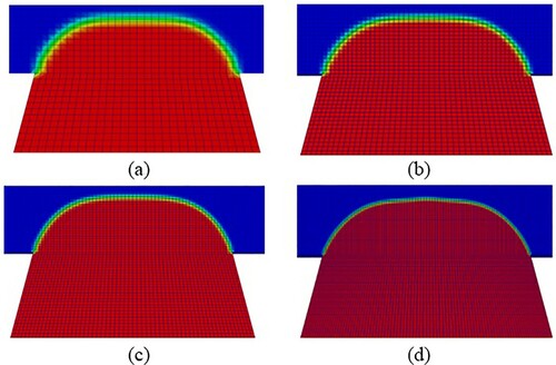
Table 3. Computational grid sensitivity study data.

Case	Number of cells	Mean pumping flow rate (mL/min)	The differences in flow rate (%)
1	17,880	9.15	−
2	40,302	8.50	7.6
3	72,100	8.15	4.3
4	161,790	8.04	1.4

The transient interFoam solver of the OpenFOAM code was used with an explicit MULES algorithm where the time step is set based on an upper limit of Courant number. With the explicit approach, the Courant number of the simulations needs to be limited to stabilize the simulations and get accurate predictions. To examine the influence of the maximum Courant number on the simulations, the three-cavity MMR micropump was simulated by three different maximum allowable Courant numbers listed in Table 4. In the table, the estimations of the mean pumping flow rate of the initial two cycles of the micropump as if different values were set for the upper limit of the Courant number, and the relative differences between the estimations are listed. Since the differences between the estimations of Cases 2 and 3 is negligible, 0.4 could be selected as the value of the maximum allowable Courant number. However, the maximum Courant number is usually picked less than 0.25 for the stability of simulations performed with the Explicit approach. Considering the stability and the results for the mean pimping flow rates tabulated in Table 4, a value of 0.2 was set as the upper limit of the Courant number for the current simulations.

Table 4. The micropump mean pumping flow rate predictions based on different maximum Courant numbers.

Case	Maximum allowable Courant number	The mean pumping flow rate (mL/min)	The differences in the flow rates (%)
1	1	7.68	–
2	0.4	8.13	5.54
3	0.2	8.15	0.25

3. Results and discussion

3.1. Numerical validation

The MMR micropump with the specifications listed in Table 5 was simulated by the interFoam solver of the OpenFOAM code, and the mean pumping flow rates at different back-pressures were evaluated and compared with the experimental measurements (Karmozdi et al., 2013) in Figure 5(a). This figure shows the numerical results and the experimental data are in reasonable agreement, while the numerical predictions overestimated the experimental results. The discrepancies can be due to the two-dimensional assumption of the numerical simulations, where the drag force and boundary layer effects on the top and bottom walls were ignored, leading to underestimation of the pressure drops, which could result in overestimation of the pumping flow rate of the micropump. In addition, liquids with high surface tensions (e.g. mercury) are not able to fill corners of capillaries with sharp angles, similar to what is shown in Figure 5(b). The possible gaps between mercury slugs and the cavity wall could result in leakage of the working flow from the front to the back of the mercury slugs. It is not feasible, however, to capture these gaps in two-dimensional geometries and model leakages in current numerical simulations, which is another factor that may also account for the overestimation of the flow rate by the numerical model.

Figure 5. (a) The comparison of the MMR micropump pumping flow rate estimated by the numerical estimations with the experimental measurements (Karmozdi et al., 2013) at different back-pressures. (b) A schematic of a mercury slug in a rectangular channel.

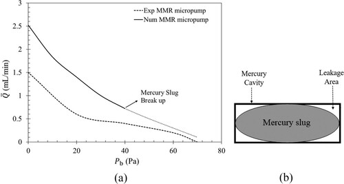
Table 5. The experimental prototype variables.

Parameter	Value
B (T)	0.2
$I_0$ (A)	1.5
f (Hz)	9
$\mathrm{\Delta }\varphi$ (${}^{\circ }$)	90
s (mm)	2

Despite the approximations in the numerical approach, there is reasonable agreement between the numerical predictions of the mean pumping flow rate of the MMR micropump and the experimental measurements, which confirms the accuracy of the numerical procedure. In addition, a good agreement was found between the interFoam solver and earlier numerical predictions of the Rayleigh–Taylor instability problem.

3.2. Influence of electric current phase difference

The electric current phase difference included in Equations (1(1) $\begin{array}{rl}|I_1\left(t\right)|& =I_0\mathrm{s}\mathrm{g}\mathrm{n}\left(\cos \left(2\pi ft\right)\right)\end{array}$(1) ) and (2(2) $\begin{array}{rl}|I_2\left(t\right)|& =I_0\mathrm{s}\mathrm{g}\mathrm{n}\left(\cos \left(2\pi ft-\mathrm{\Delta }\varphi \frac{\pi }{180}\right)\right)\end{array}$(2) ) leads to a delay in the movement of the slugs. Consequently, the first slug leads the second and third slugs, and the second slug leads the third slug. The value of the phase difference between the motion of the slugs dramatically affects the performance of the micropump, and it is necessary to find the best phase difference value of the micropump. To highlight the influence of the phase difference on the performance of the micropump, the flow rate at the outlet of the micropump at a back-pressure of 10 Pa was evaluated assuming the phase difference was 90${}^{\circ }$ and 120${}^{\circ }$ and plotted in Figure 6. As seen in the figure, during some time intervals (e.g. 0.05–0.09 s), the flow rate of the micropump goes to large negative values (e.g. −80 mL/min) as a result of a reverse flow from the outlet with a higher pressure (10 Pa) to the inlet of the micropump at atmospheric conditions (0 Pa). Exploring the results clarified that the reverse flows occur at time intervals during which the air microchannel is free of slugs so that air can penetrate from the outlet to the inlet leading to a reduction of the net pumping flow rate and efficiency of the micropump. However, since during a pumping cycle with a phase difference of 120${}^{\circ }$, the air microchannel is constantly closed by at least one of the slugs, there is no reverse flow from the outlet to the inlet as shown in the figure. It should be noted that the negative outlet flow rates at some time intervals of the case with a phase difference of 120${}^{\circ }$ are due to the suction pressure imposed to the outlet section by the third slug during its downward motion, and it does not lead to a reverse flow from the outlet to the inlet.

Figure 6. The comparison of the outlet flow rate of the MMR micropump with an excitation frequency of 10 Hz at a back-pressure of 10 Pa when the phase difference value is 90${}^{\circ }$ and 120${}^{\circ }$.

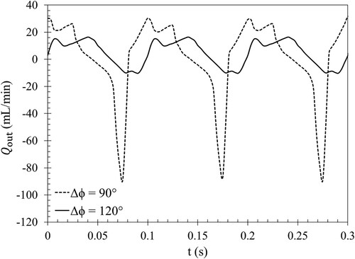
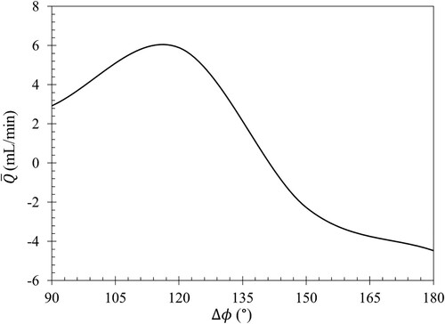
Figure 7 shows the variations of the mean pumping flow rate of the micropump at a back-pressure of 10 Pa as a function of the phase difference. According to the figure, the flow rate is positive when the phase difference is between 90${}^{\circ }$ to 140${}^{\circ }$ and is negative for larger phase differences. The figure clarifies the micropump has the best performance with the maximum mean flow rate of 5.9 mL/min when the phase difference is 120${}^{\circ }$.

Figure 7. The variation of the mean flow rate of the MMR micropump with an excitation frequency of 10 Hz at a back-pressure of 10 Pa as a function of the electric current phase difference.

Another reason for slugs' deformation is their dynamic interaction. For a phase difference of 90${}^{\circ }$, the slugs are not in the microchannel at the same time, so the asymmetric shape of the slugs is not as high as that of 120${}^{\circ }$, and the interruption does not happen for a back-pressure of 20 Pa.

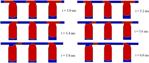
It was found that the micropump does not properly operate with phase differences smaller than 80${}^{\circ }$ when there is a smaller delay between the mercury slugs' motion, and the tip of two or even three slugs can simultaneously penetrate the air microchannel. Accordingly, when a slug moves downward, it can pull the tip of the other penetrated slugs towards itself, or when it moves upward, it can push the tip of the penetrated slugs away from itself. Either pulling or pushing of the penetrated tips intensifies the asymmetric shape of the penetrated portion of the slugs in the air microchannel and increases the possibility of detaching the penetrated parts from the rest of the slugs. As an example, Figure 8 shows the operation of the micropump with a frequency and phase difference of 10 Hz and 30${}^{\circ }$, where all the three slugs have penetrated the air microchannel at 5 ms and a downward motion of the second slug pulls the tip of the first slug towards itself and splits it from the rest of the slug.

Figure 8. The mercury slugs configuration during the operation of the micropump with a frequency of 10 Hz and a phase difference of 30${}^{\circ }$ at a back-pressure of 10 Pa.

3.3. Influence of back-pressure

The back-pressure could influence the performance of the micropump in two ways. It could change the shape of the slugs in the microchannel which could adversely affect the micropump operation. Figure 9 presents the pressure contours of the micropump when the first mercury slug has entered into the air microchannel, while a back-pressure of 30 Pa is applied to the outlet. The figure shows that the first slug meets the inlet pressure on its left side and the outlet pressure on its right side. The larger value of the outlet pressure makes the slug penetrate more towards the inlet side (the left side) leading to an asymmetrical shape of the slug in the microchannel. The asymmetry shape of the slugs is more pronounced for higher back-pressures which can lead to breaking up of the mercury slugs and interruption of the micropump operation, similar to what happened at 40 Pa (see Figure 5) for the micropump studied in Section 3.1.

Figure 9. A snapshot at 0.14 s of the pressure contours of the micropump with a frequency of 10 Hz and a phase difference of 120${}^{\circ }$ at a back-pressure of 30 Pa.

The back-pressure could also lead to reverse flows from the outlet to the inlet of the micropump resulting in lower or even negative mean pumping flow rates. To clarify the influence of the back-pressure on the micropump performance, the time evolution of the outlet flow rate of the micropump with a frequency of 10 Hz was evaluated as a function of the back-pressure for phase differences of 90${}^{\circ }$ and 120${}^{\circ }$, and plotted in Figure 10(a,b), respectively. As discussed earlier in Section 3.2, during a pumping cycle of the micropump with a phase difference of 90${}^{\circ }$, there are time intervals during which the air microchannel is free of mercury. Consequently, as seen in Figure 10(a), there is a reverse flow at back-pressures of 5, 10, and 20 Pa. Therefore, for the micropump with a phase difference of 90${}^{\circ }$, the mean flow rate is reduced for higher back-pressures. However, as seen in Figure 10(b), there is no reverse flow in the pumping cycle of the micropump with a phase difference of 120${}^{\circ }$ at back-pressures of 0, 5, and 10 Pa as the microchannel is clogged by a mercury slug during the pumping cycle (see Section 3.2). At back-pressures more than 20 Pa, the asymmetric deformations of the slugs, as previously discussed, result in a break-up of the mercury slugs in the air microchannel interrupting the operation of the micropump.

Figure 10. The time evolution of the outlet flow rate of the three-cavity MMR micropump with a phase difference of (a) 90${}^{\circ }$ and (b) 120${}^{\circ }$ and an excitation frequency of 10 Hz as a function of back-pressure.

Figure 11 shows the mean flow rate of the three-cavity MMR micropump at different back-pressures for phase differences of 90${}^{\circ }$ and 120${}^{\circ }$. As shown in the figure, except at very low back-pressures, the flow rate is larger for a phase difference of 120${}^{\circ }$. The figure reveals that the flow rate of the micropump with a phase difference of 90${}^{\circ }$ constantly decreases by back-pressure from 8.4 mL/min at a back-pressure of 0 Pa to 0 mL/min at a back-pressure of 17.8 Pa. Nonetheless, the mean flow rate of the micropump with a 120${}^{\circ }$ phase difference is not significantly changed by back-pressures less than 10 Pa, in that the air microchannel is closed by at least one of the slugs during a pumping cycle. However, based on the results, which were not reported here for the sake of brevity, the increase of the back-pressure reduces the penetration of the slugs into the microchannel; hence for back-pressures larger than 10 Pa, there are time intervals during which the microchannel is free of slugs which leads to reverse flows from the outlet to the inlet and reducing the net pumping flow rate. At back-pressures larger than 20 Pa, the mercury slug breaks up, causing interruptions in the micropump operation.

Figure 11. The mean flow rate of the micropump with an excitation frequency of 10 Hz as a function of the back-pressure for phase differences of 90${}^{\circ }$ and 120${}^{\circ }$.

3.4. Three-cavity MMR micropump with a diffuser/nozzle valve

As discussed earlier, during a pumping cycle of the micropump with a phase difference of 90${}^{\circ }$, there are periods when none of the slugs closes the air microchannel causing reverse flows from the outlet to the inlet, and reducing the pumping flow rate of the micropump at large back-pressures. Accordingly, in this section, the possibility of implementing a diffuser/nozzle valve at the inlet and outlet of the micropump to mitigate the adverse effect of the reverse flow on the micropump performance was investigated.

A diffuser/nozzle valve acts as a diffuser or nozzle depending on the flow direction passing through it. The pressure drop along a diffuser/nozzle valve is smaller when the flow is in the direction that the valve acts as a diffuser (Jiang et al., 1998; Olsson et al., 2000; W. Wang et al., 2008). Therefore, in the three cavity MMR micropump with a diffuser/nozzle valve (see Figure 1), when there is a reverse flow from the outlet to the inlet, both the inlet and outlet valves behave as a nozzle so that the pressure drop is larger between the outlet and inlet compared to the MMR micropump with no valve. In addition, when the air microchannel is free of mercury slugs and the movements of mercury slugs result in incoming airflow from the inlet and outlet, more air is sucked in from the inlet acting as a diffuser with a smaller pressure drop. However, when the movements of mercury slugs result in outgoing airflow from the inlet and outlet, more air passes through the outlet acting as a diffuser with a smaller pressure drop. The larger incoming airflow from the inlet and the larger outgoing airflow from the outlet, results in pumping air from the inlet to the outlet.

The difference between the pressure drop of the valve as it acts a diffuser or nozzle is a function of its geometry (Jiang et al., 1998). To find the best geometrical configurations for the diffuser/nozzle valve used in the MMR micropump, the reverse flow from the outlet to the inlet along the air microchannel at a back-pressure of 1.2 Pa was quantified, while the diffuser/nozzle valves, listed in Table 6, were implemented at the inlet and outlet of the air microchannel. To explore the geometry of the valve, the width of the larger section was assumed to be equal to 1 mm to limit the dimension of the air microchannel, and the neck width ($w_1$) was assumed to be more than 120 $\mu \mathrm{m}$ to consider its fabrication feasibility (Karmozdi et al., 2013). The comparison of the reverse flow listed in Table 6 indicates that the diffuser/nozzle valve with a length of 5 mm and an angle of 10${}^{\circ }$ has the best performance with the least reverse flow.

Table 6. The mean reverse flow rate of diffuser/nozzle valves at a back-pressure of 1.2 Pa as a function of their length and angle.

Case	L (mm)	θ (${}^{\circ }$)	Mean reverse flow rate (mL/min)
1	1	10	31.76
2	1	46	3.19
3	2.5	10	15.34
4	2.5	20	0.97
5	4	10	4.58
6	4	12	1.54
7	5	7	6.11
8	5	10	0.83
9	6	8.2	0.87

To examine the influence of implementing the valve on the performance of the micropump with a phase difference of 90${}^{\circ }$, the diffuser/nozzle valve with a length of 5 mm and an angle of 10${}^{\circ }$ were implemented at the inlet/outlet of the micropump, with the arrangement shown in Figure 2. The outlet flow rates of the three-cavity micropump with and without the diffuser/nozzle valve at back-pressures of 10 and 20 Pa with a phase difference of 90${}^{\circ }$ are compared in Figure 12. As seen in the figure, implementing the diffuser/nozzle valve prevented the reverse flow, which increased the mean flow rate of the micropump from 2.7 to 6.5 mL/min at a back-pressure of 10 Pa, and from −0.8 to 3.9 mL/min at a back-pressure of 20 Pa. Results also indicated that implementing the valve increased the maximum back-pressure, that the micropump can maintain, from 17.8 to 40 Pa.

Figure 12. Comparison of three-cavity MMR micropump with and without the diffuser/nozzle valve in frequency of 10 Hz and phase difference of 90${}^{\circ }$.

4. Conclusions

At a phase difference of 120${}^{\circ }$, the MMR micropump maintains a mean flow rate of 6.1 mL/min and a sustainable back-pressure of 20 Pa. However, changing the phase difference to 90${}^{\circ }$, reduced the mean pumping flow rate and sustainable back-pressure to 2.7 mL/min and 17.8 Pa, respectively as a result of the reverse flow from the outlet to the inlet. Implementing a diffuser/nozzle valve with a length of 5 mm and an angle of 10${}^{\circ }$ into the micropump working at phase difference of 90${}^{\circ }$, prevented the reverse flow, and increased its mean flow rate and sustainable back-pressure to 6.5 mL/min and 40 Pa, respectively.

The performance of the MMR micropump could improve if the geometry of the air microchannel is modified so that the regular motion of mercury slugs is not interrupted at high back-pressures. In addition, the possibility of reducing the number of mercury cavities in order to reduce the size of the micropump can be explored. The investigations on air microchannel and mercury cavities are left for future work.

Acknowledgments

The authors would like to thank Prof. Goodarz Ahmadi for review of the manuscript and helpful comments.

Disclosure statement

No potential conflict of interest was reported by the author(s).

References

- Chandika S., Asokan R., & Vijayakumar K. (2012). Flow characteristics of the diffuser/nozzle micropump – A state space approach. Flow Measurement and Instrumentation, 28, 28–34. https://doi.org/https://doi.org/10.1016/j.flowmeasinst.2012.06.003
- Cui Q., Liu C., & Zha X. F. (2007). Study on a piezoelectric micropump for the controlled drug delivery system. Microfluidics and Nanofluidics, 3(4), 377–390. https://doi.org/https://doi.org/10.1007/s10404-006-0137-0
- Cui Q., Liu C., & X. F. Zha (2008). Simulation and optimization of a piezoelectric micropump for medical applications. The International Journal of Advanced Manufacturing Technology, 36(5), 516–524. https://doi.org/https://doi.org/10.1007/s00170-006-0867-x
- Dau V., & Dinh T. (2015). Numerical study and experimental validation of a valveless piezoelectric air blower for fluidic applications. Sensors and Actuators B: Chemical, 221, 1077–1083. https://doi.org/https://doi.org/10.1016/j.snb.2015.07.041
- Denishev K. H., & Trencheva B. B. (2007). Micropumps for medical applications. Electronics.
- Ez Abadi A. M., Sadi M., Farzaneh-Gord M., Ahmadi M. H., Kumar R., & Chau K. w. (2020). A numerical and experimental study on the energy efficiency of a regenerative heat and mass exchanger utilizing the counter-flow maisotsenko cycle. Engineering Applications of Computational Fluid Mechanics, 14(1), 1–12. https://doi.org/https://doi.org/10.1080/19942060.2019.1617193
- Fylladitakis E. D., Theodoridis M. P., & Moronis A. X. (2014). Review on the history, research, and applications of electrohydrodynamics. IEEE Transactions on Plasma Science, 42(2), 358–375. https://doi.org/https://doi.org/10.1109/TPS.27
- Heng K. H., Huang L., Wang W., & Murphy M. C. (1999). Development of a diffuser/nozzle-type micropump based on magnetohydrodynamic (MHD) principle. In Microfluidic devices and systems II (Vol. 3877, pp. 66–73).
- Huang L., Wang W., Murphy M., Lian K., & Ling Z. G.. (2000). LIGA fabrication and test of a DC type magnetohydrodynamic (MHD) micropump. Microsystem Technologies, 6(6), 235–240. https://doi.org/https://doi.org/10.1007/s005420000068
- Iverson B. D., & Garimella S. V. (2008). Recent advances in microscale pumping technologies: a review and evaluation. Microfluidics and Nanofluidics, 5(2), 145–174. https://doi.org/https://doi.org/10.1007/s10404-008-0266-8
- Jang J., & Lee S. S. (2000). Theoretical and experimental study of MHD (magnetohydrodynamic) micropump. Sensors and Actuators A: Physical, 80(1), 84–89. https://doi.org/https://doi.org/10.1016/S0924-4247(99)00302-7
- Jiang X., Zhou Z., Huang X., Li Y., Yang Y., & Liu C. (1998). Micronozzle/diffuser flow and its application in micro valveless pumps. Sensors and Actuators A: Physical, 70(1–2), 81–87. https://doi.org/https://doi.org/10.1016/S0924-4247(98)00115-0
- Karmozdi M., Afshin H., & Shafii M. B. (2020). Electrical analogies applied on MMR micropump. Sensors and Actuators A: Physical, 301, Article ID 111675. https://doi.org/https://doi.org/10.1016/j.sna.2019.111675
- Karmozdi M., Salari A., & Shafii M. B. (2013). Experimental study of a novel magneto mercury reciprocating (MMR) micropump, fabrication and operation. Sensors and Actuators A: Physical, 194, 277–284. https://doi.org/https://doi.org/10.1016/j.sna.2013.02.012
- Koombua K., & Pidaparti R. M. (2010). Performance evaluation of a micropump with multiple pneumatic actuators via coupled simulations. Engineering Applications of Computational Fluid Mechanics, 4(3), 357–364. https://doi.org/https://doi.org/10.1080/19942060.2010.11015323
- Laser D. J., & Santiago J. G. (2004). A review of micropumps. Journal of Micromechanics and Microengineering, 14(6), R35. https://doi.org/https://doi.org/10.1088/0960-1317/14/6/R01
- Lemoff A. V., & Lee A. P. (2000). An AC magnetohydrodynamic micropump. Sensors and Actuators B: Chemical, 63(3), 178–185. https://doi.org/https://doi.org/10.1016/S0925-4005(00)00355-5
- Lim S., & Choi B. (2009). A study on the MHD (magnetohydrodynamic) micropump with side-walled electrodes. Journal of Mechanical Science and Technology, 23(3), 739–749. https://doi.org/https://doi.org/10.1007/s12206-008-1107-0
- Liu Y., Komatsuzaki H., Imai S., & Nishioka Y. (2011). Planar diffuser/nozzle micropumps with extremely thin polyimide diaphragms. Sensors and Actuators A: Physical, 169(2), 259–265. https://doi.org/https://doi.org/10.1016/j.sna.2011.02.009
- Moghadam M. E., & Shafii M. B. (2010). Rotary magnetohydrodynamic micropump based on slug trapping valve. Journal of Microelectromechanical Systems, 20(1), 260–269. https://doi.org/https://doi.org/10.1109/JMEMS.2010.2090500
- Munih J., Hočevar M., Petrič K., & Dular M. (2020). Development of CFD-based procedure for 3d gear pump analysis. Engineering Applications of Computational Fluid Mechanics, 14(1), 1023–1034. https://doi.org/https://doi.org/10.1080/19942060.2020.1789506
- Nguyen N. T., Huang X., & Chuan T. K. (2002). MEMS-micropumps: a review. Journal of Fluids Engineering, 124(2), 384–392. https://doi.org/https://doi.org/10.1115/1.1459075
- Nisar A., Afzulpurkar N., Mahaisavariya B., & Tuantranont A. (2008). MEMS-based micropumps in drug delivery and biomedical applications. Sensors and Actuators B: Chemical, 130(2), 917–942. https://doi.org/https://doi.org/10.1016/j.snb.2007.10.064
- Olsson A., Stemme G., & Stemme E. (2000). Numerical and experimental studies of flat-walled diffuser elements for valve-less micropumps. Sensors and Actuators A: Physical, 84(1–2), 165–175. https://doi.org/https://doi.org/10.1016/S0924-4247(99)00320-9
- Pan Q. S., He L. G., Huang F. S., Wang X. Y., & Feng Z. H. (2015). Piezoelectric micropump using dual-frequency drive. Sensors and Actuators A: Physical, 229, 86–93. https://doi.org/https://doi.org/10.1016/j.sna.2015.03.029
- Pinilla J. A., Guerrero E., Pineda H., Posada R., Pereyra E., & Ratkovich N. (2019). CFD modeling and validation for two-phase medium viscosity oil-air flow in horizontal pipes. Chemical Engineering Communications, 206(5), 654–671. https://doi.org/https://doi.org/10.1080/00986445.2018.1516646
- Ramezanizadeh M., Alhuyi Nazari M., Ahmadi M. H., & Chau K. w. (2019). Experimental and numerical analysis of a nanofluidic thermosyphon heat exchanger. Engineering Applications of Computational Fluid Mechanics, 13(1), 40–47. https://doi.org/https://doi.org/10.1080/19942060.2018.1518272
- Richter A., & Sandmaier H. (1990). An electrohydrodynamic micropump. In IEEE proceedings on micro electro mechanical systems, an investigation of micro structures, sensors, actuators, machines and robots (pp. 99–104).
- Ritchie W. (1833). XV. Experimental researches in electro-magnetism and magneto-electricity. Philosophical Transactions of the Royal Society of London, 123, 313–321. https://doi.org/https://doi.org/10.1098/rstl.1833.0017
- Singh S., Kumar N., George D., & Sen A. (2015). Analytical modeling, simulations and experimental studies of a PZT actuated planar valveless PDMS micropump. Sensors and Actuators A: Physical, 225, 81–94. https://doi.org/https://doi.org/10.1016/j.sna.2015.02.012
- Singhal V., Garimella S. V., & Murthy J. Y. (2004). Low Reynolds number flow through nozzle-diffuser elements in valveless micropumps. Sensors and Actuators A: Physical, 113(2), 226–235. https://doi.org/https://doi.org/10.1016/j.sna.2004.03.002
- Smits J. G. (1990). Piezoelectric micropump with three valves working peristaltically. Sensors and Actuators A: Physical, 21(1–3), 203–206. https://doi.org/https://doi.org/10.1016/0924-4247(90)85039-7
- Stemme E., & Stemme G. (1993). A valveless diffuser/nozzle-based fluid pump. Sensors and Actuators A: Physical, 39(2), 159–167. https://doi.org/https://doi.org/10.1016/0924-4247(93)80213-Z
- Wang P. J., Chang C. Y., & Chang M. L. (2004). Simulation of two-dimensional fully developed laminar flow for a magneto-hydrodynamic (MHD) pump. Biosensors and Bioelectronics, 20(1), 115–121. https://doi.org/https://doi.org/10.1016/j.bios.2003.10.018
- Wang W., Zhang Y., Tian L., Chen X., & Liu X. (2008). Piezoelectric diffuser/nozzle micropump with double pump chambers. Frontiers of Mechanical Engineering in China, 3(4), 449–453. https://doi.org/https://doi.org/10.1007/s11465-008-0076-4
- Yang S., He X., Yuan S., Zhu J., & Deng Z. (2015). A valveless piezoelectric micropump with a Coanda jet element. Sensors and Actuators A: Physical, 230, 74–82. https://doi.org/https://doi.org/10.1016/j.sna.2015.04.016
- Yao Q., Xu D., Pan L., Melissa Teo A., Ho W., Peter Lee V., & Shabbir M. (2007). CFD simulations of flows in valveless micropumps. Engineering Applications of Computational Fluid Mechanics, 1(3), 181–188. https://doi.org/https://doi.org/10.1080/19942060.2007.11015191
- Zeng S., Chen C. H., Mikkelsen Jr J. C., & Santiago J. G. (2001). Fabrication and characterization of electroosmotic micropumps. Sensors and Actuators B: Chemical, 79(2–3), 107–114. https://doi.org/https://doi.org/10.1016/S0925-4005(01)00855-3
- Zhang X. Y., Jiang C. X., Lv S., Wang X., Yu T., Jian J., Shuai Z.-J., & Li W.-Y. (2021). Clocking effect of outlet RGVs on hydrodynamic characteristics in a centrifugal pump with an inlet inducer by CFD method. Engineering Applications of Computational Fluid Mechanics, 15(1), 222–235. https://doi.org/https://doi.org/10.1080/19942060.2021.1871961