Development and validation of a Riemann solver in OpenFOAM® for non-ideal compressible fluid dynamics

ABSTRACT

Recently, there is an increased interest in supercritical CO₂ and organic Rankine cycles (ORC) for their ability to achieve higher thermodynamic efficiency. However, the non-ideal gas thermodynamic in these cycles may affect the flow properties critically, necessitating the research of non-ideal compressible fluid dynamics (NICFD). Thus, simulation tools that can accurately predict fluid flows with NICFD are significant. This study presents a new approximation Riemann solver in OpenFOAM for NICFD. The new solver uses a real-gas (look-up table based) approximate Riemann flux calculator (modified from HLLC ALE flux calculator) through adding a new thermodynamic library tightly coupled with the OpenFOAM®. To validate the solver, three cases are presented, including a NASA transonic nozzle operating with air, to confirm the ability to correctly simulate the transonic flow phenomena and the shock waves; the VKI 2D cascade operated with MDM to assess the ability in simulating non-ideal gas flows typically to industrial applications; and the dense gas flow (MD₄M) passing a backward ramp to illustrate the ability of the flux calculator and look-up table mechanism that can work well in the non-ideal region of fluid properties. This study can benefit future engineering applications of computational fluid mechanics of NICFD and the OpenFOAM community.

KEYWORDS:

• OpenFOAM
• compressible flow
• Riemann solver
• look-up table equation of state
• non-ideal compressible fluid dynamics

1. Introduction

Owing to their ability to achieve higher thermodynamic efficiency, there has been increased interest in transcritical and supercritical cycles for the conversion of thermal energy (heat) to shaft power. The Supercritical Carbon Dioxide (${\mathrm{s}\mathrm{C}\mathrm{O}}_2$) power cycle and Rankine cycles using organic fluids (ORCs) are two types of these cycles.

The ${\mathrm{s}\mathrm{C}\mathrm{O}}_2$ power cycle has attracted substantial attention in recent years, owing to its compactness, higher efficiency and simpler cycle layout (Dostal et al., 2004; Wang et al., 2015; Xu et al., 2019). ${\mathrm{s}\mathrm{C}\mathrm{O}}_2$ is regarded as an excellent working fluid owing to several advantages, such as an easily attainable critical point (7.38 MPa, 304.25 K) compared with ${\mathrm{H}}_2\mathrm{O}$ (22.064 MPa, 647.1 K) or other fluids, good availability, and low global warming potential compared with other gases. Today, several companies are working on large-scale axial ${\mathrm{s}\mathrm{C}\mathrm{O}}_2$ turbines demonstrations (Kalra et al., 2014; Wright et al., 2010). For power cycles in the range 0.1–25 MW using ${\mathrm{s}\mathrm{C}\mathrm{O}}_2$ allows a paradigm shift to using efficient radial inflow turbines (Qi et al., 2017). This is possible owing to the combined effects of the highly dense working fluid, comparably low flow rates, and low specific speeds, resulting in highly power-dense machines. A similar focus has been given to ORCs, which exploit their thermodynamic properties to ensure better matching between low-temperature heat sources and densely working fluids.

In these cycles, it is essential to pay attention to non-ideal gas thermodynamic phenomena. Especially for ${\mathrm{s}\mathrm{C}\mathrm{O}}_2$ compressors, whose operating conditions are near the critical point, non-ideal gas dynamics for ${\mathrm{s}\mathrm{C}\mathrm{O}}_2$ significantly affect the flow properties. Similarly, in high-pressure-ratio ORC turbines, it is common that shock waves appear when flow passes through turbomachinery channels. They are the consequences of sudden expansions in nozzles or at blade tips. Unless these components can be simulated and designed appropriately, all gains in cycle efficiency will be lost due to poor component performance. Hence, the necessity to predict fluid flow accurately under these non-ideal conditions, to capture the actual characteristics of dense/supercritical fluids correctly, to solve compressible high Mach number flows whose thermodynamic behaviors differ from perfect gas relations, have led research into the area of Non-Ideal Compressible Fluid Dynamics (NICFD).

In the design stage, accurate NICFD simulations are essential for the s${\mathrm{C}\mathrm{O}}_2$ cycle and ORC components that operate in the supercritical region or close to the critical points. Numerical solutions for these highly compressible flows, using Computational Fluid Dynamics (CFD), have been reported by several authors (Gori, 2019; Qiu, 2021; Vitale et al., 2017); however, most of these studies have used numerical methods developed for perfect gases (Drikakis & Tsangaris, 1993). Hence, ORC turbomachinery requires appropriate simulation tools (Colonna et al., 2006; Head et al., 2016). For both the ORC and ${\mathrm{s}\mathrm{C}\mathrm{O}}_2$ research fields, reliable NICFD simulations of such flows still represent a challenge, as sophisticated tools coupled with highly complex and experimentally calibrated thermodynamic models are needed. Thus, there is a necessity for simulation tools that can accurately predict flows of non-ideal fluids during the design stage.

In practical applications, it is quite common to carry out CFD simulations of such flows using the perfect gas relations with modified gas constants and isentropic coefficients. However, these assumptions can introduce errors, owing to the limited accuracy of the approximation of gas properties. In some cases, changes in basic design parameters are observed (Jassim et al., 2008) owing to different gas models. This is especially important when studying compressible flows with properties in the non-ideal gas region, where non-ideal gas phenomena can alter the flow relationships. Poor evaluation of total pressure and temperature values leads to a poor prediction of losses, specific work, heat exchange and density, which influence the computation of momentum components and, consequently, the predicted flow structure (Jassim et al., 2008). Thus it is essential for CFD solvers to use the most accurate real gas properties to solve flows correctly (Ghalandari et al., 2019; Salih et al., 2019).

Several CFD solvers exist to solve NICFD problems, including ANSYS, SU2 and zFlow (Colonna & Rebay, 2004; Head et al., 2017; Vitale et al., 2015). SU2 obtains real gas properties by selecting a polytropic Equation of State (EoS), e.g. the polytropic ideal gas, polytropic Van der Waals or polytropic Peng–Robinson models. When solving the Riemann problem, the Vinokur–Montagnè approximate Riemann solver with the averaged-gradient formulation for the viscous counterpart is used (Vitale et al., 2015). In the most recent work, SU2 (v6.1.0) has been validated by comparing the numerical data with experimental results from the Test-Rig for Organic VApours (TROVA) (Gori et al., 2017). zFlow simulates inviscid dense gas flows with real gas properties calculated from the Peng–Robinson real gas equation of state. Flux is calculated by a Roe approximate Riemann flux calculator.

The current project uses OpenFOAM${}^{\circledR }$, a leading open-source project for continuum mechanics and CFD applications to address NICFD problems. Using OpenFOAM gives high reuse and development potential. OpenFOAM consists of a flexible framework to combine the required tools and libraries to solve CFD problems (He et al., 2013). The ability to link mathematical/numerical tools with physical models using the OpenFOAM C++ language allows the rapid development of different solvers and utilities.

Currently, OpenFOAM has several methods for capturing non-ideal gas properties. The existing thermophysical libraries include the following non-ideal equations of state: Peng–Robinson (PR), Redlich–Kwong (RK) and polynomial transport and thermodynamic properties (Weller et al., 1998). However, for the turbomachinery simulations in ${\mathrm{s}\mathrm{C}\mathrm{O}}_2$ or ORC applications, a fast non-ideal gas flow solver, coupled with a non-ideal gas Riemann flux calculator with the ability to select any gas model, is required. Currently, none of the existing solvers in OpenFOAM provide the ability to solve compressible Riemann problems and to use non-ideal equations of state at the same time. Furthermore, the implemented non-ideal equation of state requires iterative solutions, leading to a large computational burden and a slow solution process (Pini et al., 2015).

This work develops a fast solver and Riemann flux calculator that can accurately capture non-ideal fluid properties and transport properties, be not restricted to a specific gas model, and can correctly resolve shock and expansion waves in NICFD problems.

To achieve high speed and flexibility for gas models, a gas property look-up table that can be populated from any gas model is implemented (as shown in Appendix 2), which is similar to the built-in capabilities of some other solvers, e.g. ANSYS, CFX or Eilmer4. Similarly, the flux calculator has to be agnostic w.r.t. the gas model. Popular flux calculators (e.g. Roe, AUSM) are difficult to use, since they rely on ideal or polytropic EoSs to re-construct interface properties. Instead, the HLLC ALE flux calculator, whose interface properties can be calculated through a simple averaged method rather than through an ideal or polytropic EoS, is implemented (Luo et al., 2004).

This article is organized as follows. Section 2 describes the governing equations for the newly developed solver and the non-ideal gas HLLC ALE flux calculator. Section 3 presents three test cases to verify and validate the solver, and to demonstrate its capability. Finally, Section 4 finishes with concluding remarks.

2. Numerical methods and tools

In this section, the simulation tool OpenFOAM is introduced and the formulations of thermodynamic properties and the governing equations are discussed. This is followed by the theory of the non-ideal HLLC ALE scheme, which allows the solver to calculate non-ideal Riemann fluxes at the interface, without requiring a polytropic equation of state to reconstruct interface properties. Finally, the governing equations and workflow of the new solver Real Gas Density based Foam (RGDFoam) are introduced.

2.1. Simulation tools

The development of the simulation tool is done using the OpenFOAM extend project, version 3.0(Jasak, 2013). The OpenFOAM extend project is a fork of the OpenFOAM source code library. The OpenFoam extend project provides additional features including dynamic mesh, General Grid Interpolation (GGI) and mixing planes (Beaudoin & Jasak, 2008; Jasak & Beaudoin, 2011) that provide additional capabilities for future simulations targeted at non-ideal fluid turbomachinery.

2.2. Thermophysical and transport models for real gas properties

For the original ideal gas thermophysical model, the state of the fluid is univocally determined by the ideal gas equations of state, such as (1) $\begin{array}{rl}p& =\rho RT\end{array}$(1) (2) $\begin{array}{rl}h& =C_{p}T\end{array}$(2) Alternatively, the fluid state can be calculated by more general and complex non-ideal equations of state like those of PR, RK, Soave–Redlich–Kwong and Aungier–Redlich–Kwong (The OpenFOAM Foundation, 2016). However, the complex non-ideal equations of state need to be solved iteratively for every cell and every iterative step in order to calculate the current fluid states. Especially close to the critical point, where multiple iterations are required, this can lead to a significant increase in computational cost.

An alternative to solving the EoS that is done regularly (Loewenberg et al., 2008; Pini et al., 2015; Smith et al., 2006; Zhan & Sapatnekar, 2005) is to use a look-up table (LuT). Calling the LuT functions $\mathbf{L}$, which interpolates on a-priori calculated tables of fluid properties, avoids the need to iterate. As long as the interpolation process is fast, this leads to a substantial calculation speed-up. In this approach, the original thermophysical models and transport property models are replaced with respective functions (3) $\begin{array}{r}{\mathrm{\Phi }}_3={\mathbf{L}}_{{\mathrm{\Phi }}_3}({\varphi }_1,{\varphi }_2)\end{array}$(3) where $\mathbf{L}$ denotes the substitution function. This look-up table approach makes use of the fact that, once two-state properties (e.g. ${\varphi }_1$ and ${\varphi }_2$) are known, all other state properties (e.g. ${\mathrm{\Phi }}_3$) can be calculated. Depending on the solver formulation, look-up table functions may be required for specific enthalpy h, specific heat capacities $C_p$ and $C_v$, density ρ, ratio of specific heats γ, kinematic viscosity ν, and acoustic speed a.

The look-up tables are generated through a tabular data generator, the details of which are described in Appendix 2. When creating LuTs, three issues need to be considered: the maximum error introduced by the interpolation; table size (the resolution of tabular data nodal points); and self-consistency. In particular, self-consistency is such that, if using two different function calls, the outcome should be consistent, i.e. (4) $\begin{array}{rl}{\varphi }_1^{\prime }& =\mathbf{L}({\varphi }_2,{\varphi }_3)\end{array}$(4) (5) $\begin{array}{rl}{\varphi }_2^{\prime }& =\mathbf{L}({\varphi }_3,{\varphi }_1)\end{array}$(5) where, if self-consistent, ${\varphi }_1^{\prime }={\varphi }_1$ and ${\varphi }_2^{\prime }={\varphi }_2$. When the solver accesses the real gas properties based on 2D interpolation, interpolation errors are introduced. The magnitude of the interpolation errors can be reduced by using higher-order interpolation methods or by using finer LuTs (Pini et al., 2015). However, this increases the computational cost required for searching and interpolating. Thus it is important to choose a table with few nodal points, but acceptable error levels. Appendix 2 provides a method for identifying suitable table resolutions to meet a maximum error requirement.

During simulation initialization (see Section 2.4), scalar fields of pressure, p, and temperature, T, are used by OpenFOAM. Thus, in this first step, tables based on p and T are used to set the initial fields of the other solution parameters. As the tables based on p and T are only used to initialize the fields, and will be covered by the following calculations, hence there are no effects on the self-consistency of tabular data.

Thereafter during the iterative simulation process, density, ρ, internal energy, e, and momentum, $\rho \mathit{v},$ are the primary conserved variables. As the updating methods for internal fields and boundary fields are different in OpenFOAM, the variables that are subjected to boundary conditions must be considered as primitive variables in subsequent iterations. The boundary conditions for p and T are assigned by the input files, while internal energy e is assigned according to the boundary condition type for pressure and temperature. Consequently, T is updated inside the thermophysical model rather than the main solver, where all LuTs are based on p and e to minimize errors.

To ensure self consistency of the methods, the RGDFoam solver uses four tables, all defined in terms of e and p, (6) $\begin{array}{rl}h& ={\mathbf{L}}_h(e,p)\end{array}$(6) (7) $\begin{array}{rl}a& ={\mathbf{L}}_a(e,p)\end{array}$(7) (8) $\begin{array}{rl}T& ={\mathbf{L}}_T(e,p)\end{array}$(8) (9) $\begin{array}{rl}\rho & ={\mathbf{L}}_{\rho }(e,p)\end{array}$(9) to update the fluid states.

In the first step, p needs to be evaluated from ρ and e. Using an LuT based on ρ and e (e.g. $p={\mathbf{L}}_p(\rho ,e)$) introduces inconsistent interpolation errors, which can be explained as follows. First, an LuT based on ρ and e to evaluate p is used. Then, the p and e obtained are used to make a new LuT to evaluate ρ, marked as ${\rho }_1$, i.e. ${\rho }_1={\mathbf{L}}_{\rho }(p,e)$. Owing to the interpolation errors, there is always a difference between ρ and ${\rho }_1$, which is called the inconsistent interpolation error. To solve this problem, an iterative solution is used to solve Equation (9(9) $\begin{array}{rl}\rho & ={\mathbf{L}}_{\rho }(e,p)\end{array}$(9) ) for a given ρ and e. The solution is obtained using the secant method: (10) $\begin{array}{r}{p}_{n+1}=p_n-\frac{p_n-p_{n-1}}{{\mathbf{L}}_{\rho }(e,p_n)-{\mathbf{L}}_{\rho }(e,p_{n-1})}\cdot \left({\mathbf{L}}_{\rho }\right(e,p_n)-\rho )\end{array}$(10) For an initial condition, $p_{n-1}$ is started by the following estimation: (11) $\begin{array}{r}{p}_{n-1}=(1+\delta )\cdot p_n\end{array}$(11) where δ denotes a small increment in number, usually set as $1\times {10}^{-6}$. Equation (11(11) $\begin{array}{r}{p}_{n-1}=(1+\delta )\cdot p_n\end{array}$(11) ) is iterated until the difference between $p_{n+1}$ and $p_n$ is lower than the convergence criteria (typically ${10}^{-7}$). Using tables as a function of e and p alone, together with the iterative solution process, ensures a self-consistency approach.

2.3. Non-ideal HLLC ALE flux scheme

Solving the compressible Euler equations requires a solution to the Riemann problem. The Riemann problem is an initial value problem for a partial differential equation, with the initial condition (12) $\begin{array}{r}\mathbf{U}(x,0)=\{\begin{array}{ll}{\mathbf{U}}_i,& \mathrm{f}\mathrm{o}\mathrm{r}x<0\\ {\mathbf{U}}_j,& \mathrm{f}\mathrm{o}\mathrm{r}x>0\end{array}\end{array}$(12) The solution schematic of the Riemann problem is shown in Figure 1(a), where i and j denote the values on the left and right, and S denotes the speed of the propagation of the wave. Solving Riemann problems is an essential part of capturing and resolving compressible flows and shock waves, as shock waves are mathematically discontinuities.

Figure 1. Schematics of: (a) solution of the Riemann problem in physical space; and (b) flux at the interface of two adjacent cells.

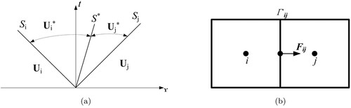
Several flux schemes have been designed to solve this kind of problem. However, many popular flux schemes cannot operate with a general fluid equation of state. For example, the Roe's flux scheme (Roe, 1981) and van Leer's (Van Leer, 1982) flux scheme, are derived under the ideal gas assumption, making use of ideal gas relations to reconstruct properties at the interface (Luo et al., 2004). Luo et al. (2004) studied three different schemes, AUSM+, HLLC and Godunov, with the Arbitrary Lagrangian–Eulerian (ALE) formulation for solving the unsteady compressible Euler equations. Numerical results indicate that HLLC ALE and Godunov schemes demonstrate robustness for solving such problems, while the AUSM+ ALE scheme exhibit strong oscillations at the interfaces (Luo et al., 2004). For NICFD problems, especially when using a LuT instead of an analytical equation of state, it is preferred to use a flux solver that is based on the interpolated properties on the left and right sides of the interface rather than having to reconstruct properties via a specific EoS at the interface. This ensures the flux calculator being agnostic of any assumptions relating to the equation of state. The HLLC ALE flux scheme provides such an ability (Luo et al., 2004). Flux across the interface between two adjacent cells is schematically shown in Figure 1(b). As the HLLC ALE flux scheme, for an ideal gas EoS is already available in OpenFOAM extend project 3.0 (Borm et al., 2011), and as it doesn't require reconstruction of interface conditions, the HLLC ALE flux scheme is selected for the current non-ideal gas solver. The HLLC ALE flux scheme is also more suitable for solving unsteady rotating turbomachinery problems, where moving grids are important (Luo et al., 2004). The following derivation of the HLLC ALE flux scheme is based on the unsteady compressible Euler equations for a moving control volume. Here the unsteady compressible Euler equations can be expressed in an integral form as (13) $\begin{array}{r}\frac{\mathrm{\partial }}{\mathrm{\partial }t}{\int }_{\mathrm{\Omega }\left(t\right)}\mathbf{U}\mathrm{d}\mathrm{\Omega }+{\int }_{\mathrm{\Gamma }\left(t\right)}\mathbf{F}\mathrm{d}\mathrm{\Gamma }=0\end{array}$(13) where $\mathrm{\Omega }\left(t\right)$ is the moving control volume and $\mathrm{\Gamma }\left(t\right)$ is its boundary, both varying with time (t). The flow variable vector U and inviscid flux vector F are defined by (14) $\begin{array}{r}\mathbf{U}=\left[\begin{array}{c}\rho \\ \rho \mathit{v}\\ \rho E\end{array}\right],\mathbf{F}=\left[\begin{array}{c}(\mathit{v}-\dot{\mathit{x}})\mathbf{\cdot }\mathit{n}\rho \\ (\mathit{v}-\dot{\mathit{x}})\mathbf{\cdot }\mathit{n}\rho \mathit{v}+p\mathit{n}\\ (\mathit{v}-\dot{\mathit{x}})\mathbf{\cdot }\mathit{n}\rho E+p\mathit{v}\mathbf{\cdot }\mathit{n}\end{array}\right]\end{array}$(14) where ρ, p, and E are the density, pressure, and specific total energy of the fluid, $\mathit{v}$ is the fluid velocity vector. $\mathit{n}$ denotes the unit outward normal vector to the moving boundary $\mathrm{\Gamma }\left(t\right)$, whose velocity is defined as $\dot{\mathit{x}}$ (Luo et al., 2004). Once the velocity of the moving boundary is set to zero, then the equations changed to stationary equations. This set of equations is completed by the addition of an equation of state which establishes the relationship between, at most, three thermodynamic variables. In the generic form, the equation of state is taken to be (15) $\begin{array}{r}\rho =\mathit{\rho }(e,p)\end{array}$(15) When using LuT method this becomes Equation (9(9) $\begin{array}{rl}\rho & ={\mathbf{L}}_{\rho }(e,p)\end{array}$(9) ). The specific internal energy, e, is related to the specific total energy by (16) $\begin{array}{r}e=E-\frac{|{\mathit{v}}^2|}{2}\end{array}$(16) To make the fluid properties conservative, the following geometric conservation law must be satisfied during grid motion and deformation. (17) $\begin{array}{r}\frac{\mathrm{\partial }\mathrm{\Omega }}{\mathrm{\partial }t}-{\int }_{\mathrm{\Gamma }\left(t\right)}\dot{\mathit{x}}\mathbf{\cdot }\mathit{n}\mathrm{d}\mathrm{\Gamma }=0\end{array}$(17) The geometric conservation law can be satisfied, either by explicitly updating the volume $\mathrm{\Omega }\left(t\right)$ through an evaluation of Equation (17(17) $\begin{array}{r}\frac{\mathrm{\partial }\mathrm{\Omega }}{\mathrm{\partial }t}-{\int }_{\mathrm{\Gamma }\left(t\right)}\dot{\mathit{x}}\mathbf{\cdot }\mathit{n}\mathrm{d}\mathrm{\Gamma }=0\end{array}$(17) ) or by implicitly defining the control surface area $\mathrm{\Gamma }\left(t\right)$ as a weighted average of the n and n + 1 time level areas, such that Equation (17(17) $\begin{array}{r}\frac{\mathrm{\partial }\mathrm{\Omega }}{\mathrm{\partial }t}-{\int }_{\mathrm{\Gamma }\left(t\right)}\dot{\mathit{x}}\mathbf{\cdot }\mathit{n}\mathrm{d}\mathrm{\Gamma }=0\end{array}$(17) ) is satisfied automatically by construction (Luo et al., 2004).

The solution of the Riemann problem in physical space is shown in Figure 1(a). The HLLC ALE flux calculator in this study follows the research of Batten et al. (1997). The fluxes are defined by (18) $\begin{array}{r}{\mathbf{F}}_{ij}^{\mathrm{H}\mathrm{L}\mathrm{L}\mathrm{C}}=\{\begin{array}{ll}{\mathbf{F}}_i,& \mathrm{i}\mathrm{f}{S}_i>0\\ \mathbf{F}\left({\mathbf{U}}_i^{\ast }\right),& \mathrm{i}\mathrm{f}{S}_i\le 0<S^{\ast }\\ \mathbf{F}\left({\mathbf{U}}_j^{\ast }\right),& \mathrm{i}\mathrm{f}{S}^{\ast }\le 0\le S_j\\ {\mathbf{F}}_j,& \mathrm{i}\mathrm{f}{S}_j<0\end{array}\end{array}$(18) where (19) $\begin{array}{rl}{\mathbf{U}}_K^{\ast }& =\left[\begin{array}{c}{\rho }_K^{\ast }\\ (\rho {\mathit{v}}_K{)}^{\ast }\\ (\rho E{)}_K^{\ast }\end{array}\right]\\ & =\frac{1}{S_K-S^{\ast }}\left[\begin{array}{c}(S_K-q_K){\rho }_K\\ (S_K-q_K)(\rho \mathit{v}{)}_K+(p^{\ast }-p_K)\mathit{n}\\ (S_K-q_K)(\rho E{)}_K-p_K{q}_K+p^{\ast }{S}^{\ast }\end{array}\right]\end{array}$(19) (20) $\begin{array}{rl}{\mathbf{F}}_K^{\ast }\equiv \mathbf{F}\left({\mathbf{U}}_K^{\ast }\right)& =\left[\begin{array}{c}{S}^{\ast }{\rho }_K^{\ast }\\ S^{\ast }(\rho \mathit{v}{)}_K^{\ast }+p^{\ast }\mathit{n}\\ S^{\ast }(\rho E{)}_K^{\ast }+(S^{\ast }+\dot{\mathit{x}}\mathbf{\cdot }\mathit{n})p^{\ast }\end{array}\right]\end{array}$(20) In these equations, i and j denote the left and right cell index, ${}^{\ast }$ denotes the value at the star region (the wedge region between $S_i$ and $S_j$, indicates the integral-averaged solution). K can be replaced by i and j to get the expressions for different variables, like ${\mathbf{U}}_i^{\ast }$, ${\mathbf{U}}_j^{\ast }$, etc. The normal relative speed q is calculated by (21) $\begin{array}{r}q=(\mathit{v}-\dot{\mathit{x}})\mathbf{\cdot }\mathit{n}\end{array}$(21) In the original version for the HLLC ALE flux calculator presented by Luo et al. (2004), the energy flux $\rho E$ is calculated: (22) $\begin{array}{r}\rho E=\frac{p}{\gamma -1}+\rho (\frac{1}{2}{\mathit{v}}^2+\mathrm{T}\mathrm{K}\mathrm{E})\end{array}$(22) where TKE is turbulent kinetic energy. For the new non-ideal implementation, the $\rho E$ flux calculation is changed to (23) $\begin{array}{r}\rho E=\rho h-p+\rho (\frac{1}{2}{\mathit{v}}^2+\mathrm{T}\mathrm{K}\mathrm{E})\end{array}$(23) using the fundamental relationship between E and h to negate the dependence on γ. The remaining variables are attained through an equation of state call (referring to the LuT, Equations (6(6) $\begin{array}{rl}h& ={\mathbf{L}}_h(e,p)\end{array}$(6) )–(9(9) $\begin{array}{rl}\rho & ={\mathbf{L}}_{\rho }(e,p)\end{array}$(9) ). The integral-averaged propagation speed in the star region ($S^{\ast }$) is calculated, (24) $\begin{array}{r}{S}^{\ast }=\frac{{\rho }_j\cdot q_j\cdot (S_j-q_j)-{\rho }_i\cdot q_i\cdot (S_i-q_i)+p_i-p_j}{{\rho }_j\cdot (S_j-q_j)-{\rho }_i\cdot (S_i-q_i)}\end{array}$(24) Here, the propagation speed on the left and right is calculated by (25) $\begin{array}{rl}{S}_i& =min(q_i-a_i,(\tilde{\mathit{v}}-\dot{\mathit{x}})\mathbf{\cdot }\mathbf{n}-\tilde{a})\end{array}$(25) (26) $\begin{array}{rl}{S}_j& =max(q_j+a_j,(\tilde{\mathit{v}}-\dot{\mathit{x}})\mathbf{\cdot }\mathbf{n}+\tilde{a})\end{array}$(26) with $\tilde{\mathit{v}}$ and $\tilde{a}$ being Roe's average variables for velocity and acoustic speed. $\tilde{\mathit{v}}$ and $\tilde{a}$ are calculated as (27) $\begin{array}{rl}\tilde{\mathit{v}}& =\frac{\sqrt{{\rho }_i}\cdot {\mathit{v}}_i+\sqrt{{\rho }_j}\cdot {\mathit{v}}_j}{\sqrt{{\rho }_i}+\sqrt{{\rho }_j}}\end{array}$(27) (28) $\begin{array}{rl}{\tilde{a}}^2& =\frac{\sqrt{{\rho }_i}\cdot a_i^2+\sqrt{{\rho }_j}\cdot a_j^2}{\sqrt{{\rho }_i}+\sqrt{{\rho }_j}}+{\eta }_{\gamma }\cdot (q_j-q_i{)}^2\end{array}$(28) with (29) $\begin{array}{r}{\eta }_{\gamma }=\frac{\gamma -1}{2}\frac{\sqrt{{\rho }_i}\sqrt{{\rho }_j}}{(\sqrt{{\rho }_i}+\sqrt{{\rho }_j}{)}^2}\end{array}$(29) and $a_i$ and $a_j$ are the local acoustic speed for the i and j side calculated by Equation (7(7) $\begin{array}{rl}a& ={\mathbf{L}}_a(e,p)\end{array}$(7) ). For most gases, the ratio of the specific heats γ is a constant between 1 and $5/3$, hence (30) $\begin{array}{r}{\eta }_{\gamma }<{\eta }_2=\frac{1}{2}\frac{\sqrt{{\rho }_i}\sqrt{{\rho }_j}}{(\sqrt{{\rho }_i}+\sqrt{{\rho }_j}{)}^2}\end{array}$(30) can be estimated.

In accordance with research by (Einfeldt, 1988), to extend to more general non-ideal fluid properties, ${\eta }_{\gamma }$ in Equation (29(29) $\begin{array}{r}{\eta }_{\gamma }=\frac{\gamma -1}{2}\frac{\sqrt{{\rho }_i}\sqrt{{\rho }_j}}{(\sqrt{{\rho }_i}+\sqrt{{\rho }_j}{)}^2}\end{array}$(29) ) is taken to be approximately ${\eta }_2$, which satisfies the stability requirements; interested readers may refer to the study by Einfeldt (1988). This step is very important, for it decouples the numerical dependence on calculating the specific heat ratio on the left and right cells, which allows using the more convenient LuT method. The integral-averaged pressure in the star region, $p^{\ast }$, is calculated as (31) $\begin{array}{rl}{p}^{\ast }& ={\rho }_i\cdot (q_i-S_i)\cdot (q_i-S^{\ast })+p_i\\ & ={\rho }_j\cdot (q_j-S_j)\cdot (q_j-S^{\ast })+p_j\end{array}$(31) The resulting HLLC flux calculator is found to have the following properties: (1) exact preservation of isolated contact and shear waves; (2) positivity-preserving of scalar quantities; and (3) enforcement of the entropy condition (Luo et al., 2004). This makes the flux calculator suitable for the current NICFD applications.

2.4. Real gas properties density based solver

In this section, the governing equations and workflow of the real gas properties density based solver RGDFoam are discussed. The newly developed solver for the OpenFOAM extend project is a derivative of the SIG turbomachinery DensityBasedTurbo solver, developed by Borm et al. (2011) and validated in studies by Borm and Kau (2012) and Reis (2013).

This solver is an approximate Riemann solver, with multiple flux calculator options. The implemented ALE formulation is rotating grid capable. Second-order spatial accuracy is reached as the interpolation for the inviscid terms is done with Van Leer's Monotonic Upstream-centered Schemes for Conservative Laws (MUSCL) (Van Leer, 1977). For acceleration, local and dual time stepping is implemented for steady and unsteady solutions, and Runge–Kutta time stepping is also available.

To solve turbulence in practice, the solver is implemented for the Navier–Stokes equations with Favre averaged quantities, using the Reynolds-Average Navier–Stokes (RANS) equations. The governing equations for a Favre averaged Navier–Stokes equation for rotating frames are (Borm et al., 2011) (32) $\begin{array}{rl}& \frac{\mathrm{\partial }\rho }{\mathrm{\partial }t}+\mathrm{\nabla }\mathbf{\cdot }\left(\rho {\mathit{v}}_{\mathrm{r}\mathrm{e}\mathrm{l}}\right)=0\end{array}$(32) (33) $\begin{array}{rl}& \frac{\mathrm{\partial }\rho \mathit{v}}{\mathrm{\partial }t}+\mathrm{\nabla }\mathbf{\cdot }(\rho {\mathit{v}}_{\mathrm{r}\mathrm{e}\mathrm{l}}\otimes \mathit{v})+\mathrm{\nabla }p=-\rho \left(\mathbf{\Omega }\times \mathit{v}\right)+\mathrm{\nabla }\mathbf{\cdot }\sigma \end{array}$(33) (34) $\begin{array}{rl}& \frac{\mathrm{\partial }\rho E}{\mathrm{\partial }t}+\mathrm{\nabla }\left(\right(\rho E+p){\mathit{v}}_{\mathrm{r}\mathrm{e}\mathrm{l}}+p{\mathit{v}}_{\mathrm{r}\mathrm{o}\mathrm{t}})=\mathrm{\nabla }\mathbf{\cdot }\left(\mathit{\sigma }\mathbf{\cdot }\mathit{v}\right)\\ & +\mathrm{\nabla }\mathbf{\cdot }\left(\lambda \mathrm{\nabla }T\right)+\mathrm{\nabla }\mathbf{\cdot }(\mu +{\mu }_T)\mathrm{\nabla }\mathrm{T}\mathrm{K}\mathrm{E}\end{array}$(34) Here, $\mathit{v}={\mathit{v}}_{\mathrm{r}\mathrm{e}\mathrm{l}}+{\mathit{v}}_{\mathrm{r}\mathrm{o}\mathrm{t}}$, where ${\mathit{v}}_{\mathrm{r}\mathrm{e}\mathrm{l}}$ is the relative velocity vector and ${\mathit{v}}_{\mathrm{r}\mathrm{o}\mathrm{t}}$ is the rotational speed of the reference frame, which is calculated by (35) $\begin{array}{r}{\mathit{v}}_{\mathrm{r}\mathrm{o}\mathrm{t}}=\mathbf{\Omega }\times \mathit{x}\end{array}$(35) TKE is the turbulent kinetic energy, and $\mathit{\sigma }$ is the total shear stress tensor, the sum of the laminar and turbulence shear stress tensors. The original implementation of the density based solver is based on the ideal gas equation of state. To create a density based solver, capable of solving the compressible non-ideal gas RANS equations, modifications are required, resulting in the new solver, RGDFoam, denoted as the Real Gas Density based Foam solver. The flow chart of the RGDFoam solver is provided in Figure 2.

Figure 2. Flow chart of the RGDFoam solver.

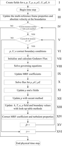
Compared with the original density based solver, RGDFoam is modified in the following steps. During step I, scalar fields for static internal energy, e, and acoustic speed, a, are created. In step VI, the pressure, p, field for the previous iteration is stored to allow usage of the waveTransmissive boundary condition with steady solutions. In step VII, the non-ideal HLLC ALE flux scheme discussed in Section 2.3 is initialized and solved. In step VIII, the pressure is solved with the secant method, described in Equation (11(11) $\begin{array}{r}{p}_{n-1}=(1+\delta )\cdot p_n\end{array}$(11) ). During step IX, the Multi-Reference Frame (MRF) coefficients are updated when simulating rotating machinery problems. In step XII, where pressure, enthalpy and acoustic speed are updated by a call to the equation of state, the call to the ideal gas equation is replaced by a call to the respective look-up-table function from Section 2.2. The resulting solver, RGDFoam, is capable of using LuTs to solve non-ideal compressible fluid dynamics problems. The source code for RGDFoam and the tabular data generator are available from the repository at https://github.com/cyjanry/RGDFoam_v1/ (Qi, 2017).

3. Validation and verification

To verify, validate and demonstrate the capabilities of the newly implemented real gas solver RGDFoam on solving steady-state NICFD Riemann problems for the stationary grid, this section presents the results for three reference cases taken from the literature.

First, RGDFoam is validated with experimental data for a transonic convergent–divergent nozzle operating with air, published by NASA (Hunter, 2004). This case is to show the accuracy of RGDFoam when simulating transonic flows and shock waves. Next, a cross-verification is presented, comparing RGDFoam results against the result from the NICFD solver SU2 (Economon et al., 2015) in a simulation of VKI turbine cascades with the dense gas MDM (Vitale et al., 2015). This case shows the ability to simulate non-ideal gas flows in a turbine relevant application. Finally, a 2D expansion corner case is set up for the dense gas ${\mathrm{M}\mathrm{D}}_4\mathrm{M}$. Here, analytical solutions are developed using the REFPROP database (Lemmon et al., 2013; Span & Wagner, 1996), and compared with the simulation results from RGDFoam. This explores the solver's ability to capture non-ideal fluid dynamics. One thing to be noted is that, in the present plan of development, the solver is only validated and verified on a stationary grid, which means that the rotational speeds are all set to zero for $\dot{\mathit{x}}$.

3.1. 2D simulation for NASA transonic air nozzle

This validation case consists of transonic air flowing through a convergent–divergent nozzle. Details of the geometry, experimental set up, and experimental data are presented in studies by Hunter (2004) and Abdol-Hamid et al. (2006). A grid dependency study was carried on with four meshes, 40 k, 60 k, 90 k and 135 k, as shown in Figure 3.

Figure 3. Grid dependency study for the NASA transonic air nozzle.

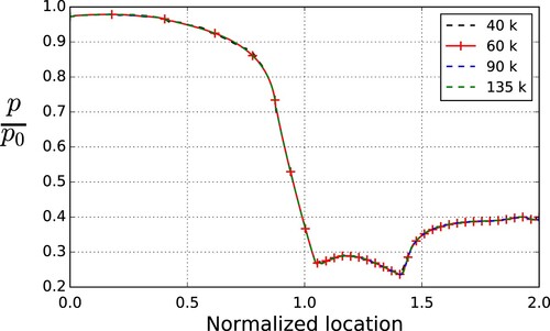
Results show that all of these meshes can return a good accuracy for the simulation. Hence, to keep a balance between accuracy and simulation speed, the mesh composed of 60 k is chosen to perform the calculations. To capture the complicated physics of the shock-boundary layer interaction process, the grid resolution of the divergent part of the CD nozzle is increased. The first cell height has a $y^{+}$ of approximately 0.5. To validate RGDFoam, four different simulations are performed to assess the effect of solver choice, turbulence model and equation of state implementation. The main parameters of the simulations are summarized in Table 1.

Table 1. Details for 2D simulation of NASA convergent–divergent air nozzle.

Items	Value
Solver	transonicMRFDyMFoam	transonicMRFDyMFoam	RGDFoam	RGDFoam
Case label	TR-0	TR-1	RGD-0	RGD-1
Fluid	Air
$T_{0\mathrm{i}\mathrm{n}}$ (K)	294.45
$p_{0\mathrm{i}\mathrm{n}}$ (Pa)	102,387.1
$p_o$ (Pa)	42,449.07
$C_p$ (J kg${}^{-1}$ K${}^{-1}$)	1006.88	1006.88	1006.88	LuT
μ (m${}^2$ s${}^{-1}$)	$1.8296\times {10}^{-5}$	$1.8296\times {10}^{-5}$	$1.8296\times {10}^{-5}$	LuT
γ (-)	1.4	1.4	1.4	LuT
Pressure ratio (-)	2.41
Gas model	Ideal gas	Ideal gas	LuT ideal gas	LuT real gas
Turbulent model	k–ω SST	k–ε	k–ω SST	k–ω SST
Turbulent intensity (%)	0.0375
Mixing length (m)	0.005
Spatial scheme	Gauss vanLeer
Flux scheme	HLLC ALE Flux		HLLC ALE Real Flux
Temporal scheme	EulerLocal
Local max CFL (-)	0.5

First, the simulations are carried out using the established turbomachinery solver transonicMRFDyMFoam (Borm et al., 2011; Reis, 2013). These simulations use the ideal gas EoS and are performed with two different turbulence models, k–ω SST and k–ε. The results are compared with the experimental data to show the influence of different turbulence models on the boundary layer separation position. Next, a simulation is carried out using RGDFoam using a look-up table generated using the ideal gas EoS (case RGD-0). This allows a direct comparison with transonicMRFDyMFoam (case TR-0) to verify the numerical implementation of the LuTs. Finally, the simulation is carried out using RGDFoam using an LuT based on non-ideal gas properties for air, taken from the REFPROP database (Lemmon et al., 2013, 2000). Comparing these four simulations with experimental data allows the implemented LuT formulation and solver to be validated. For the RGD-0 and RGD-1 simulations, LuTs with a resolution of $50\times 50$ (e, p) are used. When using linear interpolation, these tables introduce an error of less than 0.1% compared with the exact EoS, assessed using the method described in Appendix 2.

The results are presented in Figures 4 and 5. Figure 4 compares the normalized wall pressure ($p/p_0$) along the nozzle centerline obtained from experiments and predictions from the four different simulations.

Figure 4. Comparison of the wall centerline pressure between the ideal gas and real gas solvers, experimental data from Hunter (2004).

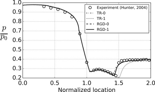
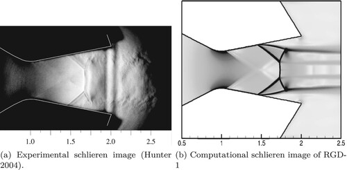
Figure 5. Comparison of experimental and computational schlieren images for the NPR 2.41 test case. (a) Experimental schlieren image (Hunter, 2004) and (b) Computational schlieren image of RGD-1.

The comparison between experimental data and simulation cases TR-0 and TR-1 from Figure 4 shows that the k–ω SST turbulent model has better performance capturing the location of boundary layer separation. The k–ε model matches the k–ω SST model in the upstream region, and far downstream of the separation location. However, based on the experimental data, the k–ε model predicts a delayed boundary layer separation. This is consistent with the literature, which reports that the ε equation overpredicts the turbulent length scale in flows with adverse pressure gradients, resulting in high wall shear stress and overprediction of separation length (Menter & Esch, 2001).

As the k–ω SST model includes a better near-wall treatment, it is more capable of predicting the separation for regions with adverse pressure gradients, as demonstrated in this case. The k–ω SST model is used for subsequent simulations with RGDFoam.

When comparing the experimental data with simulation cases TR-0 and RGD-0, it is observed that both are in close agreement with the experimental data for nozzle centerline pressure and that there is only a marginal difference between the two predictions. Both simulations have the same pressure magnitudes; however, there is a small difference in separation location. As both simulations use the same EoS (once by direct evaluation and once through the LuT), the same turbulence model and the same flux calculators, this demonstrates the appropriate implementation and operation of RGDFoam.

The data lines for simulation cases RGD-0 and RGD-1, corresponding to ideal gas and real gas LuTs, are generally indistinguishable. This is because the conditions are far away from the critical point of air (405.56 K, 3.77 MPa). Thus, in the fluid properties from the LuT, the captured actual gas properties are more or less identical with the ideal gas properties.

Figure 5(a) presents the experimental schlieren image presented by Hunter (2004) for a pressure ratio of 2.41. It can be seen that the airflow is fully detached at the top and bottom wall, and that a well-defined lambda foot and Mach disk are formed at a position of approximately $x/x_t=1.70$. Before the Mach disk, two oblique shocks are originating from the walls, which connect the walls and the Mach disk. The shock detachment from the side walls happens near $x/x_t=1.45$. Fully turbulent flow exists after the shock boundary layer detachment, resulting in a long turbulent jet plume after the lambda foot. Figure 5(b) is a computational schlieren like image that shows the spatial density gradient obtained from the results of RGDFoam, RGD-1, simulated with non-ideal gas look-up tables. Inspection of the images illustrates that the numerical results are in excellent agreement with the experimental data, such as the shock detachment points and oblique shock angles. The shock detachment locations are as seen in Figure 4, and the Mach disk position has shifted slightly compared with the experimental result. This is most likely caused by backflow from the outlet corner, the angle of which is uncertain and different between the schematic diagram in the study (Hunter, 2004) and their schlieren image, reproduced in Figure 5(a). For the current simulations, an angle of ${69.41}^{\circ }$ is used. The comparison between Figure 5(b) and Abdol-Hamid's study (Abdol-Hamid et al., 2006, Figure 10) shows excellent agreement.

3.2. VKI 2D stator cascade

The second case tests the ability of RGDFoam to predict the flow of a dense organic fluid (non-ideal gas) through the VKI LS-89 turbine stator cascade (Arts et al., 1990). The case uses thermodynamic inlet conditions close to the critical point, previously analysed by Vitale et al. (2015) using SU2, to demonstrate the ability of the solver to work with non-ideal gas properties. The working fluid belongs to the ${\mathrm{M}\mathrm{D}}_n\mathrm{M}$ class and is among the non-ideal fluids, commonly used in ORCs (Maraver et al., 2014).

In the absence of high-quality experimental data for validation of non-ideal flows, a cross-verification between Stanford Unstructured 2 (SU2) and OpenFOAM is conducted to show that RGDFoam can capture the non-ideal flow properties correctly. SU2 is a well-established open-source platform for solving multi-physics PDE problems on general unstructured meshes, with a RANS solver capable of simulating turbulent compressible flows typical of aerospace engineering problems (Economon et al., 2015; Palacios et al., 2013). SU2 has recently been extended to NICFD simulation, and cross-verified with a range of different solvers (Vitale et al., 2015), and has recently been validated through comparison with experiments from TROVA (Gori et al., 2017). Different equations of state are implemented in SU2 to perform NICFD simulations. The case studied by Vitale et al. (2015) uses the PR equation of state (see Appendix 1), together with a constant ratio of heat capacity and constant dynamic viscosity, leading to a pseudo-real gas simulation.

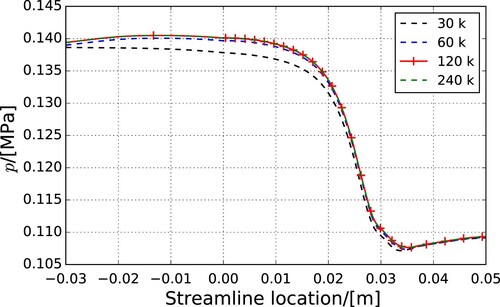
For the cross-verification, two RGDFoam simulations are conducted. Agrid dependency study was carried out with four resolutions of grid, 30 k, 60 k, 120 k and 240 k, as shown in Figure 6. Obviously, the 120 k mesh will return a good balance between accuracy and simulation speed. Thus, the 120 k mesh is chosen to perform the calculations. The first, OF-1, mimics the pseudo-real gas implementation from SU2 to allow a direct comparison. The second, OF-2, uses fully non-ideal fluid properties, with look-up table values developed from the REFPROP database (Colonna et al., 2008; Lemmon et al., 2013). This case shows the influence of varying viscosity and heat capacity on fluid dynamics. A detailed case description is available in the study by Vitale et al. (2015). The simulation settings, fluid properties and boundary conditions are listed in Table 2. It is to be noted that there are few differences between the meshes used for OpenFOAM and SU2. The periodic boundaries for OpenFOAM were extracted by the location of nozzle centerlines. It is worth noting that the turbine cascade operation conditions are selected to be near the critical point to promote strong non-ideal fluid dynamic behavior. The compressibility factor for MDM in the simulation is between 0.601 and 0.777. The three different simulation cases are marked as SU2, OF-1 and OF-2, respectively. A comparison of temperature, pressure, density and Mach number along a streamline following the cascades channel is shown in Figure 7, and Mach number contours are shown in Figure 8, with the SU2 data obtained from Vitale et al. (2015).

Figure 6. Grid dependency study for the VKI turbine case.

A limitation of the SU2 data is that the exact location of the streamline used by the authors for data extraction is not provided. In the current work, the channel centerline is picked for data comparison. Figure 7 shows that the OF-1 case has very good agreement with the SU2 simulation before x = 0.025 for all properties. In this region, the spatial property gradients normal to the channel centerline are small, meaning that the uncertainty in the location of data extraction only has a minor impact. As such, this confirms that the OF-1 simulation can correctly reproduce the results from SU2. However, after x = 0.025, the data lines separate. This location corresponds to the nozzle exit area where large spatial property gradients exist. Furthermore, the two simulations use different turbulence models. In SU2, the Spalart–Allmaras (SA) one-equation turbulence model is chosen to close the momentum equation, whereas in OpenFOAM, the k–ω SST turbulence model is selected. These models result in different boundary layers, and turbulence and entropy wakes forming at the stator (or airfoil) trailing edge. These different wakes manifest as the variations in properties seen in Figure 7 and also visible in Figure 8.

Figure 7. Comparison of fluid properties along streamline at near mid-passage in VKI cascade. (a) Temperature. (b) Pressure. (c) Density and (d) Mach number.

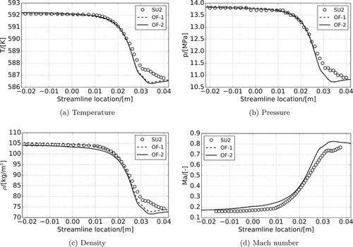
Figure 8. Comparison of SU2 and OF-2 Mach number contours of the VKI LS89 turbine stator cascades. (a) Case SU2, carried out by SU2 with the Peng–Robinson equation of state and (b) Case OF-2, carried out by RGDFoam with REFPROP based look-up tables.

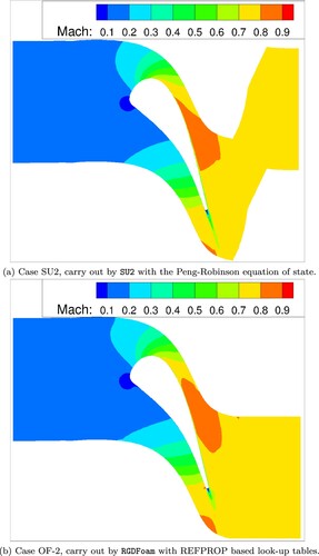
Table 2. Details for 2D simulation of VKI stator cascade.

Items	Values
Solver	SU2 (Peng–Robinson)	OpenFOAM (Peng–Robinson)	OpenFOAM REFPROP
Case label	SU2	OF-1	OF-2
Number of cells (-)	16,000	125,516	125,516
Fluid	MDM
$T_{\mathrm{c}\mathrm{r}}$ (K)	564.1
$p_{\mathrm{c}\mathrm{r}}$ (Pa)	$1.415\times {10}^6$
Acentric factor (-)	0.529
R (J kg${}^{-1}$ K${}^{-1}$)	35.23
$T_{0\mathrm{i}\mathrm{n}}$ (K)	592.1
$p_{0\mathrm{i}\mathrm{n}}$ (Pa)	1.387$\times {10}^6$
$p_o$ (Pa)	1.10$\times {10}^6$
Gas model	Peng–Robinson	Peng–Robinson based look-up table	REFPROP based look-up table
Cp (J kg${}^{-1}$ K${}^{-1}$)	2170.38	2170.38	REFPROP based look-up table
Cv (J kg${}^{-1}$ K${}^{-1}$)	2135.15	2135.15	REFPROP based look-up table
γ (-)	1.0165	1.0165	REFPROP based look-up table
μ (m${}^2$ s${}^{-1}$)	1.3764$\times {10}^{-5}$	1.3764$\times {10}^{-5}$	REFPROP based look-up table
Spatial scheme	Gauss vanLeer
Temporal scheme	EulerLocal
Flux scheme	Roe	HLLC ALE Real Flux
Spatial accuracy	2nd order
Turbulence model	Spalart–Allmaras	k–ω SST	k–ω SST
Local max CFL (-)	5.0	0.8	0.8

The predicted properties converge again at the downstream end of the simulation domain, confirming that this is a localized effect. Overall, apart from the turbulent wake, good agreement exists between the SU2 and OF-1 simulations, confirming the ability of RGDFoam to simulate non-ideal gas flows correctly in turbine stationary cascades.

In the OF-2 simulation, fully non-ideal gas properties are used. It can be seen from Figure 7 that the predicted pressure and Mach number are close among different approaches, but there is an offset in pressure, temperature and density from the outset. This is due to the differences in the equations of state. A further reason is the non-constant fluid viscosity that is applied via the look-up table method. The deviations in the wake (x>0.025), where turbulent viscosity has an important influence on temperature and density, highlights the importance of correct non-ideal gas modelling.

As there is no obvious difference in Mach number between OF-1 and OF-2, the Mach number contour for the SU2 and OF-2 cases are shown in Figure 8. This figure shows good agreement upstream of the wake region. However, the SU2 case has a longer low-velocity wake (low Mach number) than the OF-2 case, which can be attributed to the different turbulence models.

3.3. Dense gas flow over a 2D backward ramp

3.3.1. Theory of non-ideal gas region

At thermodynamic conditions close to the critical point, some dense gases exhibit non-ideal behavior. Cramer published a detailed study of the non-ideal dynamics of gases (Cramer, 1991), unveiling new phenomena including the formation and propagation of expansion shocks, sonic shocks, double sonic shocks and shock splitting, and gave an analytical solution for these new phenomena. Cramer and Crickenberger (1992) studied the relationship between the Prandtl–Meyer function and Mach numbers for dense gases, and gave an estimation of the non-ideal behavior for the Prandtl–Meyer function. The expansion shock has been reviewed and studied by Thompson and Lambrakis (1973).

When discussing non-ideal behavior, the fundamental derivative, Γ, is used to determine whether the fluid properties enter the non-ideal gas region (Thompson, 1971). The fundamental derivative Γ is given by (36) $\begin{array}{rl}\mathrm{\Gamma }& =\frac{a^4}{2v^3}{\left(\frac{{\mathrm{\partial }}^{2}v}{\mathrm{\partial }{p}^2}\right)}_s\\ & =1+\frac{\rho }{a}{\left(\frac{\mathrm{\partial }a}{\mathrm{\partial }\rho }\right)}_s\end{array}$(36) where v denotes the specific volume, and acoustic speed is given by: (37) $\begin{array}{r}a={\left(\frac{\mathrm{\partial }p}{\mathrm{\partial }\rho }\right)}_s^{1/2}\end{array}$(37) Based on the study of Thompson (1971), the behavior of fluid properties along an isentrope for various values of Γ is shown in Table 3.

Table 3. Behavior of fluid properties along an isentrope for various values of Γ (Thompson, 1971).

Γ	Behavior
$\mathrm{\Gamma }>1$	Acoustic speed increases with pressure—behavior of usual substances
$\mathrm{\Gamma }=1$	Constant acoustic speed, pressure is a linear function of ρ
$0<\mathrm{\Gamma }<1$	Acoustic speed decreases with pressure
$\mathrm{\Gamma }=0$	Pressure is a linear function of $1/\rho$
$\mathrm{\Gamma }<0$	Negative curvature of isentrope—behavior of unusual substances

For a perfect gas ($pv=RT$), it can be shown that (38) $\begin{array}{r}\mathrm{\Gamma }=\frac{\gamma +1}{2}\end{array}$(38) Obviously, (39) $\begin{array}{r}\mathrm{\Gamma }>1\mathrm{i}\mathrm{f}\gamma >1\end{array}$(39) Hence, for perfect gases, a increases with ρ and p along an isentrope (Cramer & Crickenberger, 1992). For air, steam or ${\mathrm{C}\mathrm{O}}_2$, the value of Γ is greater than one, meaning that a increases in compression and decreases through an expansion (Durá Galiana et al., 2016). However, for organic fluids with high molecular complexity, the fundamental derivative, Γ, close to the critical point can drop below one or zero (Colonna et al., 2009). For isentropic processes, as Γ reduces, the rate of change of a with ρ decreases, and for $\mathrm{\Gamma }<1$, a decreases with p. The effect of Γ on the Prandtl–Meyer function ν is discussed by Thompson (1971) and Durá Galiana et al. (2016). They show that, for certain conditions with $\mathrm{\Gamma }<1$, a increases through an expansion, leading to the possibility of a rarefaction shock.

Thompson (1971) has shown that the region of inverted gas dynamics is defined by $M^2>1/(1-\mathrm{\Gamma })$. Here, the Mach number decreases with increasing flow velocity in a steady isentropic expansion. Thus, a region of non-ideal behavior delimited by J>0 is introduced, where J is defined by the following relationship between Γ and M: (40) $\begin{array}{r}J=-\frac{\nu }{M}\left(\frac{\mathrm{d}M}{\mathrm{d}\nu }\right)=1-\mathrm{\Gamma }-\frac{1}{M^2}\end{array}$(40) For certain conditions and thermodynamic models, gas can enter this non-ideal region. In this region, classical gas dynamics are inverted, meaning that M decreases through expansion waves as the Prandtl–Meyer function (ν) is inverted.

This phenomenon has attracted attention from researchers working on ORC design. Some dense gases, considered as an ideal working fluid for ORCs, such as $R245fa$ and ${\mathrm{M}\mathrm{D}}_n\mathrm{M}$, exhibit this non-ideal region (Chen et al., 2010; Durá Galiana et al., 2016). Thus it is important for a non-ideal gas CFD solver to simulate the fluid dynamics accurately when fluid properties are in this particular region. Vitale et al. (2015) performed a numerical study to capture one of the non-ideal gas dynamics phenomena, expansion shock, during verification of the NICFD solver SU2. For their case, the value of the fundamental derivative, Γ, is less than zero. Durá Galiana et al. (2016) performed a numerical study to show that dense gas properties can enter the non-ideal region through an isentropic expansion from given stagnation conditions. In such an expansion, the Mach number first increases but then decreases, while the fundamental derivative (Γ) first decreases to near zero before increasing again to near one. Thus there is a maximum M during the isentropic expansion, and the non-ideal gas dynamics for $0<\mathrm{\Gamma }<1$ can be captured. As the expansion process is isentropic and M>1, properties along a streamline are described by the analytical solution of an isentropic process. This process is analogous to the work for SU2 by Vitale et al. (2015).

3.3.2. Simulation case description

Investigating a similar case and comparing RGDFoam predictions with the analytical solution is a further way to assess the capability of RGDFoam and especially to assess the operation of the non-ideal gas LuTs in this non-ideal gas region. The fluid considered is ${\mathrm{M}\mathrm{D}}_4\mathrm{M}$, with critical properties of $T_{\mathrm{c}\mathrm{r}}=653.2K$ and $P_{\mathrm{c}\mathrm{r}}=0.877MPa$. An isentropic expansion routine is designed to determine the analytical solution for the non-ideal expansion process. To ensure that the fluid properties enter the non-ideal region through expansion, the stagnation temperature and pressure are chosen based on the study by Durá Galiana et al. (2016) to be $T_0=1.025T_{\mathrm{c}\mathrm{r}}$ and $p_0=2.0P_{\mathrm{c}\mathrm{r}}$. A pressure, $p=0.001P_{\mathrm{c}\mathrm{r}}$ is applied as the outlet. The analytical solution for the properties along this isentropic expansion process is calculated using properties obtained from the National Institute of Standards and Technology (NIST) real gas database (REFPROP) (Colonna et al., 2008; Lemmon et al., 2013). Using the isentropic assumption, M, T, p, Γ and ν for each point along a streamline through the expansion are evaluated.

Four grids have been chosen for the grid dependency study, with resolutions of 28 k, 48 k, 75 k and 131 k. The result is shown in Figure 9.Even though the 48 k grid can return a grid-independent result, considering that this case is used to validate the solver with an analytical simulation, the highest resolution of grid 131 k is chosen to carry out the following simulations.

Figure 9. Grid dependency study for the 2D backward ramp.

Figure 10 shows values of p, T, Γ and the value of ν versus local M along the isentropic expansion process. It can be seen that, at the beginning of the expansion, the local M increases as p and T decrease (Figures 10(a) and 10(b)). However, once the expansion enters the non-ideal region, M starts to decrease again. Thus, a maximum local M of 1.962 is reached.

Figure 10. Changing properties as a function of M for an isentropic expansion of ${\mathrm{M}\mathrm{D}}_4\mathrm{M}$. (a) p. (b) T. (c) Γ and (d) ν.

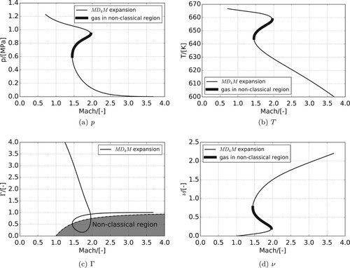
Figure 10(c) shows the non-ideal region, based on J>0. The peak in Mach number coincides with the fluid properties entering the non-ideal region. While J>0, M decreases until properties exit the non-ideal region. Once the gas properties are outside of the non-ideal region, M increases again.

For validation of the CFD solver RGDFoam, the fluid dynamics near the local peak in M are of interest. Thus, a test case that allows the fluid to expand from the classical region into the non-ideal region is designed. For this, a backward ramp with angle ${30}^{\circ }$ is selected to expand and accelerate the fluid. Owing to its relative simplicity, the 2D backward ramp is one of the most popular geometries used to evaluate CFD problems. For example, Vitale et al. (2015) use the backward step to capture a rarefaction shock-wave. The simulation details are listed in Table 4.

Table 4. Simulation details for expansion from the classical into the non-ideal region over a 2D backward ramp.

Items	Values
Solver	RGDFoam
Cell number	139,400
Fluid	MD${}_4$M
$T_{\mathrm{c}\mathrm{r}}$	653.2 K
$p_{\mathrm{c}\mathrm{r}}$	$0.877\times {10}^6$ Pa
$T_{0\mathrm{i}\mathrm{n}}$	$1.025T_{\mathrm{c}\mathrm{r}}$
$p_{0\mathrm{i}\mathrm{n}}$	$2.0p_{\mathrm{c}\mathrm{r}}$
$U_{\mathrm{i}\mathrm{n}}$	$\mathrm{M}\mathrm{a}\mathrm{c}\mathrm{h}=1.8$
Gas model	REFPROP based LuT
Spatial scheme	Gauss vanLeer
Temporal scheme	EulerLocal
Flux scheme	HLLCALE Real Flux
Viscosity model	inviscid
Spatial accuracy	2nd order

Contours of M, p, T and ρ are plotted in Figure 11 and corresponding properties along two streamlines are shown in Figure 12. Fluid enters the domain with a constant M, 1.8, which accelarated through an isentropic process from the staganation condition. Once the fluid reaches the Mach waves originating from the corner, the fluid starts to accelerate. The M first increases, while still in the classical region (J<0), forming an expansion fan. However once the fluid properties enter the non-ideal region (J>0), M starts to reduce, signifying a non-ideal process.

Figure 11. Contours for gas properties of the 2D simulation for dense gas flow passing a backward ramp. (a) Changes in M through isentropic expansion. (b) Changes in p through isentropic expansion. (c) Changes in T through isentropic expansion and (d) Changes in ρ through isentropic expansion.

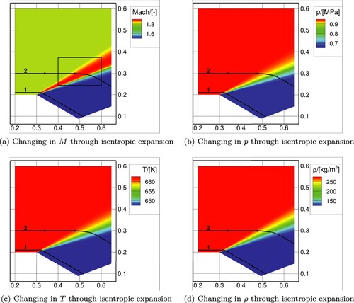
Figure 12. Changes in M through isentropic expansion, corresponding to Figures 10 and 11. (a) M along streamline 1. (b) M along streamline 2. (c) p against M along streamline 1. (d) p against M along streamline 2. (e) T against M along streamline 1 and (f) T against M along streamline 2.

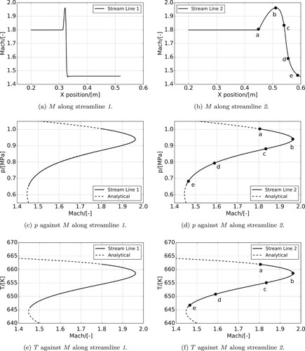
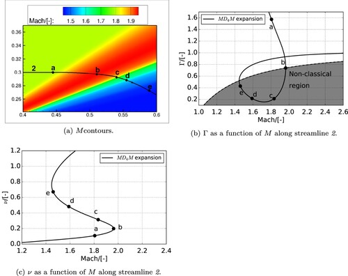
To gain a better understanding of this phenomenon, two streamlines are selected from the calculation domain, marked ‘1’ and ‘2’. Properties along these streamlines are shown in Figure 12. A close-up view of the M contours along streamline 2, during the expansion process, marked with a rectangular frame in Figure 11(a), is shown in Figure 13(a). Corresponding relationships between Γ and ν, and M are shown in Figures 13(b) and 13(c). Five markers, as positioned in Figure 13, have been added to allow a better description of the expansion process.

Figure 13. Close-up views of MD${}_4$M expansion routines along streamline 2 with markers to identify key steps in the process. (a) Mcontours. (b) Γ as a function of M along streamline 2. and (c) ν as a function of M along streamline 2.

Figures 12(a) and 12(b) show M along the x-position for streamlines 1 and 2, respectively. It is clear from Figure 12(a) that M gradually increases once the fluid starts to turn. For streamline 1, a maximum M is reached at x = 0.32. After this point, the streamlines enter the non-ideal region and M starts to drop.

Once the streamline is parallel with the second wall, M is constant again and equal to 1.46. Comparing streamlines 1 and 2, it can be seen that the expansion process is more spaced out, owing to the increased distance from the corner. The maximum and minimum M remain the same, 1.96 and 1.46, respectively.

It can be seen from Figures 12(b) and 13(a) that M increases from point a to point b. An expansion fan is formed, as the fluid accelerates and approaches the non-ideal region. Point b marks the position where the maximum M is reached and also the start of the non-ideal flow, as shown in Figure 13. As properties enter the non-ideal region, M starts to decrease.

Considering Figure 12(b), the most rapid reduction in M exists between points c and d. Here, the spatial rate of change of M, $\mathrm{\partial }M/\mathrm{\partial }x$, is highest for the entire process between points b and e. The region c to d also corresponds to the lowest Γ, as shown in Figure 13(b). This is explained by the local ratio of ν to M ($\mathrm{\Delta }\nu /\mathrm{\Delta }M$). Using data obtained from Figure 13(c) the values of $\mathrm{\Delta }\nu /\mathrm{\Delta }M$ for bc, cd and de are −0.90, −0.69 and −1.46, respectively. Thus, in region cd, the most rapid M decrease per unit turning angle is obtained. For fluids or conditions that result in a lower Γ, this could lead to the formation of a rarefaction shock.

Figures 12(c)–12(f) show the variation of p and T for both the analytical solutions and CFD simulations obtained using RGDFoam along the streamlines. It is clear that the pressure and temperature changes against M along both streamlines 1 and 2 (bold lines) show good agreement with the analytical solutions obtained from the ${\mathrm{M}\mathrm{D}}_4\mathrm{M}$ expansion routine (dashed lines). The implemented look-up tables, HLLC ALE flux calculator, and RGDFoam solver as a whole can recreate the analytical solutions accurately. This further demonstrates the ability of RGDFoam to perform predictions for dense gases with operating conditions close to the critical point and in the non-ideal gas region. The close agreement between the NICFD simulation results and the analytical solutions, obtained by direct evaluation of the REFPROP fluid property database, further confirms that using the LuTs with appropriate resolution does not introduce an appreciable error.

4. Conclusions

This article describes an extension of the open-source CFD library OpenFOAM (version 3.0 ex) to perform Reynolds averaged Navier–Stokes simulations of trans-sonic compressible flows of non-ideal fluids. The new solver, RGDFoam, using look-up tables to update non-ideal gas physical properties and transport properties, together with an appropriate Riemann flux calculator, are developed, verified and validated. The newly developed solver with the proposed flux calculator is efficient and flexible to various forms of equation of state, either analytic or tabulated. It is suitable for the simulation of non-ideal compressible fluid dynamics (NICFD) problems.

Three test cases are used to validate and verify the RGDFoam solver. First, a test case published by NASA, consisting of transonic under-expanded airflow through a convergent–divergent nozzle, is simulated. This confirms the ability of RGDFoam to simulate transonic flow phenomena and shock waves correctly. Secondly, a VKI 2D cascade operating with dense gas belonging to the ${\mathrm{M}\mathrm{D}}_n\mathrm{M}$ family in conditions near the critical point is simulated (compressibility factor between 0.601 and 0.777). This shows that the look-up tables and RGDFoam can correctly simulate non-ideal gas flows in near sonic stator geometries. Finally, the flow of ${\mathrm{M}\mathrm{D}}_4\mathrm{M}$ over a 2D backward ramp, in conditions that result in non-ideal effects, are simulated and compared with analytical conditions. This further verifies the abilities of RGDFoam to simulate non-ideal gas dynamics.

However, there are a few limitations of this study that need to be addressed in continued development in future, such as the following.

• The ability to solve rotating grid or multi-reference-frame problems, which will be a benefit for the whole of turbomachinery simulation.

• The ability to solve unsteady flows, which will help to understand time-dependent flow characteristics.

• The ability to treat 3D complicated geometries, which allows this solver more flexibility in engineering applications.

In conclusion, a new solver, RGDFoam, has been presented that is suitable for solving NICFD problems for OpenFOAM.

Nomenclature

CD	=	Convergent-Divergent.
CFD	=	Computational Fluid Dynamics.
CFL	=	Courant-Friedrichs-Lewy condition.
EoS	=	Equation of State.
LuT	=	Look-up Table.
MD${}_4$M	=	${\mathrm{C}}_{14}{\mathrm{H}}_{42}{\mathrm{O}}_5{\mathrm{S}\mathrm{i}}_6$, Tetradecamethylhexasiloxane.
MDM	=	${\mathrm{C}}_8{\mathrm{H}}_{24}{\mathrm{O}}_2{\mathrm{S}\mathrm{i}}_3$, Octamethyltrisiloxane.
MRF	=	Multi-reference frame.
NICFD	=	Non-ideal compressible flow dynamics.
PR	=	Peng–Robinson Equation of State.
TKE	=	Turbulence kinetic energy.
$\mathit{\sigma }$	=	Total shear stress tensor.
$\mathbf{\Omega }$	=	Angular speed vector.
δ	=	A small increment in number.
Γ	=	The fundamental derivative.
γ	=	Heat capacity ratio.
${\mathrm{\Gamma }}_{\left(t\right)}$	=	The boundary of the moving control volume.
μ	=	Dynamic viscosity [kg m${}^{-1}$ s${}^{-1}$].
ν	=	Kinematic viscosity [m${}^2$ s${}^{-1}$]; The Prandtl–Meyer function.
ω	=	Gas acentric factor.
${\mathrm{\Omega }}_{\left(t\right)}$	=	Moving control volume.
Φ	=	All other state properties.
ϕ	=	Specific state property.
ρ	=	Density [kg m${}^{-3}$].
$\mathit{n}$	=	The unit outward normal vector to the boundary.
$\mathit{v}$	=	Velocity vector.
$\dot{\mathit{x}}$	=	Velocity vector of the moving domain.
$\tilde{a}$	=	Roe's average for acoustic speed [m s${}^{-1}$].
$\tilde{v}$	=	Roe's average for velocity [m s${}^{-1}$].
a	=	Acoustic speed [m s${}^{-1}$].
$C_p$	=	Constant pressure specific heat capacity [J kg${}^{-1}$ K${}^{-1}$].
$C_v$	=	Constant volume specific heat capacity [J kg${}^{-1}$ K${}^{-1}$].
E	=	Specific total energy [J kg${}^{-1}$].
e	=	Internal energy [J kg${}^{-1}$].
h	=	Specific enthalpy[kJ K${}^{-1}$]
M	=	Mach number (-).
p	=	Pressure [Pa].
q	=	The normal relative speed [m s${}^{-1}$].
R	=	Gas constant [J kg${}^{-1}$ K${}^{-1}$].
S	=	Speed of the propagation of the shock, [m s${}^{-1}$].
T	=	Temperature, [K].
v	=	The specific volume, [m${}^3$ kg${}^{-1}$]
F	=	Inviscid flux vector.
L	=	The look-up functions.
U	=	The flow variable vector
*	=	Integral-average solution.
0	=	Total condition.
cr	=	Critical condition.
i	=	The ith or left cell/element.
in	=	Properties on inlet section.
j	=	The jth or right cell/element.
o	=	Properties on outlet section.
rel	=	Relative condition.
rot	=	Rotational condition.
x	=	Index number, can be replaced by i or j.

Acknowledgments

The research reported herein was begun at the University of Queensland, Australia, as part of the Australian Solar Thermal Research Initiative (ASTRI), a project supported by the Australian Government through the Australian Renewable Energy Agency, then continued at Shandong University and North China Electric Power University. The authors finalized the main body of this research. Many thanks are also due to Dr Ingo H.J. Jahn for his supervision on my PhD study. Vielen Dank an Dr. Ingo H. J. Jahn für die Hilfe und Unterstützung meiner Doktorarbeit. The authors also thank former members of the Queensland Geothermal Energy Centre for Excellence (QGECE) who granted access to various codes. NASA is acknowledged as the source of Figure 5(a) (The NASA Langley Research Center). Thanks also go to Mr Minggang Jiang for his assistance with debugging, and to the anonymous reviewers, whose great help turned the manuscript into its final shape.

Data availability statement

The source code of RGDFoam and the separate tabular data generator are available in the repository of Qi (2017).

Disclosure statement

No potential conflict of interest was reported by the author(s).

Additional information

Funding

The authors would like to thank the following funding bodies for their financial support: the National Natural Science Foundation of China [Grant Nos 52106049, 52130608]; the Natural Science Foundation of Shandong Province [Grant No. ZR2020QE191]; the Natural Science Foundation of Jiangsu Province [Grant No. BK20210113]; the Young Scholars Program of Shandong University [Grant No. 31380089964175]; the China Scholarship Council [Grant No. 201406220150].

Appendices

Appendix 1. Peng–Robinson equation of state

Peng–Robinson proposed their non-ideal gas model in 1976. The model modifies the Soaveâ–Redlichâ–Kwong (SRK) equation of state to improve the prediction of fluid density, vapour pressures and equilibrium ratios. The polytropic Peng–Robinson model can be conveniently written as (Vitale et al., 2015): (A1) $\begin{array}{rl}p(T,v)& =\frac{RT}{v-b}-\frac{a{\alpha }^2\left(T\right)}{v^2+2bv-b^2}\end{array}$(A1) (A2) $\begin{array}{rl}e(T,v)& =c_{v}T-\frac{a\alpha \left(T\right)(k+1)}{b\sqrt{2}}{\tanh }^{-1}\left(\frac{b\sqrt{2}}{v+b}\right)\end{array}$(A2) (A3) $\begin{array}{rl}s(T,v)& =c_v\ln \left(T\right)+R\ln (v-b)\\ & -\frac{a\alpha \left(T\right)(k+1)}{b\sqrt{2T{T}_{\mathrm{c}\mathrm{r}}}}{\tanh }^{-1}\left(\frac{b\sqrt{2}}{v+b}\right)\end{array}$(A3) The definition of the respective constants can be found in Vitale et al. (2015). Here, the $\alpha \left(T\right)$ represents the inter-molecular attraction force, which depends on temperature, T, while a and b are usually treated as temperature independent. Their values are calculated as follows: (A4) $\begin{array}{rl}a& =0.45725\frac{(R{T}_{\mathrm{c}\mathrm{r}}{)}^2}{p_{\mathrm{c}\mathrm{r}}}\end{array}$(A4) (A5) $\begin{array}{rl}b& =0.0778\frac{R{T}_{\mathrm{c}\mathrm{r}}}{p_{\mathrm{c}\mathrm{r}}}\end{array}$(A5) (A6) $\begin{array}{rl}\alpha (T,\omega )& =1+k(1-\sqrt{\frac{T}{T_{\mathrm{c}\mathrm{r}}}})\end{array}$(A6) k can be determined by (A7) $\begin{array}{r}k=\{\begin{array}{ll}0.37464+1.54226\omega -0.26992{\omega }^2& \omega \le 0.49\\ 0.379642+1.48503\omega \\ -0.164423{\omega }^2+0.016666{\omega }^3& \omega >0.49\end{array}\end{array}$(A7) The static enthalpy (h) used in the reconstruction of temperature is defined as (A8) $\begin{array}{r}h=e+\frac{p}{\rho }\end{array}$(A8) Thus, the first derivative of h is calculated as (A9) $\begin{array}{r}{\left(\frac{\mathrm{\partial }h}{\mathrm{\partial }T}\right)}_{\rho }=\frac{R}{\gamma -1}+\frac{ak(k+1)}{2b\sqrt{2T{T}_{\mathrm{c}\mathrm{r}}}}{\tanh }^{-1}\frac{b\sqrt{2}}{v+b}\end{array}$(A9)

Appendix 2.

Appendix 2. Tools for tabular data generation, comparison and error estimation

This section describes a Tabular Data Comparison and Error Estimation (TDCEE) utility to support non-ideal CFD simulations. A key feature of the tool is to estimate the accuracy of tables used in non-ideal CFD simulations. This is obtained from a comparison between tabular values and the real gas properties database. With the help of this tool, a look-up table with a smaller size can offer enough accuracy (the error is lower than 0.1%), which will help to reduce necessary computational resources in future.

Using LuT methods comes with interpolation errors. Usually, interpolation errors are reduced by increasing the table resolution. At the same time, computational cost increases with increasing table resolution. How to balance between interpolation error requirements and computation speed needs to be considered. Solving this problem raised the idea of creating a tool to determine the best table resolution to meet a practical benchmark that guarantees both accuracy of the tabular data (limited to a maximum error of ${ϵ}_m$%) and computational speed for the CFD solver. For this purpose, the TDCEE tool was developed.

Even though a lower resolution grid can significantly reduce the computational cost, a lower limit for total nodal points still needs to be checked. From this came the idea of determining ${ϵ}_m$ by calculating the difference between a custom table and a reference table. The methodology for achieving this goal is to compare the reference grid with a series of user-defined grids with different nodal resolutions and pick out the one that has a lower total nodal number, while ensuring ${ϵ}_m$ is still below the benchmark value ${ϵ}_b$.

A.1. Generation of look-up tables

A series of custom LuTs are generated through table generators, and the source code for the tabular data generator can be found at http://github.com/cyjanry/tabular_data. A specific table is a 2D matrix that stores different state nodal points for two primitive variables ${\varphi }_0$ and ${\varphi }_1$. Different kinds of table generators and reference databases are employed to generate LuTs. The custom LuTs have the structure depicted in Figure A1, and are described as (A10) $\begin{array}{r}{\mathbf{P}}_{mn}=\left[\begin{array}{cccc}{P}_{11}& P_{12}& \cdots & P_{1n}\\ P_{21}& P_{22}& \cdots & P_{2n}\\ ⋮& ⋮& \ddots & ⋮\\ P_{m1}& P_{m2}& \cdots & P_{mn}\end{array}\right]\end{array}$(A10) The schematic for the TDCEE tool is illustrated in Figure A2. The custom LuT is placed in the middle of Figure A2.To determine whether the table meets the benchmark (i.e. that ${ϵ}_m$ is less than a given value such as 0.1%), the TDCEE tool creates a much finer reference grid (usually 100 times the custom grid) to compare with the custom grid to show local errors. The reference grid has the same ranges of the two primitive variables, ${\varphi }_0$ and ${\varphi }_1$ as the custom grid. First, the upper and lower limits for the calculation domains of the reference tables are defined by setting the maximum and minimum values for the two primitive variable ${\varphi }_0$ and ${\varphi }_1$, respectively, i.e. ${\varphi }_0$ ∈ (${\varphi }_{0,min}$,${\varphi }_{0,max}$), ${\varphi }_1$ ∈ (${\varphi }_{1,min}$,${\varphi }_{1,max}$). Following that, the ${\varphi }_0$ and ${\varphi }_1$ ranges are discretized by $N_i$ and $N_j$. Thus, an $N_i\times N_j$ 2D reference grid of nodal points is generated, marked ‘Reference Grid’ in Figure A2, and listed as (A11) $\begin{array}{r}{\mathbf{A}}_{ij}=\left[\begin{array}{cccc}{A}_{11}& A_{12}& \cdots & A_{1j}\\ A_{21}& A_{22}& \cdots & A_{2j}\\ ⋮& ⋮& \ddots & ⋮\\ A_{i1}& A_{i2}& \cdots & A_{ij}\end{array}\right]\end{array}$(A11) For each nodal point $A_{ij}$, the positions in state space are ${\mathit{\Phi }}_{\mathit{i}\mathit{,}\mathit{j}}$=L(${\varphi }_{0,i}$, ${\varphi }_{1,j}$). The value of ${\mathit{\Phi }}_{\mathit{i}\mathit{,}\mathit{j}}$ is obtained from a reference database, such as REFPROP or CoolProp, as an output using ${\varphi }_{0,i}$, ${\varphi }_{1,j}$ as primitive input variables (Lemmon et al., 2013).

Figure A1. Schematic of look-up table.

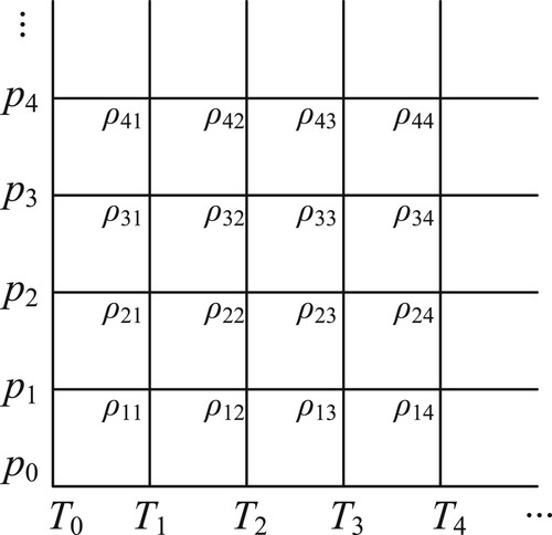
Figure A2. Schematic of TDCEE tools.

A.2. Interpolation of look-up table and interpolation errors

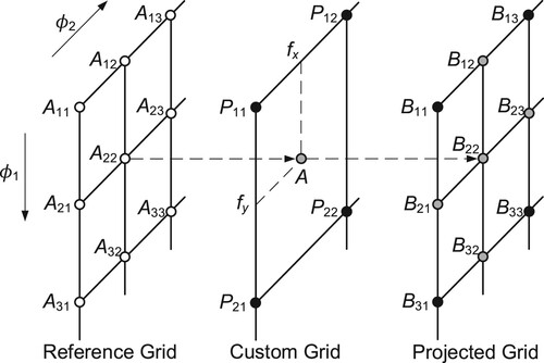
The LuT mechanism is applied once the solver calls to calculate a specific state point. With a given property table, the 2D linear interpolation method is applied to calculate a specific state point which is offset with the exact nodal points. Thus, to evaluate the interpolation errors, once the custom (coarse) and reference (fine) grids are created, a projected grid is created based on the LuT mechanism, as shown in Figure A2, marked ‘Projected Grid’. The projected grid should have the same size as the reference grid, thus direct mathematical evaluation can be applied on error estimation. The black dots denote the nodal points coincident with the custom grid, the grey dots denote the nodal points ‘projected’ from the reference grid via custom grids through the 2D linear interpolation method, which is listed as following equations: (A12) $\begin{array}{rl}{P}_{\mathrm{t}\mathrm{o}\mathrm{p}}& =(P_{a,b+1}-P_{a,b})\times f_x+P_{a,b}\end{array}$(A12) (A13) $\begin{array}{rl}{P}_{\mathrm{b}\mathrm{o}\mathrm{t}}& =(P_{a+1,b+1}-P_{a+1,b})\times f_x+P_{a+1,b}\end{array}$(A13) (A14) $\begin{array}{rl}{B}_{ij}& =(P_{\mathrm{b}\mathrm{o}\mathrm{t}}-P_{\mathrm{t}\mathrm{o}\mathrm{p}})\times f_y+P_{\mathrm{t}\mathrm{o}\mathrm{p}}\end{array}$(A14) Then a projected grid is defined as $B_{ij}$: (A15) $\begin{array}{r}{\mathbf{B}}_{ij}=\left[\begin{array}{cccc}{B}_{11}& B_{12}& \cdots & B_{1j}\\ B_{21}& B_{22}& \cdots & B_{2j}\\ ⋮& ⋮& ⋮& ⋮\\ B_{i1}& B_{i2}& \cdots & B_{ij}\end{array}\right]\end{array}$(A15)

A.3. Error evaluation for a single look-up table

The interpolation error is evaluated point by point. The error matrix for nodal points is calculated as (A16) $\begin{array}{r}{\mathbf{E}}_{ij}=\frac{{\mathbf{A}}_{ij}-{\mathbf{B}}_{ij}}{\Vert {\mathbf{A}}_{ij}\Vert }\times 100\mathrm{\%}\end{array}$(A16) ${\mathbf{E}}_{ij}$ is (A17) $\begin{array}{r}{\mathbf{E}}_{ij}=\left[\begin{array}{cccc}{E}_{11}& E_{12}& \cdots & E_{1j}\\ E_{21}& E_{22}& \cdots & E_{2j}\\ ⋮& ⋮& ⋮& ⋮\\ E_{i1}& E_{i2}& \cdots & E_{ij}\end{array}\right]\end{array}$(A17) Then the maximum error of this grid will be returned and marked as ${ϵ}_{m;i,j}$.

A.4. Automated table evaluation

To find the best resolution of the custom table grids, a series of custom grids should be created and evaluated with the reference grid. Thus, a series of discretization numbers for ${\varphi }_0$ and ${\varphi }_1$ for user-defined grids are set. For ${\varphi }_0$, the discretization number is set from a to b. Because at least two nodal points are required to form one coordinate axis of a table, that a should be greater than or equal to two. To do a meaningful combination scan, another condition, i.e. b>a, is required. Similarly, the nodal number from c to d is set for ${\mathit{\Phi }}_{\mathit{1}}$. Thus, a series of custom grids with different resolutions, from $a\times c$ to $b\times d$, are created. In order to describe the calculation method clearly, a $(b-a)\times (d-c)$ matrix is constructed as (A18) $\begin{array}{r}{\mathbf{S}}_{b-a,d-c}=\left[\begin{array}{ccccc}{\mathbf{P}}_{a,c}& {\mathbf{P}}_{a+1,c}& \cdots & {\mathbf{P}}_{b-1,c}& {\mathbf{P}}_{b,c}\\ {\mathbf{P}}_{a,c+1}& {\mathbf{P}}_{a+1,c+1}& \cdots & {\mathbf{P}}_{b-1,c+1}& {\mathbf{P}}_{b,c+1}\\ ⋮& ⋮& \ddots & ⋮& ⋮\\ {\mathbf{P}}_{a,d-1}& {\mathbf{P}}_{a+1,d-1}& \cdots & {\mathbf{P}}_{b-1,d-1}& {\mathbf{P}}_{b,d-1}\\ {\mathbf{P}}_{a,d}& {\mathbf{P}}_{a+1,d}& \cdots & {\mathbf{P}}_{b-1,d}& {\mathbf{P}}_{b,d}\end{array}\right]\end{array}$(A18) where each ${\mathbf{P}}_{mn}$ is an $m\times n$ custom grid, as shown in Figure A2. The nodal points matrix for ${\mathbf{P}}_{mn}$ is listed in Equation (A10(A10) $\begin{array}{r}{\mathbf{P}}_{mn}=\left[\begin{array}{cccc}{P}_{11}& P_{12}& \cdots & P_{1n}\\ P_{21}& P_{22}& \cdots & P_{2n}\\ ⋮& ⋮& \ddots & ⋮\\ P_{m1}& P_{m2}& \cdots & P_{mn}\end{array}\right]\end{array}$(A10) ). Then a matrix that stores all projected matrices is listed as (A19) $\begin{array}{r}{\mathbf{V}}_{b-a,d-c}=\left[\begin{array}{ccccc}{\mathbf{B}}_{a,c}& {\mathbf{B}}_{a+1,c}& \cdots & {\mathbf{B}}_{b-1,c}& {\mathbf{B}}_{b,c}\\ {\mathbf{B}}_{a,c+1}& {\mathbf{B}}_{a+1,c+1}& \cdots & {\mathbf{B}}_{b-1,c+1}& {\mathbf{B}}_{b,c+1}\\ ⋮& ⋮& \ddots & ⋮& ⋮\\ {\mathbf{B}}_{a,d-1}& {\mathbf{B}}_{a+1,d-1}& \cdots & {\mathbf{B}}_{b-1,d-1}& {\mathbf{B}}_{b,d-1}\\ {\mathbf{B}}_{a,d}& {\mathbf{B}}_{a+1,d}& \cdots & {\mathbf{B}}_{b-1,d}& {\mathbf{B}}_{b,d}\end{array}\right]\end{array}$(A19) After that, the TDCEE tool goes through every component of the matrix (A18(A18) $\begin{array}{r}{\mathbf{S}}_{b-a,d-c}=\left[\begin{array}{ccccc}{\mathbf{P}}_{a,c}& {\mathbf{P}}_{a+1,c}& \cdots & {\mathbf{P}}_{b-1,c}& {\mathbf{P}}_{b,c}\\ {\mathbf{P}}_{a,c+1}& {\mathbf{P}}_{a+1,c+1}& \cdots & {\mathbf{P}}_{b-1,c+1}& {\mathbf{P}}_{b,c+1}\\ ⋮& ⋮& \ddots & ⋮& ⋮\\ {\mathbf{P}}_{a,d-1}& {\mathbf{P}}_{a+1,d-1}& \cdots & {\mathbf{P}}_{b-1,d-1}& {\mathbf{P}}_{b,d-1}\\ {\mathbf{P}}_{a,d}& {\mathbf{P}}_{a+1,d}& \cdots & {\mathbf{P}}_{b-1,d}& {\mathbf{P}}_{b,d}\end{array}\right]\end{array}$(A18) ) to calculate the error for every component matrix. The results form the total error matrix, i.e. (A20) $\begin{array}{r}{\mathbf{W}}_{b-a,d-c}=\left[\begin{array}{ccccc}{\mathbf{E}}_{a,c}& {\mathbf{E}}_{a+1,c}& \cdots & {\mathbf{E}}_{b-1,c}& {\mathbf{E}}_{b,c}\\ {\mathbf{E}}_{a,c+1}& {\mathbf{E}}_{a+1,c+1}& \cdots & {\mathbf{E}}_{b-1,c+1}& {\mathbf{E}}_{b,c+1}\\ ⋮& ⋮& \ddots & ⋮& ⋮\\ {\mathbf{E}}_{a,d-1}& {\mathbf{E}}_{a+1,d-1}& \cdots & {\mathbf{E}}_{b-1,d-1}& {\mathbf{E}}_{b,d-1}\\ {\mathbf{E}}_{a,d}& {\mathbf{E}}_{a+1,d}& \cdots & {\mathbf{E}}_{b-1,d}& {\mathbf{E}}_{b,d}\end{array}\right]\end{array}$(A20) Continuously, the TDCEE tool will calculate the maximum error for every E${}_{xy}$ and return a new matrix that stores all the maximum errors: (A21) $\begin{array}{r}{\mathbf{E}\mathbf{M}}_{b-a,d-c}=\left[\begin{array}{cccc}{ϵ}_{m;a,c}& {ϵ}_{m;a+1,c}& \cdots & {ϵ}_{m;b,c}\\ {ϵ}_{m;a,c+1}& {ϵ}_{m;a+1,c+1}& \cdots & {ϵ}_{m;b,c+1}\\ ⋮& ⋮& \ddots & ⋮\\ {ϵ}_{m;a,d-1}& {ϵ}_{m;a+1,d-1}& \cdots & {ϵ}_{m;b,d-1}\\ {ϵ}_{m;a,d}& {ϵ}_{m;a+1,d}& \cdots & {ϵ}_{m;b,d}\end{array}\right]\end{array}$(A21) Finally, the TDCEE tool will recommend the best combination of custom grids, which has the least number of nodal points but meets the criteria.

It is convenient to plot a figure that shows the variation of ${ϵ}_m$ against the table discretization number of primitive variables. Another figure shows the distribution of errors for the recommended custom LuT. Using this figure, the user can Find which point corresponds to the maximum error ${ϵ}_m$.

A.5. Example – a look-up table for carbon dioxide

In this example, the error of a ${\mathrm{C}\mathrm{O}}_2$ density look-up table is evaluated. The pressure p and temperature T are selected as the primitive variables of the tabular value. The detail for the table to be selected is listed in Table A1.

Table C1. Details for the example.

Items	Value
Data	density
Temperature range	200–400 K
Pressure range	0.1–0.2 MPa
Resolution for reference table	$800\left(T\right)\times 800\left(p\right)$
Minimum points number for T	25
Minimum points number for p	5
Maximum points number for T	30
Maximum points number for p	10

The ranges for p and T are set to 0.1–0.2 Mpa and 200–400 K, respectively. The ranges for discretization numbers of p and T are 5–10 and 25–30. A series of user-defined grids whose total nodal points number ranges from $5\times 25=125$ to $10\times 30=300$ are created.

For the example case, the maximum errors for different $E_{ij}$ are plotted in Figure A3(a), and detailed values of ${ϵ}_m$ are listed in Table A2. It can be seen that, if the LuT has six discretization nodal points for p and six for T, the maximum error will reach 0.8971%. It is obvious that, by increasing both the p and T discretization numbers, the maximum interpolation error will drop significantly. For the $10\times 30$ table grid, the maximum error drops to 0.3744%.

Figure A3. Error graph of the TDCEE tool: (a) maximum error for all selected combinations of T and p; and (b) error value of selected nodal points.

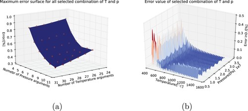
Table C2. Look-up table accuracy for the example case (%).

	$N_i$
$N_j$	25	26	27	28	29	30
5	0.8971	0.8800	0.8641	0.8502	0.8410	0.8324
6	0.7162	0.6999	0.6848	0.6706	0.6574	0.6450
7	0.5995	0.5839	0.5693	0.5556	0.5429	0.5309
8	0.5335	0.5050	0.4907	0.4774	0.4649	0.4531
9	0.5369	0.4986	0.4627	0.4292	0.4100	0.3986
10	0.5363	0.4980	0.4622	0.4287	0.3972	0.3744

As the benchmark error is set to 0.5% for the example case, then the TDCEE will compare every ${ϵ}_{m;i,j}$ to select the ones that satisfy the benchmark condition. Then, all the corresponding $P_{m,n}$ that pass the benchmark condition are selected. Finally, the minimal combination of $m\times n$ is selected.

Regarding the example case, it can be seen from Figure A3(a) that there are 14 ${\mathbf{P}}_{mn}$ whose ${ϵ}_m$ are smaller than 0.5%. It is obvious that ${\mathbf{P}}_{8,27}$ has fewer nodal points ($8\times 27=216$), thus the TDCCE tool recommends using ${\mathbf{P}}_{8,27}$ as the custom grid. The error matrix for ${\mathbf{P}}_{8,27}$, which is denoted as ${\mathbf{E}}_{8,27}$, is plotted as a surface map as shown in Figure A3(b). It can be seen from Figure A3(b) that ${ϵ}_m$ happens near the lower temperature region, and pressure has less influence on error compared with temperature. The work can be summarized and explained briefly by stating that, for a simulation case the pressure of which is within the range 90–200 kPa while the temperature is within the range 200–400 K, the density property can be interpolated through an $8\times 27$ nodal points table. The tabular data has an accuracy such that the maximum error is lower than 0.5%.

A test case with the OpenFOAM real gas solver RGDFoam was carried out to show the reduction in required computational resources. The test case had about 69,500 cells, running on an Intel${}^{\circledR }$ Core${}^{\mathrm{t}\mathrm{m}}$ i7-4770 CPU 3.40 GHz chip with 16.0 GB of memory. Three simulations were carried out: $200\times 200$ LuT, $30\times 30$ and PR EoS. The average serial calculation times for one iterative step were 0.31, 0.19 and 0.65 s, respectively. Thus the reduction in required computational resources was significant.

References

- Abdol-Hamid K. S., Elmiligui A., & Hunter C. A. (2006). Numerical investigation of flow in an over-expanded nozzle with porous surfaces. Journal of Aircraft, 43(4), 1217–1225. https://doi.org/10.2514/1.18835
- Arts T., Lambertderouvroit M., & Rutherford A. (1990). Aero-thermal investigation of a highly loaded transonic linear turbine guide vane cascade. A test case for inviscid and viscous flow computations (NASA STI/Recon Tech. Rep. No. 91). https://ui.adsabs.harvard.edu/abs/1990STIN...9123437A
- Batten P., Leschziner M., & Goldberg U. (1997). Average-state Jacobians and implicit methods for compressible viscous and turbulent flows. Journal of Computational Physics, 137(1), 38–78. https://doi.org/10.1006/jcph.1997.5793
- Beaudoin M., & Jasak H. (2008). Development of a generalized grid interface for turbomachinery simulations with OpenFOAM. In Proceedings of the open source CFD international conference (Vol. 2), ICON plc. https://www.researchgate.net/publication/254000473_Development_of_a_Generalized_Grid_Interface_for_Turbomachinery_simulations_with_OpenFOAM
- Borm O., Jemcov A., & Kau H. P. (2011). Density based Navier–Stokes solver for transonic flows. In Proceedings of the 6th OpenFOAM Workshop. PennState University, University Park, PA.
- Borm O., & Kau H. P. (2012). Unsteady aerodynamics of a centrifugal compressor stage–validation of two different CFD solvers Unsteady aerodynamics of a centrifugal compressor stage – validation of two different CFD solvers. In Proceedings of ASME turbo expo 2012: Turbine technical conference and exposition. American Society of Mechanical Engineers. https://doi.org/10.1115/GT2012-69636
- Chen H., Goswami D. Y., & Stefanakos E. K. (2010). A review of thermodynamic cycles and working fluids for the conversion of low-grade heat. Renewable and Sustainable Energy Reviews, 14(9), 3059–3067. https://doi.org/10.1016/j.rser.2010.07.006
- Colonna P., Nannan N., & Guardone A. (2008). Multiparameter equations of state for siloxanes: [(CH 3) 3-Si-O 1/2] 2-[O-Si-(CH 3) 2] i=1,…,3 and [O-Si-(CH 3) 2] 6. Fluid Phase Equilibria, 263(2), 115–130. https://doi.org/10.1016/j.fluid.2007.10.001
- Colonna P., Nannan N., Guardone A., & van der Stelt T. (2009). On the computation of the fundamental derivative of gas dynamics using equations of state. Fluid Phase Equilibria, 286(1), 43–54. https://doi.org/10.1016/j.fluid.2009.07.021
- Colonna P., & Rebay S. (2004). Numerical simulation of dense gas flows on unstructured grids with an implicit high resolution upwind Euler solver. International Journal for Numerical Methods in Fluids, 46(7), 735–765. https://doi.org/10.1002/(ISSN)1097-0363
- Colonna P., Rebay S., Harinck J., & Guardone A. (2006). Real-gas effects in ORC turbine flow simulations: Influence of thermodynamic models on flow fields and performance parameters. In Proceedings of the European conference on computational fluid dynamics (ECCOMAS CFD 2006). https://www.researchgate.net/publication/228374344_Real-gas_effects_in_ORC_turbine_flow_simulations_Influence_of_thermodynamic_models_on_flow_fields_and_performance_parameters
- Cramer M. (1991). Nonclassical dynamics of classical gases. In Nonlinear waves in real fluids (pp. 91–145). Springer.
- Cramer M., & Crickenberger A. (1992). Prandtl–Meyer function for dense gases. AIAA Journal, 30(2), 561–564. https://doi.org/10.2514/3.10956
- Dostal V., Driscoll M. J., & Hejzlar P. (2004). A supercritical carbon dioxide cycle for next generation nuclear reactors [Unpublished doctoral dissertation]. Department of Nuclear Engineering, Massachusetts Institute of Technology.
- Drikakis D., & Tsangaris S. (1993). On the solution of the compressible Navier–Stokes equations using improved flux vector splitting methods. Applied Mathematical Modelling, 17(6), 282–297. https://doi.org/10.1016/0307-904X(93)90054-K
- Durá Galiana F. J., Wheeler A. P., & Ong J. (2016). A study of trailing-edge losses in organic Rankine cycle turbines. Journal of Turbomachinery, 138(12), Article ID 121003. https://doi.org/10.1115/1.4033473
- Economon T. D., Palacios F., Copeland S. R., Lukaczyk T. W., & Alonso J. J. (2015). SU2: An open-source suite for multiphysics simulation and design. AIAA Journal, 54(3), 828–846. https://doi.org/10.2514/1.J053813
- Einfeldt B. (1988). On Godunov-type methods for gas dynamics. SIAM Journal on Numerical Analysis, 25(2), 294–318. https://doi.org/10.1137/0725021
- Ghalandari M., Mirzadeh Koohshahi E., Mohamadian F., Shamshirband S., & K. W. Chau (2019). Numerical simulation of nanofluid flow inside a root canal. Engineering Applications of Computational Fluid Mechanics, 13(1), 254–264. https://doi.org/10.1080/19942060.2019.1578696
- Gori G. (2019). Non-ideal compressible-fluid dynamics: Developing a combined perspective on modeling, numerics and experiments [PhD Thesis, Politecnico di Milano].
- Gori G., Zocca M., Cammi G., Spinelli A., & Guardone A. (2017). Experimental assessment of the open-source SU2 CFD suite for ORC applications. Energy Procedia, 129, 256–263. https://doi.org/10.1016/j.egypro.2017.09.151
- He Z., Zhou K., Liu S., Xiong W., & Li B. (2013). Numerical modeling of the fluid flow in continuous casting tundish with different control devices. Abstract and Applied Analysis, 2013, Article ID 984894, 8pp. https://doi.org/10.1155/2013/984894
- Head A. J., De Servi C., Casati E., Pini M., & Colonna P. (2016). Preliminary design of the ORCHID: A facility for studying non-ideal compressible fluid dynamics and testing ORC expanders. In Proceedings of ASME turbo expo 2016. American Society of Mechanical Engineers. https://doi.org/10.1115/GT2016-56103
- Head A. J., Iyer S., De Servi C., & Pini M. (2017). Towards the validation of a CFD solver for non-ideal compressible flows. Energy Procedia, 129, 240–247. https://doi.org/10.1016/j.egypro.2017.09.149
- Hunter C. A. (2004). Experimental investigation of separated nozzle flows. Journal of Propulsion and Power, 20(3), 527–532. https://doi.org/10.2514/1.4612
- Jasak H. (2013). openFOAM extensions, foam-extension 3.0 release note [Computer software]. OpenFOAM. Retrieved December 18, 2013, from https://sourceforge.net/projects/openfoam-extend/files/foam-extend-3.0/
- Jasak H., & Beaudoin M. (2011). OpenFOAM turbo tools: From general purpose CFD to turbomachinery simulations. In ASME-JSME-KSME joint fluids engineering conference (AJK2011-FED) (pp. 1801–1812). American Society of Mechanical Engineers. https://doi.org/10.1115/AJK2011-05015
- Jassim E., Abdi M. A., & Muzychka Y. (2008). Computational fluid dynamics study for flow of natural gas through high-pressure supersonic nozzles: Part 1. Real gas effects and shockwave. Petroleum Science and Technology, 26(15), 1757–1772. https://doi.org/10.1080/10916460701287847
- Kalra C., Sevincer E., Brun K., Hofer D., & Moore J. (2014). Development of high efficiency hot gas turbo-expander for optimized CSP supercritical CO 2 power block operation. In Proceedings of the 4th international symposium – supercritical CO 2 power cycles (Vol. 2, pp. 9–10). KC ORC. http://sco2symposium.com/papers2014/turbomachinery/74-Kalra.pdf
- Lemmon E. W., Huber M., & McLinder M. (2013). NIST reference database 23: Reference fluid thermodynamic and transport properties – REFPROP (version 9.1). National Institute of Standards and Technology, Standard Reference Data Program. https://www.semanticscholar.org/paper/NIST-Standard-Reference-Database-23%3A-Reference-and-Lemmon-Huber/7e649b09a1248ffff712def40d499c03776bf7d3
- Lemmon E. W., Jacobsen R. T., Penoncello S. G., & Friend D. G. (2000). Thermodynamic properties of air and mixtures of nitrogen, argon, and oxygen from 60 to 2000 K at pressures to 2000 MPa. Journal of Physical and Chemical Reference Data, 29(3), 331–385. https://doi.org/10.1063/1.1285884
- Loewenberg M. F., Laurien E., Class A., & Schulenberg T. (2008). Supercritical water heat transfer in vertical tubes: A look-up table. Progress in Nuclear Energy, 50(2), 532–538. https://doi.org/10.1016/j.pnucene.2007.11.037
- Luo H., Baum J. D., & Löhner R. (2004). On the computation of multi-material flows using ALE formulation. Journal of Computational Physics, 194(1), 304–328. https://doi.org/10.1016/j.jcp.2003.09.026
- Maraver D., Royo J., Lemort V., & Quoilin S. (2014). Systematic optimization of subcritical and transcritical organic Rankine cycles (ORCs) constrained by technical parameters in multiple applications. Applied Energy, 117(March), 11–29. https://doi.org/10.1016/j.apenergy.2013.11.076
- Menter F., & Esch T. (2001). Elements of industrial heat transfer predictions. In Proceedings of the16th Brazilian congress of mechanical engineering (COBEM) (Vol. 20). Amsterdam, Netherlands: IOS press.
- Palacios F., Colonno M. R., Aranake A. C., Campos A., Copeland S. R., T. D. Economon, Lonkar A. K., Lukaczyk T. W., Taylor T. W. R., & Alonso J. J. (2013). Stanford University Unstructured (SU2): An open-source integrated computational environment for multi-physics simulation and design. In Proceedings of the 51st AIAA aerospace sciences meeting including the new horizons forum and aerospace exposition, AIAA paper 2013-0287 (p. 287). American Institute of Aeronautics and Astronautics. https://doi.org/10.2514/6.2013-287
- Pini M., Spinelli A., Persico G., & Rebay S. (2015). Consistent look-up table interpolation method for real-gas flow simulations. Computers & Fluids, 107, 178–188. https://doi.org/10.1016/j.compfluid.2014.11.001
- Qi J. (2017). RGDFoam [Computer software]. GitHub. https://github.com/cyjanry/RGDFoam_v1/
- Qi J., Reddell T., Qin K., Hooman K., & Jahn I. H. (2017). Supercritical CO 2 radial turbine design performance as a function of turbine size parameters. Journal of Turbomachinery, 139(8), Article 081008. https://doi.org/10.1115/1.4035920
- Qiu J. (2021). Numerical simulations of non-ideal supersonic nozzle expansions.
- Reis A. J. F. (2013). Validation of NASA Rotor 67 with OpenFOAM's transonic density-based solver [Unpublished doctoral dissertation]. Faculdade de Ciências e Tecnologia, Universidade Nova Di Lisboa.
- Roe P. L. (1981). Approximate Riemann solvers, parameter vectors, and difference schemes. Journal of Computational Physics, 43(2), 357–372. https://doi.org/10.1016/0021-9991(81)90128-5
- Salih S. Q., Aldlemy M. S., Rasani M. R., Ariffin A., Ya T. M. Y. S. T., Al-Ansari N., Yaseen Z. M., & Chau K. W. (2019). Thin and sharp edges bodies-fluid interaction simulation using cut-cell immersed boundary method. Engineering Applications of Computational Fluid Mechanics, 13(1), 860–877. https://doi.org/10.1080/19942060.2019.1652209
- Smith M. J., Potsdam M., Wong T. C., Baeder J. D., & Phanse S. (2006). Evaluation of computational fluid dynamics to determine two-dimensional airfoil characteristics for Rotorcraft applications. Journal of the American Helicopter Society, 51(1), 70–79. https://doi.org/10.4050/1.3092879
- Span R., & Wagner W. (1996). A new equation of state for carbon dioxide covering the fluid region from the triple-point temperature to 1100 K at pressures up to 800 MPa. Journal of Physical and Chemical Reference Data, 25(6), 1509–1596. https://doi.org/10.1063/1.555991
- The OpenFOAM Foundation (2016). OpenFOAM v5 user guide [Computer software manual]. https://cfd.direct/openfoam/user-guide
- Thompson P. A. (1971). A fundamental derivative in gasdynamics. The Physics of Fluids, 14(9), 1843–1849. https://doi.org/10.1063/1.1693693
- Thompson P. A., & Lambrakis K. (1973). Negative shock waves. Journal of Fluid Mechanics, 60(1), 187–208. https://doi.org/10.1017/S002211207300011X
- Van Leer B. (1977). Towards the ultimate conservative difference scheme. IV. A new approach to numerical convection. Journal of Computational Physics, 23(3), 276–299.
- Van Leer B. (1982). Flux-vector splitting for the Euler equations. In Upwind and high-resolution schemes (pp. 80–89). Berlin: Springer.
- Vitale S., Albring T. A., Pini M., Gauger N. R., & Colonna P. (2017). Fully turbulent discrete adjoint solver for non-ideal compressible flow applications. Journal of the Global Power and Propulsion Society, 1, 252–270. https://doi.org/10.22261/JGPPS
- Vitale S., Gori G., Pini M., Guardone A., Economon T. D., Palacios F., J. J. Alonso, & Colonna P. (2015). Extension of the SU2 open source CFD code to the simulation of turbulent flows of fluids modelled with complex thermophysical laws. In Proceedings of the 22nd AIAA computational fluid dynamics conference (pp. 1–22). American Institute of Aeronautics and Astronautics.
- Wang J., Huang Y., Zang J., & Liu G. (2015). Recent research progress on supercritical carbon dioxide power cycle in China. In Proceedings of ASME turbo expo 2015: Turbine technical conference and exposition. American Society of Mechanical Engineers. https://doi.org/10.1115/GT2015-43938.
- Weller H. G., Tabor G., Jasak H., & Fureby C. (1998). A tensorial approach to computational continuum mechanics using object-oriented techniques. Computers in Physics, 12(6), 620–631. https://doi.org/10.1063/1.168744
- Wright S. A., Radel R. F., Vernon M. E., Rochau G. E., & Pickard P. S. (2010). Operation and analysis of a supercritical CO 2 Brayton cycle (Tech. Rep. No. SAND2010-0171). Sandia.
- Xu J., Liu C., Sun E., Xie J., Li M., Yang Y., & Liu J. (2019). Perspective of S-CO 2 power cycles. Energy, 186, Article 115831.
- Zhan Y., & Sapatnekar S. S. (2005). Fast computation of the temperature distribution in VLSI chips using the discrete cosine transform and table look-up. In Proceedings of the 2005 Asia and South Pacific design automation conference (pp. 87–92). New York, NY: Association for Computing Machinery.