Field measurements and CFD simulations of wind characteristics at the Yellow River bridge site in a converging-channel terrain

Abstract

This paper is aimed at investigating the airflow over unusual converging-channel terrain that includes a deep valley on the up-river side and a flat plain on the down-river side. A computational fluid dynamics (CFD) simulation with standard k–ε model was applied to study the variation of wind structure from the important approach wind directions. A long-period of field measurements provided supplementary data from a Sodar system and also 2D ultrasonic anemometers. Broad agreement was found between the observations and the CFD simulations. The results show that a wind speed-up was generated in the valley and its exit, whose magnitude was sensitive to the approaching wind direction, and that terrain-induced effects on wind direction are significant within the height range up to 200 m. It is also found that the wind speeds and directions along the entire bridge structure, including the spanwise deck and the bridge towers, is non-homogeneous due to the effects of the complex terrain. Moreover, through comparing the predicted wind speed at this bridge site, it was found that the Chinese national code recommends a lower speed than CFD simulations for the two worst approach directions which are normal to the bridge axis.

KEYWORDS:

• Wind characteristics
• complex terrain
• bridge site
• CFD simulations
• field measurement

1. Introduction

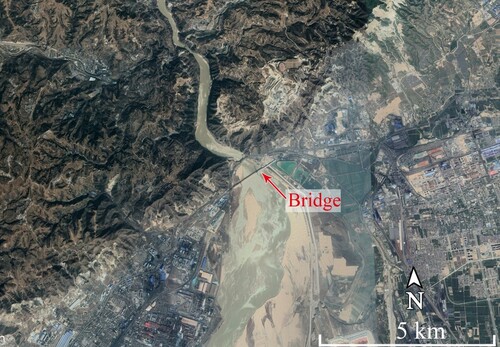
Wind loading of structures has been researched extensively in many countries over many years. Wind actions are critical, particularly for flexible bridges; therefore, there have been extensive wind studies on topics including wind field characteristics at bridge sites, wind resistance, and wind response of bridge structures. However, wind characteristics vary significantly depending on the type of terrain, so researchers should consider each representative terrain. In this paper, we aimed to investigate wind characteristics at an unusual and very interesting bridge site near a deep valley in a mountain range where the river enters a plain (Figure 1).

Figure 1. Bridge location and surrounding terrain.

Wind tunnel tests, field measurements and CFD simulations are commonly used in wind characteristics research. There are many published papers proving the feasibility and precision of field measurements. Little (1969) demonstrates that the acoustics echo-sounding method (Sodar) is entirely feasible for measuring the vertical profile of wind speed and direction for the lower atmosphere using Doppler radar and three-dimensional turbulence through both monostatic and biostatic radars. Vogt and Thomas (1995) show that Sodar can obtain reliable wind velocity and turbulence data by comparing Sodar and cup-anemometer data. These methods have been utilized in atmospheric boundary layer (ABL) research for many years. Song et al. (2020) studied a bridge site in a mountainous area using a Sodar system and analysed the difference with wind tunnel tests. They found that there was significant influence on wind direction and turbulence along the bridge span caused by valley and the local terrain, and the wind characteristics along the bridge deck were non-homogenous. CFD simulation is highly praised by researchers because of its economy and efficiency. It is similarly important for CFD to accurately simulate. Ghalandari et al. (2019) made a comparison among presented differential method formulations. For airflow over complex terrain, first of all, setting up a horizontally homogeneous ABL in the entire computational domain is an essential requirement for authentic wind speed prediction. Richards and Hoxey (1993) propose appropriate boundary profiles associated with the k–ε turbulence model to simulate homogeneous flow. Richards and Norris (2015) also provide applicative inlet profiles for a pressure-driven ABL for RANS simulations with k–ε, k–ω, and SST turbulence models. Blocken et al. (2007) emphasize that simulating a horizontally homogeneous ABL requires both exact boundary conditions as well as high-quality computational grids, and presented the key to the wall function problem, by deriving the relationship between the local aerodynamic roughness and sand-grain roughness in many CFD codes, and declared that the height of the wall-adjacent cells should be larger than twice the sand-grain roughness height. Salih et al. (2019) provided a helpful meshing method to simulate airflow in the boundary layer over a complex surface. Over the past several decades, many studies have focused on predicting airflow over complex terrain, and the results could be verified by field measurements and wind tunnel test. An example of a large co-ordinated research project focused on wind characteristics over hills is the Askervein Hill project (1985, 1987, 1987, 1996) which has been studied by many researchers. When Raithby et al. (1987) revised the standard k–ε model and applied 3D RANS simulation to investigate the airflow over Askervein, the results agreed with the field measurements in the mean airflow variables, speed-up, and direction. Moreover, Pirooz and Flay (2018) investigated the speed-up over a simplified hill by undertaking CFD simulations and wind tunnel tests, and consistent results were found between them. Pirooz et al. (2019) carried out RANS and hybrid RANS/LES simulations to model the airflow over hills and found that consistent results were obtained in the wake region for mean speedups. Flay et al. (2019), studied wind flow over the Belmont Hill in New Zealand by observations and modeling using CFD codes and wind tunnel tests and found good agreement among them in some cases. Blocken et al. (2015) used a 3D steady RANS model and a realizable k–ε model to simulate air flow over Ria de Ferrol on the NW coast of Spain which is a complex bay including a narrow channel surrounded by valleys. There was a good agreement between simulation results and field measurements, indicating that the 3D steady RANS with the realizable k–ε model could accurately simulate this natural complex terrain.

There are method and numerous results of studies on wind characteristics over complex terrain in the ABL. However, few researchers have studied converging-channel terrain, like the unusual Yellow River bridge site (35°39′21′′ N, 110°36′12′′ E), which is the subject of this paper. Therefore, in the present paper the spatial airflow over this dramatically changing terrain is investigated by using field measurements from Doppler Sodar and two ultrasonic anemometers, and a 3D steady RANS simulation with the standard k–ε model.

The outline of the paper is as follows: Section 2 introduces basic information about the terrain and details of the field measurement arrangements and the CFD simulation. Section 3 analyses the field measurement results, mainly focusing on the mean wind speed and direction, and the turbulence characteristics. Section 4 validates the CFD simulation through comparison with the field measurements, and discusses the spatially varying distribution of wind characteristics. In Section 5 the results of both the CFD study and the field observations are compared to predicted values from the Chinese national wind code.

2. Methodology

2.1. Bridge location and surrounding terrain

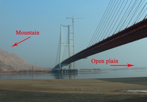
A cable-stayed bridge spanning the Yellow River has been constructed as shown in Figure 1. It can be seen that the topography is dramatic where the Yellow River enters the plain from the mountainous valley. The Yellow River creates a horn-shaped fluvial bank and then widens sharply into the river channel. The bridge is located in the valley-widening section. Figure 2 shows the scene of the bridge site photographed by the authors after bridge closure. It shows that there is mountainous area on the one side (NW side) of the bridge and an open plain on the other side (SE side). It can also be seen in Figure 2 that the bridge tower is built in an H-shape and each is more than 160 m high. The main span is 1055 m with a π-shape girder structure combining twin steel I-beams and a concrete deck. This type of bridge deck is becoming increasingly popular because the mechanical and economic advantages of both steel and concrete can be reasonably employed compared with other shapes. However, a disadvantage of this bluff-body girder shape is its fairly low structural frequency and it is therefore susceptible to dynamic excitation by the wind load.

Figure 2. The scene viewed from northwest of the bridge.

2.2. Field monitoring arrangement

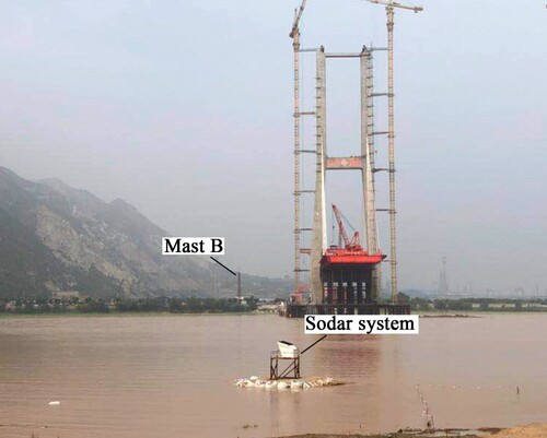
The observation station was equipped with instruments after bridge construction was started in 2017. The on-site station was equipped with a Model VT-1 Phased-Array Doppler Sodar System and two Gill Wind Sonics. The Sodar System, a remote sensor for wind vertical profile detection, was placed in the southwest basin of the river, which is located northwest of the bridge. The Gill Wind Sonic is a 2D ultrasonic anemometer for detecting horizontal wind speed and direction. There are anemometers located at the top of both masts which are 60 m high and marked as Masts A and B in Figure 3. Figure 4 is a site photograph taken in July 2018 and displays an overview of the wind monitoring arrangement with locations.

Figure 3. Bridge site and key locations.

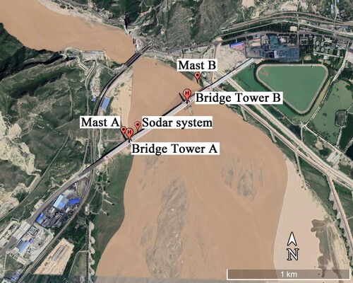
Figure 4. Locations of observation instruments.

2.3. CFD simulation

2.3.1. Geometry and mesh

The CFD simulation was carried out inside the red circle shown in Figure 5, a circular area with a 10 km diameter, trimmed slightly in one region so that the boundary was located in a pass between two mountain ranges. The center of the selected area is at the middle of the bridge span.

Figure 5. CFD modeled area, showing terrain roughness and approaching airflow directions.

The terrain geometry was generated using high-resolution GIS data. A larger circle was specified to envelope the modeled terrain region in order to loft a slope from the height of the terrain at the edge of the modeled region down to zero height at the outer circle to obtain a smooth flow transition at the edge. To develop a horizontally homogeneous ABL, the distance from the computational inlet to the modeled terrain block should be in the range of 5–10 km. The maximum valley depth in the mountains to the northwest of the bridge is 420 m, and the height of the ABL was estimated to be 1500 m assuming U(10) = 10 m/s and z₀ = 0.3 m. Therefore, considering the experience and advice of other researchers (Blocken et al., 2015; Franke, 2007), the computational domain was sized at 35 km long × 25 km wide × 2.0 km high and extended above the top of the ABL.

A triangular mesh was used for the computational grid at the bottom of the domain with mesh refinement on the terrain surface, as shown in Figure 6. In the terrain modeled area, prismatic cells were generated by inflation within the first 500 m. These meshes were body-fitted and stay parallel with a complex terrain surface. Many researchers have demonstrated that a prismatic and hexahedral grid can be of controllable resolution and quality. Blocken et al. (2007) proposed that the height of the wall-adjacent cells should be twice the size of k_s of the local terrain and defined the connection between the aerodynamic roughness length z₀ and the wall function parameter k_s in CFX as in Equation (1(1) $k_s=29.6z_0$(1) ). (1) $k_s=29.6z_0$(1)

Figure 6. Surface mesh of the modeled terrain.

To determine the value of z₀, Blocken et al. (2015) use two types of aerodynamic roughness to simulate wind flow for Ria de Ferrol. One type is used to represent the roughness of the study area surface while the other is used to set up the inlet profile based on the roughness of the surrounding topography in the computational domain.

In the present study area, the local z₀ is estimated to be 0.025 m for the vegetated hills and buildings in the urban areas, corresponding to regions A, B, C and D inside the red circle in Figure 5, and is 0.01 m for the Yellow River and sandy shore (shown as region E). Moreover, there is a large difference between northwest and southeast upstream surrounding topography outside the red circle, and therefore, as Figure 5 shows, it was assumed that z₀ = 0.25 m for the northwest quadrant and z₀ = 0.05 m for the southeast quadrant.

Additionally, for an accurate ABL flow simulation it is essential to generate a high-resolution mesh near the terrain surface to allow for the two values of the first-layer thicknesses for the terrain and the extended areas.

2.3.2. Boundary and solver settings

In this study, the pressure-driven approach was employed using the CFX package, and a k_s-type wall function was used for generating the ABL. Richards and Norris (2015) derived velocity and turbulence profiles for this case, which were applied successfully by Pirooz and Flay (2018) to compute speed-up over simple hills and shows good agreement with their wind tunnel tests. Equations (2)-(4) are recommended for the standard k–ε turbulence models and were used to set up the inlet boundary conditions in the present study. (2) $\begin{array}{rl}U(z)& =(u_{\tau }/\kappa )\times (\ln (z/z_0)+C_{U1}(z/H)+C_{U2}{(z/H)}^2\\ & +C_{U3}{(z/H)}^3+C_{U4}{(z/H)}^4)\end{array}$(2) (3) $\begin{array}{rl}k(z)& =u_{\tau }^2[C_{k1}+C_{k2}{(1-z/H)}^2+C_{k3}{(1-z/H)}^4\\ & +C_{k4}{(1-z/H)}^6]\end{array}$(3) (4) $\begin{array}{rl}\epsilon (z)& =C_{\mu }k(z{)}^2/\kappa u_{\tau }z\times [1+(1+C_{u1})(z/H)\\ & +(1+C_{u1}+2C_{u2}){(z/H)}^2\\ & +(1+C_{u1}+2C_{u2}+3C_{u3}){(z/H)}^3]\end{array}$(4) where the von Karman constant κ is 0.4 and C_μ is 0.09. z₀ is the aerodynamic roughness length of the terrain. H is the computational domain height and is specified in Section 2.3. The friction velocity, u_τ, can be calculated by assuming a reference velocity. The polynomial coefficients, also provided by Richards and Norris (2015), are given in Table 1.

Table 1. Polynomial coefficients (Blocken et al., 2015).

Ck1	Ck2	Ck3	Ck4
0.921	3.533	−1.926	0.805
CU1	CU2	CU3	CU4
0.528	0.385	−1.09	0.243

The bottom of the computational domain is modeled as a no-slip wall with the appropriate values of k_s. The top and lateral boundaries were set as symmetry boundary types, and the outlet boundary type was set to zero-pressure.

2.3.3. Grid-sensitivity analysis

The grid-sensitivity analysis procedure recommended by Celik (2008) is aimed to investigate grid independence by calculating parameters including the grid-refinement factor r, extrapolated values φ_ext, relative errors e_a, extrapolated relative errors e_ext and the grid-convergence index GCI. Firstly, a grid-sensitivity analysis must be carried out in an empty domain to check the horizontal homogeneity of the ABL in the entire computational domain. Three precision levels of grids were generated, with first layer heights of 18, 24, and 20 m at growth rates of 1.15, 1.2, and 1.25, respectively. The analysis focused on the mean wind speed in the inlet, middle and outlet of the computational domain and resulted in the adoption of the finest grid for this investigation. The ABL horizontal homogeneity investigation results are shown in Figure 7. The sharp change in the TKE profile at low levels is caused by discretization errors in the near-wall region (Richards & Norris, 2011) and a recognized feature is the existence of a peak in the second-layer cells in the k–ε model (Hargreaves & Wright, 2007). It can be seen that the flow domain has excellent horizontal homogeneity.

Figure 7. ABL horizontal homogeneity investigation results. (a) Velocity profiles. (b) TKE profiles. (c) TED profiles.

A grid-sensitivity analysis was employed in the study domain, using three grids with fine, medium, and coarse precision levels. The first-layer thickness is defined as 3, 4, and 5 m with growth rates of 1.15, 1.2, and 1.25, respectively. The results are given in Table 2 at the inlet, central region and at the outlet. The fine mesh was used in the following analysis with 3,045,702 prismatic elements.

Table 2. Results of the discretization error investigation for the fine, medium and coarse grids.

Total number of cells N1, N2, N3	3,045,702 995,139 454,024
Grid refinement factor r21, r32	1.45, 1.30
Solution	φ = Inlet velocity at x/H = 1, y = 0, z = 500 m	φ = Central velocity at x/H = 7, y = 0, z = 500 m	φ = Outlet velocity at x/H = 15, y = 0, z = 500 m
φ1, φ2, φ3 (m s^−1)	21.48, 21.50, 21.06	19.62, 19.62, 19.64	21.23, 21.15, 21.06
φext^21 (m s^−1)	21.48	19.62	21.58
ea^21 (%), eext^21 (%)	0.06, 0.01	0.002, 0.00	0.39, 1.60
GCIfine^21 (%)	0.01	0.00	2.03

3. Discussion of field measurement data

3.1. Measured data recording and screening

The Sodar System outputs the mean wind data, including horizontal wind speed and wind direction, wind speed components, and sample reliability, for each 10-minute period. The equipment was set up and orientated with respect to true north, the wind direction is measured in degrees clockwise from true north. The wind speed is represented in three orthogonal components: north-south, east-west, and vertical. The acceptance criteria for the recorded data used in this research requires reliability values of 9, meaning that random signal noise in the analysed measurements was negligible. Eighteen wind vector data collection points were set up in a vertical line from 30 to 200 m at 10 m intervals. The bridge deck is around at an observed height of 40 m. The Sodar System started recording in November 2017 and finished recording in July 2018 due to the seasonal summer flood. The operation of the system was suspended for a month during this period due to power problems caused by a mechanical digger. Consequently, 216 days of Sodar System data files were available and employed in the present paper. The mast measurement system was running during the same period as Sodar system at a sampling frequency of 4 Hz. All reliable records were used in the database.

3.2. Mean wind characteristics

The wind direction and speed are discussed in this section and there is no discussion of the inclination angles. This is because the field equipment was located above the riverbank plane, the measured inclination angles are almost zero.

The relationship between wind direction and speed can be shown by the increase in wind speed. Figure 8 provides the Sodar system results for heights of 40, 100, 150, and 200 m. Clearly the prevailing wind direction is very consistent in a 300–330° range over all heights, corresponding to the northwest wind. This means that wind always blows out of the valley onto the plains. And the wind speed covers all the ranges. Additionally, there is a second peak in the opposite direction at 150–160° and wind speeds are mostly lower than 5 m/s. For this range of directions, the wind is blowing into the valley. It can be deduced that the airflow is accelerated when flowing through the valley.

Figure 8. Wind speed roses at four heights. (a) z = 40 m. (b) z = 100 m. (c) z = 150 m. (d) z = 200 m.

In Figure 8(a), the wind direction at a height of 40 m is shifted slightly to the west and is nearly parallel with the exit section of the valley. For the 100 m height in Figure 8(b), the shape of the roses are the most narrow and reach the highest frequencies in each wind range, indicating very strong directionality at this height. The roses get shorter and wider at heights of 150 and 200 m, in Figure 8(c,d), there are also small peaks in the north, indicating a wider range of wind directions. The changes of wind direction with altitude show the terrain-inducing effect is stronger near the ground and gets weaker above a height of 150 m.

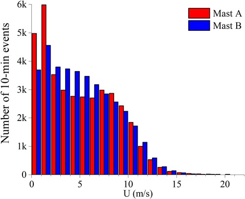
For the Mast A and B measurements, 10 min mean velocities were calculated using MATLAB R2019. Statistical analysis was employed to compare the probability densities of the velocity distributions between each mast recording. The histogram in Figure 9 shows that the distributions at higher velocities (>8 m s⁻¹) are almost identical, while for lower speeds Mast A had a much higher proportion of very low speeds compared with Mast B. This difference is because Mast B faces into the river valley, but Mast A is somewhat sheltered by hilly terrain for the prevailing wind direction of 320° out of the valley as shown in Figure 5.

Figure 9. Histogram of 10 min mean velocity.

3.3. Turbulence characteristics

Turbulent wind significantly affects aero-elastic stability phenomena, especially for shapes like this bridge deck with its bluff body profile. In this section, the turbulence intensity and spectral density measurements from the mast measurements are discussed. The along-wind turbulence intensity is calculated using Equation (5(5) $I_u={\sigma }_u/U$(5) ). (5) $I_u={\sigma }_u/U$(5) where σ_u is the standard deviation of the wind speed fluctuations in the along-wind direction and U is the 10-min mean wind velocity.

A windy day, 29 December 2017, was selected from the Sodar system database for further analysis. The mean wind direction for this period was 315° so the wind was directed out of the valley normal to the bridge deck towards the plain. The relationship between turbulence intensity and mean velocity for this windy day is plotted in Figure 10 and shows a reasonably linear decreasing trend. The turbulence intensity is much higher at low wind speeds, as observed by others, due to the very unsteady nature of low speed wind flow when there is a contribution of thermal effects to the turbulence.

Figure 10. Turbulence intensity versus mean velocity for 29 December 2017 for a height of 40 m and a wind direction of 315°.

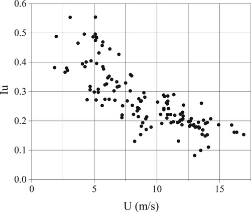
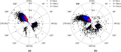
Figure 11 shows a polar plot of the turbulence intensity values from Masts A and B for wind speed thresholds of 5, 10 and 15 m s⁻¹. As expected, the turbulence intensities for the lowest wind speed threshold vary considerably and can be very large due to the very unsteady nature of low speed winds, which is in agreement with the Sodar system results. Most of the points are clustered in the direction of the prevailing NW and SE winds, but there is also a contribution from the SW for the lowest speed band. For the higher threshold speeds of 10 and 15 ms⁻¹ (blue and red respectively) most data are concentrated in the sector 300–330°, as for the mean wind speed data in Figure 8. In addition, the turbulence intensity for these higher speeds reduces and most of the data lie in the range of 0.1–0.3. This is because for these higher speeds the boundary layer is neutrally stable and thermal effects will not be very significant.

Figure 11. Turbulence intensity roses for two wind sonics on Masts A (left) and B (right).

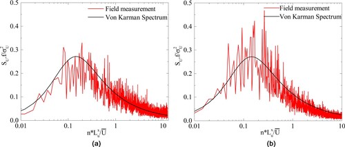
Along-wind turbulence spectra are estimated through representative recordings measured in a windy period during 6:00–9:00 am on the same windy day 29 December 2017 with a mean velocity of 11.4 m s⁻¹ for mast A and 11.9 m s⁻¹ for mast B. Furthermore, power spectral densities were plotted to describe the turbulence in the frequency domain, and are fitted by the von Karman spectrum in Figure 12. The integral length scales used to fit the measured spectra to the von Karman spectra were calculated by integrating the autocorrelation function and then by multiplying by the mean wind speed, thus invoking Taylor’s hypothesis. The values obtained from this method for the Mast A and B data are 71 and 60 m respectively. It can be seen that the measured spectra from both masts are well fitted by the von Karman spectrum. In particular the slope of the high frequency part of the curve in the inertial subrange region agrees with the von Karman spectrum. Considering the mast tower location with respect to upstream obstructions, there are some minor discrepancies between two spectra. The spectral density of mast A is slightly flatter than mast B.

Figure 12. Wind speed spectral density estimates for 6:00–9:00 am on 29 December 2017 for a wind direction of 315° out of the valley.

For wind flow over water at a height of 40 m, ESDU85020 (1985) can be used to estimate the integral length scale, resulting in a value of about 200 m. This is somewhat larger than the values used in the von Karman equation, but this is perhaps not unexpected, since the approach flow onto the sensors for wind from the valley traverses very complex terrain, and the effect of changes in terrain roughness on the integral length scale is not well known. Furthermore, it is known that the integral length scale of atmospheric turbulence is difficult to determine with accuracy, Flay and Stevenson (1988).

4. CFD simulation results

The simulations were carried out from 270° (west) to 360° (north) at 15° intervals because the field measurements strongly indicated a prevailing northwest wind. In addition, results for 135° wind from the plain were also computed. Figure 5 shows each test wind direction.

4.1. Verified by field measurement results

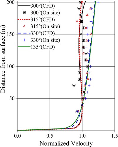
As discussed above, the prevailing wind direction at the site at a height of 200 m is between 300° and 330°. Figure 13 compares CFD and field measurement normalized longitudinal mean velocity profiles for several wind directions. The field measurement site data were randomly selected from windy periods (with a mean speed in excess of 10 m s⁻¹ at a height of 40 m) for the desired mean directions. All profiles are normalized by the velocity at a height of 40 m (bridge deck height). It can be seen that above a height of about 25 m the velocity profiles are fairly homogeneous, with only the profiles for directions of 135° and 330° showing a monotonic small increase with height. Overall, the CFD and field observation results show fairly good agreement.

Figure 13. Comparison of CFD and field measurement velocity profiles, normalized at a height of 40 m.

4.2. Spatial wind distribution

A dimensionless parameter K is defined herewith as the ratio of the local wind speed divided by the reference upstream velocity at the same height of 100 m, which can reveal terrain-induced effects visually. Figure 14 displays the wind speed ratio (K) contour. Note that color orange denotes a speed-up of about 1.0, red denotes a speed increase, and blue denotes a significant speed reduction. There are colored arrows showing the wind vector at the center of the bridge for four heights, scaled in magnitude to the reference wind speed shown by the red arrow. It is clear that the approach airflow direction has a remarkable effect on the airflow in the investigated area.

Figure 14. Wind velocity ratio at 100 m and spatial wind direction. (a) 270°. (b) 285°. (c) 300°. (d) 315°. (e) 330°. (f) 345°. (g) 360°. (h) 135°.

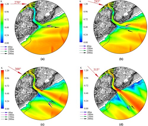
For wind directions of 270° and 285°, there are no speed-ups in the river valley but there are speed reductions in the leeward regions behind high ridges, which are sheltered from the approaching airflow. There are generally speed-ups in the valley exit region downstream of the approach wind direction. Thus, the areas with highest speed-ups move from east to west as the approaching airflow moves from 270° to 360°. The strongest speed-up occurs at 330° when the wind direction is aligned with the valley outlet direction. This indicates that the speed-up phenomenon is caused both by the approaching airflow direction as well as the zigzag river channel direction. The largest speed-ups are produced when the airflow is nearly parallel with the valley and the speed-up weakens when they become increasingly misaligned. It is notable that in the western corner of the zigzag river channel there is a calm spot with higher speeds in the inner (eastern) edge.

For the 135° direction corresponding to wind flow from the plain towards the mountains, the only region with speed-up is the entrance section of the valley, and the speed up there has a relatively low value. This indicates that the airflow can generate a stronger speedup when coming out the valley than into the valley.

The vertical variation of velocity is analysed by calculating velocity vectors at the field station location, as shown in Figure 14 where the results at 40, 100, 150, and 200 m are shown in different colors in the same scale, including the red vector showing the approach flow direction and speed. The velocity at 200 m is always closely parallel with the approach flow direction, whereas at lower heights the velocities show various amounts of rotation caused by terrain-induced effects. For 270° and 280°, as the height increases the wind directions rotate from being parallel with the mountain ridges to being the same as the approaching airflow direction. There is very little change in the wind direction with height for wind directions of 330°, 345° and 135° where the upper level wind direction is essentially parallel to the river valley.

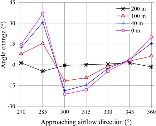
The direction changes are accurately quantified at the Sodar system location, and four lines showing the deviation in wind directions between the selected heights and the approach directions are presented in Figure 15. The small wind direction deviations are apparent at 200 m and the approaching flow direction of 345°. For the remaining cases, the wind direction deviations increase at progressively lower heights. The maximum deviation occurs for 285° where there is a huge twist in the flow direction of more than 40° between ground level and a height of 200 m. The results show that spatial wind direction is complicated by the combined effect of the approaching airflow direction and the terrain contour.

Figure 15. Deviation of wind directions with height from the approach direction, as a function of approach flow direction.

The important high-rise bridge tower structures are located in the expanding valley section, where the speed change with attitude is not necessarily a monotonic increasing trend as evidenced through wind speed vector length in Figure 14. Therefore, the vertical variation of the wind features at the tower locations are worthy of study. Figure 16(a,b) shows normalized velocity profiles at the two bridge towers obtained from the CFD study. The profiles are normalized using the upstream velocity at 100 m, i.e. they are K profiles.

Figure 16. (a) and (b) Velocity profiles at bridge towers A and B, (c) and (d) Surface streamlines and velocity vectors at bridge towers A and B. (a) Bridge tower A. (b) Bridge tower B. (c) 315 degrees. (d) 135 degrees.

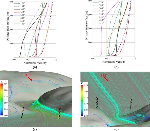
At bridge tower A location,all profiles (Figure 16(a)) show a speed up and the velocity profiles have typical power or log law shapes at directions 330° and 345°. Because of the sheltering effects of the hilly terrain for the other directions, their profiles show a range of shapes and a distinct speed reduction. There is even a speed reduction for the 315° direction because of the upstream hill on the western side of the river for this direction. Bridge tower B is located in a more exposed position directly in line with the narrowest section of the river valley (see Figure 3) further to the west, and as such, it experiences the strongest wind speeds from 315° and 330°. Clearly for the bridge, wind directions 315–330° are the most important for design as they are the highest, and they are also approximately normal to the bridge deck.

The airflow follows the terrain as shown in Figure 16(c,d). As the airflow comes out of the valley the streamlines spread out and diverge, but when airflow enters the valley the streamlines converge into the narrower region. The variation of the wind vectors with height is also displayed in Figure 16(c,d). It is easily observed from the results at 315° that the velocity vectors along tower A are spatially twisted from the local surface streamline towards the approaching airflow direction. There is no direction change over the height of tower B. However, for approach flow at 135°, it can be observed that, as expected, the velocity vectors along each tower are rotated towards the valley entrance.

4.3. Span-wise wind characteristics along the bridge deck

Figure 17 shows the wind characteristics along the bridge axis. It is apparent that the span-wise results are non-homogeneous and change significantly for approach directions 285–330°. In Figure 17(a) it can be seen that the wind speed is lower at the western end, except for 330° when the highest speed is at the center. It can be seen that the horizontal profiles rotate clockwise from 300° to 330°, and the biggest difference occurs at 285° where the speed is much higher at the eastern end. The wind speed from the plain (135°) is fairly homogeneous, as expected, since there are no obstructions upwind of the site for that direction.

Figure 17. Wind characteristics along the bridge axis. (a) Normalized wind velocity. (b) Wind inclination angle (positive = downwards). (c) Wind vectors for 315°approach flow. (d) Wind vectors for 135° approach flow.

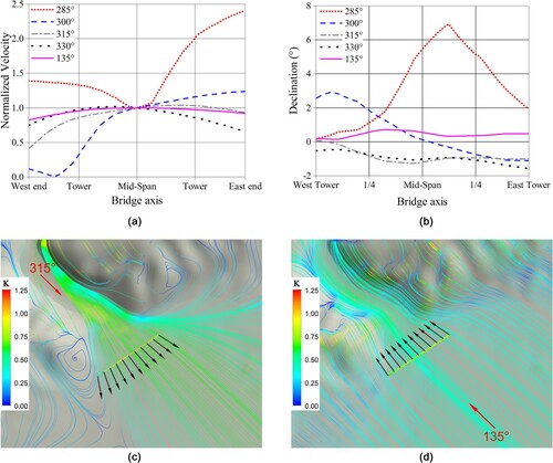
Figure 17(b) plots the inclination angle for the main span only. Although the bridge is built above a flat plain, there is small inclination angle in most cases. The maximum angle occurs when the airflow comes from 285° and has a value around 7°. This is caused by the wind flow approaching the bridge down the upwind hill. Figure 17(c,d) shows the velocity vectors at points along the bridge axis. It is apparent that there is good agreement between the results and the surface streamlines. The flow spreads out of the valley for 315° and converges into the valley for 135°.

Notably, there are non-homogeneous wind characteristics in this complex terrain vertically for both bridge towers as well as horizontally along the bridge deck. This should be considered in wind load design, and appropriate formulas used to replace the traditional values for homogeneous terrain. For instance, bridge towers are in the sphere of the terrain-induced effect, and the distribution of wind directions can be modeled as a linear variation where the terrain affects the direction near the surface and at a height of 200 m it tends towards the approaching airflow direction and is uninfluenced by the complex terrain.

5. Comparison to national code

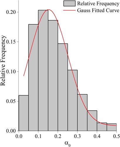
The Chinese Wind-resistant Design Specification for Highway Bridges  (JTG/T3360,2018/3360, 2018) specifies that the mean velocity profile should be described by the power-law formula according to Equation (6(6) $U(z)=k_f{\left(z╱10\right)}^{{\alpha }_0}{U}_{s10}$(6) ). (6) $U(z)=k_f{\left(z╱10\right)}^{{\alpha }_0}{U}_{s10}$(6) where U(z) is the reference wind speed at a height of z. U_s10 is the basic wind speed at the bridge site, defined as the 10-min wind velocity at a height of 10 m. k_f corresponds to the mean recurrence period based on the risk zone division and the basic wind speed. The surface roughness power-law exponent α₀ is dependent on the surface roughness category and the mean value should be applied when there are two categories of surface roughness. For the present study, assuming k_f = 1.0, the recommended surface roughness exponent α₀ is therefore 0.17, which is obtained by calculating the mean value of categories A for the plain and C for the valley.

In order to compare the Chinese code recommendation for the velocity profile with the field observations, power-law exponents were estimated using the non-linear least squares method by separately fitting 10-min vertical velocity profiles that were measured using the Sodar system to power-law profiles. Figure 18 shows a histogram of the relative frequency of the power-law exponent, and a Gaussian fitted probability density function (PDF) for α₀. It is apparent that the distribution matches the Gaussian distribution with a mean value of 0.152.

Figure 18. Relative frequency of α₀ from power-law profiles fitted to 10-min mean Sodar measured profiles.

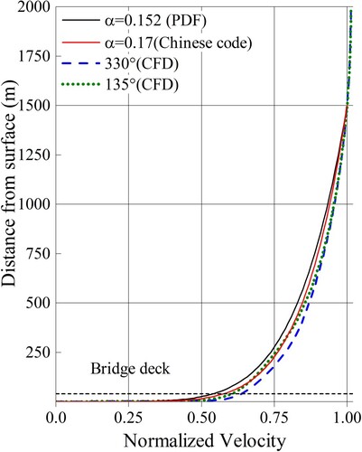
Considering that the mean velocity is essentially uniform above the gradient height of 1500 m, Figure 19 compares the normalized velocity profiles at the Sodar system location among the Chinese code, the field measurements and the CFD simulations with power-law-like results at the 135° and 330° directions. The ‘average’ Sodar profile (α = 0.152) at the bridge deck height is the smallest, as the field measurement wind speed results used in this fitting process were obtained without regard to wind direction. So the mean value of α only represents the majority situation, not the worst case. The profile recommended by the Chinese code is similar to the CFD result at the 135° direction, but lower than the result for the 330° direction. The difference between both CFD results is caused by the complex terrain. As-expected, the flow out of the valley generates a stronger speed-up. This means that the Chinese code only takes the terrain roughness into consideration, but loses sight of the topographic effects. The neglect of the topographic effects appears to induce an underestimated bridge reference wind speed, which could cause an unsafe design to proceed. Therefore, it is suggested that there should be a topographic variation factor in Equation (6(6) $U(z)=k_f{\left(z╱10\right)}^{{\alpha }_0}{U}_{s10}$(6) ), in order to take the terrain speed-up into account, when the code is used in the absence of other information such as wind tunnel tests of CFD studies.

Figure 19. Comparison of velocity profiles at the center of the bridge.

6. Conclusions

This paper presents the results of the study on wind characteristics of unusual terrain where there is a deep river valley on one side and a flat plain on the other side. The main conclusions are as follows:

1. The field measurement results show that the terrain-induced effects on the mean wind direction are more significant near the surface, resulting a slight rotation from west towards north with altitude and the wind characteristics at the two bridge towers are different because their upstream fetch is very complex.

2. Broad agreement between the on-site results and the CFD simulations indicates that the numerical method using the k–ε model is feasible for this complex terrain.

3. The wind direction has been shown to rotate from the valley direction to the onset flow direction over the height range of 200 m. The wind direction results along the road bed between the bridge towers were observed to vary in a linear fashion

4. The deep valley channel-like terrain generates speed-ups when the approaching airflow is aligned close to parallel with the valley. In the valley outlet area, a stronger speed up is generated when the airflow comes out of the valley compared to flowing into the valley.

5. The wind characteristics are non-homogeneous along the bridge deck and change in both approach wind direction and speed.

6. Chinese code recommends an underestimate for the wind speed, irrespective of the topographic variation. It is suggested that a correction factor for topographic effects is added into the reference equation.

Furthermore, the terrain-induced effects on the wind should be considered in the design loads when bridges are located in complex terrain like at this site. However, such cases are not addressed by the simplified rules in the codes, and as such, special studies must be undertaken to improve the applicability of the code, but also to provide more reliable reference wind speeds for the design of large, expensive and important structures such as bridges.

The performance of bridge structures under the action of non-homogenous wind characteristics will be investigated further in the future.

Disclosure statement

No potential conflict of interest was reported by the author(s).

Additional information

Funding

This work was supported by the National Natural Science Foundation of China [grant number 51978077].

References

- Blocken, B., Stathopoulos, T., & Carmeliet, J. (2007). CFD simulation of the atmospheric boundary layer: Wall function problems. Atmospheric Environment, 41(2), 238–252. https://doi.org/10.1016/j.atmosenv.2006.08.019
- Blocken, B., van der Hout, A., Dekker, J., & Weiler, O. (2015). CFD simulation of wind flow over natural complex terrain: Case study with validation by field measurements for Ria de Ferrol, Galicia, Spain. Journal of Wind Engineering and Industrial Aerodynamics, 147, 43–57. https://doi.org/10.1016/j.jweia.2015.09.007
- Celik, I. B., Ghia, U., Roache, P. J., Freitas, C. J., Coleman, H., & Raad, P. E.. (2008). Procedure for estimation and reporting of uncertainty due to discretization in CFD applications. Journal of Fluids Engineering, 130(7), 078001. https://doi.org/10.1115/1.2960953
- ESDU85020. (1985). Characteristics of atmospheric turbulence near the ground. Part II: Single point data for strong winds (neutral atmosphere). IHS (Global).
- Flay, R. G. J., King, A. B., Revell, M., Carpenter, P., Turner, R., Cenek, P., & Pirooz, A. A. S. (2019). Wind speed measurements and predictions over Belmont Hill, Wellington, New Zealand. Journal of Wind Engineering and Industrial Aerodynamics, 195, 104018. https://doi.org/10.1016/j.jweia.2019.104018
- Flay, R. G. J., & Stevenson, D. C. (1988). Integral length scales in strong winds below 20 m. Advances in Wind Engineering, 28, 21–30. https://doi.org/10.1016/B978-0-444-87156-5.50010-2
- Franke, J. (2007). Best practice guideline for the CFD simulation of flows in the urban environment. Meteorological Inst.
- Ghalandari, M., Shamshirband, S., Mosavi, A., & Chau, K. W. (2019). Flutter speed estimation using presented differential quadrature method formulation. Engineering Applications of Computational Fluid Mechanics, 13(1), 804–810. https://doi.org/10.1080/19942060.2019.1627676
- Hargreaves, D. M., & Wright, N. G. (2007). On the use of the k– model in commercial CFD software to model the neutral atmospheric boundary layer. Journal of Wind Engineering and Industrial Aerodynamics, 95(5), 355–369. https://doi.org/10.1016/j.jweia.2006.08.002
- JTG/T3360-01-2018. (2018). Wind-resistant design specification for highway bridges. Part 4: Wind parameters (pp. 15–24). Ministry of Communications of the People’s Republic of China.
- Little, C. G. (1969). Acoustic methods for the remote probing of the lower atmosphere. Proceedings of the IEEE, 57(4), 571–578. https://doi.org/10.1109/PROC.1969.7010
- Pirooz, A. A. S., & Flay, R. G. J. (2018). Comparison of speed-up over hills derived from wind-tunnel experiments, wind-loading standards, and numerical modelling. Boundary-Layer Meteorology, 168(2), 213–246. https://doi.org/10.1007/s10546-018-0350-x
- Pirooz, A. A. S., Flay, R. G. J., & Jahani, B. (2019, September 1-6). Wind flow over complex terrain: Comparison of RANS and hybrid RANS/LES simulations. The 15th International Conference on Wind Engineering, Beijing, China.
- Raithby, G. D., Stubley, G. D., & Taylor, P. A. (1987). The Askervein Hill project: A finite control volume prediction of three-dimensional flows over the hill. Boundary-Layer Meteorology, 39(3), 247–267. https://doi.org/10.1007/BF00116121
- Richards, P. J., & Hoxey, R. P. (1993). Appropriate boundary conditions for computational wind engineering models using the k-ε turbulence model. Journal of Wind Engineering and Industrial Aerodynamics, 46-47, 145–153. https://doi.org/10.1016/0167-6105(93)90124-7
- Richards, P. J., & Norris, S. E. (2011). Appropriate boundary conditions for computational wind engineering models revisited. Journal of Wind Engineering and Industrial Aerodynamics, 99(4), 257–266. https://doi.org/10.1016/j.jweia.2010.12.008
- Richards, P. J., & Norris, S. E. (2015). Appropriate boundary conditions for a pressure driven boundary layer. Journal of Wind Engineering and Industrial Aerodynamics, 142, 43–52. https://doi.org/10.1016/j.jweia.2015.03.003
- Salih, S. Q., Suliman, M., Rasani, M. R., Ariffin, A. K., & Yaseen, Z. M. (2019). Thin and sharp edges bodies-fluid interaction simulation using cut-cell immersed boundary method. Engineering Applications of Computational Fluid Mechanics, 13(1), 860–877. https://doi.org/10.1080/19942060.2019.1652209
- Song, J. L., Li, J. W., & Flay, R. G. J. (2020). Field measurements and wind tunnel investigation of wind characteristics at a bridge site in a Y-shaped valley. Journal of Wind Engineering and Industrial Aerodynamics, 202, 104199. https://doi.org/10.1016/j.jweia.2020.104199
- Vogt, S., & Thomas, P. (1995). SODAR—A useful remote sounder to measure wind and turbulence. Journal of Wind Engineering and Industrial Aerodynamics, 54-55, 163–172. https://doi.org/10.1016/0167-6105(94)00039-G