Aerodynamic damping and amplitude response of piezoelectric fans in free and confined space

ABSTRACT

The main objective is to develop a predictive model to directly predict and describe the sensitivity of aerodynamic damping and amplitude response to the proximity of surrounding walls. To achieve the objective of this study, the instantaneous fluid force loaded on the vibrating cantilever in free space and confined space are numerically studied. The correlation mechanisms between the unsteady flow characteristics and the aerodynamic damping are also discussed. It can be concluded that the fluid structure interactions can be attributed to the change in viscous damping when the vibrating cantilever approaches the solid wall. Based on Newton’s law of viscous fluid, a fluid flow model is developed to estimate the additional fluid force generated between the cantilever and the sidewall. The new developed predictive model for aerodynamic damping and amplitude response are validated, and the results show that there is a good agreement with the experimental results. The developed model provides an important tool for the prediction of damping and amplitude to help implement piezoelectric fans in practical confined physical space.

KEYWORDS:

• Piezoelectric fans
• vibrating cantilevers
• aerodynamic damping
• flow structure interaction

Nomenclature

$a$	=	Coefficient
$A$	=	Amplitude, mm
$A1$, $B1$	=	Odd Fourier series coefficient
$A_{\text{area},i}$	=	Facet area, m2
$C$	=	Width of the piezoelectric fan, mm
$Cf$	=	Modal aerodynamic damping
${C_f}^{\mathrm{\prime }}$	=	Modal added aerodynamic damping
$Cs$	=	Model internal structural damping
$dt$	=	Time step, s
$f$	=	Frequency, Hz
$f_{\text{exact}}$	=	Richardson extrapolation
$K_s$	=	Modal damping
$k^{+}$	=	Non-dimensional turbulent kinetic energy
$L$	=	Total length of piezoelectric fan, mm
$L1$	=	Length of piezoelectric patch, mm
$M_f$	=	Modal added mass
$M_S$	=	Modal mass
$p_2$	=	Formal order of accuracy
$r$	=	Mesh refinement ratio
$t$	=	Time, s
$t_b$	=	Thickness of shim, mm
$t_p$	=	Thickness of piezoelectric patch, mm
$u$	=	Velocity vector, m/s
$u_{\tau }$	=	Friction velocity
$u^{+}$	=	Non-dimensional velocity
$w$	=	Displacement of the beam, mm
$X$	=	Amplitude of the approximate harmonic response, mm
$x,y,z$	=	Coordinate, mm
$y^{+}$	=	Non-dimensional wall distance
$\delta$	=	Sidewall gap, mm
$\psi$	=	Mode shape
${ϵ}^{+}$	=	Non-dimensional dissipation rate
$\omega$	=	Oscillation frequency
${\omega }^{+}$	=	Non-dimensional specific dissipation rate
$\mu$	=	Dynamic viscosity, Pa·s
${\tau }_w$	=	Wall shear stress
$\upsilon$	=	Kinematic viscosity
$\rho$	=	Density of shim, kg/m3
${\rho }_f$	=	Density of fluid, kg/m3
${\rho }_p$	=	Density of piezoelectric patch, kg/m3

1. Introduction

As the development of modern electronic technology, chips with higher integration and smaller package sizes are demanded to meet the requirement of various electronic devices. The piezoelectric fan has some favorable characteristics due to its small size, low power, noiseless, compact and light weight, and is very suitable for cooling the high-density assembly electronic device (Ma et al., 2017; Maaspuro, 2016; Oh et al., 2018; Stafford & Jeffers, 2017; Sufian et al., 2014). Cooling performance for implementing piezoelectric fans in a laptop and a cell phone enclosure were studied by Açıkalın et al. (2004). They concluded that piezoelectric fans could improve the heat transfer performance of stagnant regions in the laptop by increasing fluid mixing. In the cell phone enclosure, piezoelectric fan performed better than the natural convection heat sink.

Many works have studied the unsteady flow and cooling performance of the piezoelectric fans by analytical, numerical, and experimental methods (Açıkalın et al., 2004; Fairuz et al., 2014; Tan et al., 2014; Toda, 1979; Wait et al., 2007). A piezoelectric fan is mainly composed of a flexible cantilever beam. Wait et al. (2007) conducted experimental measurements on the flow field characteristics and the vibration behavior of piezoelectric fans at different resonance modes. Air is drawn in from one side and pushed upward and downward away from the fan cantilever. The vortex is generated at the tip of cantilever and then pushed away. Different flow patterns are produced at different resonance modes. As the mode number of piezoelectric fan increases, the power losses increase while the fluid flow and thrust decrease. The first resonance mode is generally used for piezoelectric fans (Toda, 1979; Wait et al., 2007). With the rapid development of advanced computational tools, Computational Fluid Dynamics (CFD) has been a powerful approach to obtain fluid flow in various geometries and systems (Fairuz et al., 2014; Ghalandari et al., 2019; Salih et al., 2019; Tan et al., 2014). Tan et al. (2014) and Fairuz et al., (2014) numerically studied the flow and cooling performance gained by a vibrating cantilever at various resonance modes and operating parameters. Results show that the bulk flow and convective heat transfer performance generated in first mode are better than those in second mode. The distance between the fan and the heat sink has a significant effect on the flow field and convective heat transfer. Kimber et al. (2007, 2008) experimentally studied the performance of the piezoelectric fan. They developed the predictive relationships to describe the bulk fluid flow and convective heat transfer performance. They also studied the sensitivity of the fan performance to these vibration characteristics and distance from target.

The performance of piezoelectric fan arrays was also investigated (Kimber & Garimella, 2009). Results show that the fan pitch has important effects on the cooling performance and the vibrating behavior of the cantilevers. For flexible cantilevers, the added mass and aerodynamic damping caused by the fluid are important factors that make the amplitude and frequency change. In order to provide insight into the sensitivity of the fluid flow to vibration behavior, Kimber, Lonergan et al. (2009), Kimber, Suzuki et al. (2009) experimentally measured the amplitudes of fans in air and vacuum respectively. The experiment results show that two adjacent fans are obviously affected by each other in air. However, there is no such fluid-structural coupling effect in vacuum. In vacuum, whether a fan or the fan array was placed, the amplitude response is always the same. When the structure is large and its vibration behavior is relatively insignificant (as a bridge), fluid viscosity and vortex can be ignored. However, for structures with large amplitudes, such as micro aerial vehicle wings and piezoelectric fans, the effects of fluid viscosity and vortex cannot be ignored. Non-negligible damping can be caused by vortex-shedding (Fu & Price, 1987; Graham, 1980; Sarpkaya, 1995). Eastman et al. (2012) studied the effects of installation details on the vibration characteristics of cantilever. The results show that the aerodynamic damping increases as the sidewall gap decreases. When the sidewall gap is greater than 20 mm, the influence of the sidewalls can be ignored. However, as the gap is reduced to 5 mm, the influence of surrounding walls increases significantly. When the gap is equal to 1 mm, the quality factor (Q-factor) decreases by about 35%. Since the damping is increased, more power is required to keep the amplitude constant (Kimber et al., 2007; Kimber, Lonergan et al., 2009; Kimber, Suzuki et al., 2009).

In this work, we are concerned with the influence of installation details on piezoelectric fan performance. The main objective is to develop a predictive model to directly predict and describe the sensitivity of aerodynamic damping and amplitude response to the proximity of surrounding walls. The unsteady flow characteristics are studied numerically and theoretically. A comprehensive predictive model for aerodynamic damping is established. In addition, a method for predicting the amplitude of fan cantilever in confined physical space is developed. The correlation mechanisms between the unsteady flow characteristics and the aerodynamic damping are also discussed. Understanding the influence of installation details provides an important tool to help implement piezoelectric fans in practical confined physical space.

2. Model description

2.1. Geometry description

In order to reveal the three-dimensional unsteady fluid flow around piezoelectric fan, the CFD (Computational Fluid Dynamics) modeling and simulations are carried out. The numerical simulations consider two different surrounding walls arrangements, as shown in Figure 1. Figure 1(a,b) illustrates the numerical models of piezoelectric fans in the free space and the confined space, respectively. In Figure 1(a), the domain of free space has the dimensions of 100 mm × 100 mm × 100 mm. The six boundaries of the free space are set as open boundaries, similar to those in the literature (Açıkalın & Garimella, 2009). In Figure 1(b), two sidewalls are placed on both sides of the cantilever, as well as the other four boundaries are set as open boundaries. Both sidewalls have dimensions of 100 mm × 100 mm. The gap between the cantilever edge and the sidewall is $\delta$.

Figure 1. Schematic diagram of the numerical model, (a) Piezoelectic fan in free space, (b) Piezoelectric fan in confined space.

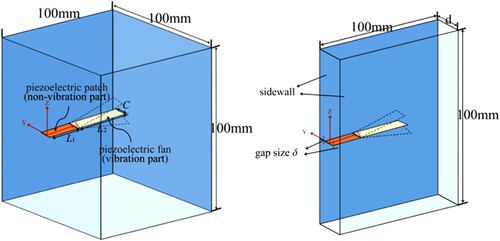
In order to simplify the numerical mesh, the zero thickness fan cantilever is established. Although the actual fan is driven by attached piezoelectric patch, the displacement of the patched part is significantly smaller than that of the unpatched part. So the displacement of piezoelectric patch is ignored. The total length and width of the fan cantilever are $L$ and $C$. The piezoelectric patch is of length $L_1$. The geometric and material properties are shown in Table 1.

Table 1. Geometric and material properties of the piezoelectric fan.

Physical quantity (units)	Symbol	Properties
Length of the piezoelectric patch (mm)	$L_1$	28.3
Length of the fan (mm)	$L$	64.9
Width of the fan (mm)	$C$	12.6
Thickness of the shim (mm)	$t_b$	0.25
Thickness of the piezoelectric patch (mm)	$t_p$	0.55
Density of the shim (kg/m^3)	$\rho$	1400
Density of the piezoelectric patch (kg/m^3)	${\rho }_p$	7800

2.2. Governing equations and boundary conditions

Numerical simulations for the 3D unsteady flow caused by cantilever are carried out by using commercial software package ANSYS FLUENT. The simulations include two coupled contents: (1) solving the unsteady flow field and (2) updating the deformation of the vibrating cantilever.

Firstly, an unsteady flow field can be obtained by solving the 3D unsteady RANS (Reynolds-averaged Navier-Stokes) equations. According to the previous works (Açıkalın & Garimella, 2009; Jang & Lee, 2014; Li et al., 2018; Lin, 2012), the results gained by the simulation studies with the SST k-ω model are the most consistent with the measurements. In the following section, the SST k-ω turbulence model is applied to calculate the turbulent viscosity. Second-order upwind scheme, SIMPLE scheme and the air properties are applied for simulations. As shown in Figure 1(a), the left boundary (next to the piezoelectric patch) of the free space is defined as an ambient-pressure inlet, and the other 5 boundaries are defined as ambient-pressure outlet. The cantilever surface is defined as a non-slip wall boundary. As shown in Figure 1(b), except the two sidewalls of the confined space model that are defined as non-slip wall boundaries, the other boundaries are the same as those of free space model. In this work, the length and width of the vibrating cantilever are 36.6 and 12.6 mm respectively. The cantilever vibrates at its natural frequency (f) of 60 Hz. Its amplitude (A) is 3.25 mm. The corresponding maximum tip speed $(u_{\text{tip}}=\omega \cdot A)$ and the oscillating Reynolds number ($\rho \cdot u_{\text{tip}}\cdot A/\mu$, according to Kim et al., 2004) are 1.22 m/s and 272, respectively.

Secondly, in order to describe the deformation of the vibrating cantilever, the equations representing the mode shape of the cantilever are described as follows: (1) $\begin{array}{rl}z\left(x,t\right)& =z_0\left(x\right)\sin \left(2\pi f\times t\right)\end{array}$(1) (2) $\begin{array}{rl}{z}_0\left(x\right)& =A\psi \left(x\right)\end{array}$(2) (3) $\begin{array}{rl}\psi \left(x\right)& =a{e}^{bx}-c\end{array}$(3) where $\psi \left(x\right)$ is the mode shape of the cantilever normalized by the maximum (tip) vibration amplitude $A$. $x$ is the coordinate. 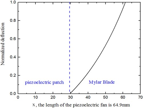For the piezoelectric fan considered in the present simulations, the constants in Equation (3) have the values: $a\text{ = 0}\text{.595486}$, $b\text{ = 1}\text{.083650}$, $c\text{ = 0}\text{.625384}$, referring to the works by Eastman et al. (2012). The mode shape $\psi \left(x\right)$ is provided in Figure 2. The displacements are relatively small in the piezoelectric patch region due to its greater stiffness. In the blade region, the mode shape is similar to a standard cantilever beam. $z\left(x,t\right)$ describes the periodic movement of the cantilever. $f$ is the frequency and $t$ represents time. The moving wall boundary is applied to the cantilever. The displacement of each point along the cantilever at every instant is defined by a UDF (User Defined Function) implemented in FLUENT.

Figure 2. Mode shape of piezoelectric fan normalized by the amplitude.

2.3. Grid generation and time-step

In order to identify and describe the position and deformation of the vibrating cantilever at every instant, dynamic mesh technology is needed. Dynamic mesh scheme includes the local remeshing and the smoothing method. The smoothing method models the grids motion as a spring. When the size of the deformed grid is too small or the skewness is too high, the remeshing method is applied. To improve the resolution of the boundary layer, a denser structured grid was constructed in the region adjacent to surface of vibrating cantilever and sidewalls. A systematic mesh sensitivity test shows that about 3.5 million cells (for the numerical model with free space, as shown in Figure 1(a)) can be adopted for the presented simulations. The computational domain of the confined space model with gap of 1 mm ($\delta =1\text{mm}$, as shown in Figure 1(b)) was meshed using the 1.4 million cells. The grid independence, near-wall flow characteristics (velocity, turbulent kinetic energy, dissipation rate, non-dimensional wall distance, et al.) and accuracy of near wall flow simulation are studied below, respectively.

It is necessary to use a small time step to accurately reveal the characteristics of unsteady flow in the present numerical simulation. When the frequency is 60 Hz and a cycle contains 200 time steps, the time step $dt$ can be expressed as Equation (4). (4) $dt=\frac{1\text{s}}{60\text{ cycles}}\times \frac{1\text{ cycles}}{\text{200}\text{ time steps}}$(4)

The Courant number, defined as Equation (5), gives the number of grids that the fluid passes through in a time step. In this work, the range of Courant numbers is 1–10. (5) $\text{Courant number}=\frac{\text{Characteristic flow velocity}\times dt}{\text{Typical cell size}}$(5)

An objective of the present work is to quantify the fluid force acting on piezoelectric fan. The unsteady flow simulation must be conducted for sufficient periods to obtain converged fluid force. Based on numerical simulation results, the fluid force acting on the cantilever is computed by the integration of surface pressure. (6) $F_m\left(t\right)=\int p_f\left(t\right)dS=\sum _{i=1}^{nf}{p}_{fi}\left(t\right)\cdot A_{\text{area},i}$(6) where $A_{\text{area},i}$ and $p_{fi}\left(t\right)$ are the facet area and the facet pressure on the cantilever, respectively.

In order to gain converged results, 20 periods are required for the simulation of the free space model, and 15 periods are required for the simulation of the confined space model in this work.

The grid independence is tested to ensure that the maximum deviation between fluid force values was less than 5%. The grid system of the free space model is considered here as an example. The coarse, medium, and fine grid system of the deforming domain contain 1.4, 2.4 and 3.3 million cells. The coarse, medium, and fine grid system of stationary domain contains 0.6, 1.1 and 1.2 million cells. The cell numbers of the whole domain are about 2.0, 3.5, and 4.5 million, respectively. As shown in Table 2, the fluid force acting on the vibrating cantilever (when the amplitude is 3.25 mm) is selected as the variable $f_i$ (i = 1, 2, 3 represent the fine, medium and coarse grid system, respectively). The relative discretization error (RDE) (Roy, 2005) is expressed as (7) $\begin{array}{rl}\text{RD}{\text{E}}_i& =\frac{1}{r^{p_2}-1}\cdot \frac{|f_i-f_{\text{exact}}|}{f_{\text{exact}}}\end{array}$(7) (8) $\begin{array}{rl}{f}_{\text{exact}}& =f_1-\frac{f_2-f_1}{r^{p_2}-1}\end{array}$(8) where $r$ is mesh refinement ratio $(r=r_{12}=1.4)$, $p_2$ is formal order of accuracy ($p_2=2$, in this work). $f_{\text{exact}}$ is obtained from Richardson extrapolation (expressed in Equation (8)). As shown in Table 2, the relative discretization error for all grid systems is no more than 5.0%. Considering the computing time and accuracy, the medium mesh is selected for further investigation.

Table 2. Grid convergence tests for the free space model.

Mesh	Fluid force (×10^−6N)
Fine mesh (4.5 million)	1510
Medium mesh (3.5 million)	1513
Coarse mesh (2.0 million)	1525
Extrapolation	1507
$RD{E}_i$ (%)	0.3
	0.5
	1.3

In addition, the minimum resolution of the mesh is studied, especially the effect of elements number across the gap is analyzed. The grid system of the confined space model with gap of 1 mm $(\delta =1\text{mm)}$ is considered here as an example. The structured mesh is developed at the vicinity of the walls with the $y^{+}<1$. The coarse, medium, and fine grid system contain 24, 34, and 48 elements across the gap. The cell numbers of the whole domain are about 1.2, 1.4, and 1.7 million respectively. For the three grid systems, the calculated values of the fluid force acting on the vibrating cantilever are obtained as shown in Figure 3. The corresponding numerical uncertainty, as computed using the Richardson extrapolation method (Roy, 2005) is shown in Table 3. It can be seen that the relative discretization error for all grid systems is no more than 5.0%. Considering the computing time and accuracy, the medium mesh $(y^{+}\approx 0.3)$ is selected for further investigation.

Figure 3. Comparison of the numerical fluid force loaded on the cantilever with different grid sizes.

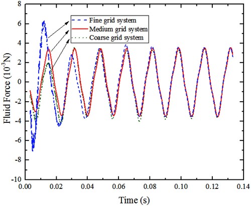
Table 3. Grid convergence tests for confined space model.

Mesh	Fluid force (×10^−6N)
Fine mesh (1.7 million)	3510
Medium mesh (1.4 million)	3545
Coarse mesh (1.2 million)	3629
Extrapolation	3474
$RD{E}_i$ (%)	1.1
	2.1
	4.6

3. Results and discussions

In this simulation, the cantilever is operated at the first resonance mode. Its frequency and amplitude are 60 Hz and 3.25 mm. The deformation of the vibrating cantilever at every instant is calculated according to Equations (1)–(3). Initial pressure in the fluid domain is set to ambient pressure, and initial speed is set to zero.

3.1. Instantaneous flow analysis

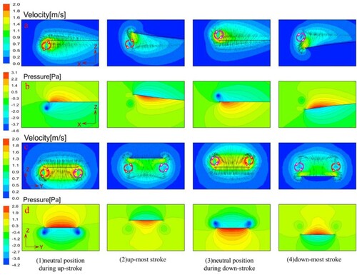
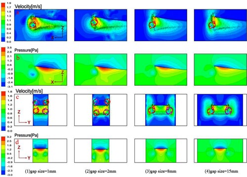
As the cantilever vibrates periodically, both the velocity and the pressure of fluid vary periodically over time. Figure 4 shows the velocity vector and pressure fields formed when the vibrating cantilever is at the typical positions. As shown in Figure 4(1-a, 1-b), the cantilever is initially at the undeflected position and is traveling upwards, forcing the fluid to displace rapidly. It can be seen that a low pressure region and a counter-clockwise vortex are generated under the tip of the cantilever. Simultaneously, a pair of vortices rotating in opposite directions are generated under both sides of the cantilever, as shown in Figure 4(1-c, 1-d). As shown in Figure 4(2), the cantilever reaches the extreme position upwards. Those vortices are forced away from the cantilever. In addition, those vortices have been weakened, and the pressure near the vortex core has decreased. The vortices and static pressure distribution around the cantilever have great effects on each other. As the cantilever is traveling downwards, the clockwise vortex is generated above the tip of the cantilever, as shown in Figure 4(3,4). Simultaneously, a pair of vortices rotating in opposite directions are generated above both sides of the cantilever. As the cantilever vibrates, vortices are generated and then forced upward or downward alternately.

Figure 4. Velocity and pressure distribution during a cycle (piezoelectric fan in free space).

3.2. Effects of sidewalls on the flow field

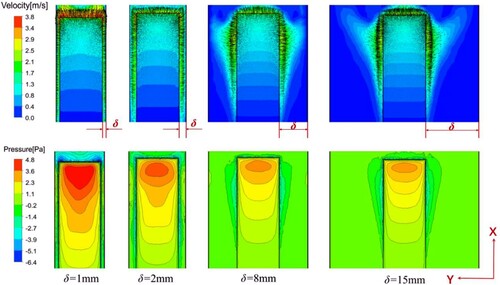
In this section, the effects of the sidewalls on the fluid flow caused by cantilever are discussed. The cases with different gaps between the sidewalls and the cantilever are numerically studied. Figure 5 shows the velocity vector and pressure fields formed when the cantilever reaches the extreme position upwards. As the sidewall gap is reduced, the influence of the sidewalls on the fluid flow becomes stronger, especially when the gap is smaller than 3.0 mm. When the gap is large enough, such as 8 and 15 mm, the sidewalls have little effects on the flow characteristics, which is consistent with the free space (as shown in Figure 4). When the gap is reduced to 1 mm, the influence of the sidewall becomes significant. In Figure 5(1-c), as the cantilever is traveling upwards, a pair of vortices rotating in opposite directions are generated under both sides of the cantilever, and a pair of vortices are also generated above the cantilever. Due to the effect of the side wall, the intensity of the vortices becomes stronger, and the static pressure around the cantilever becomes higher.

Figure 5. Velocity and pressure distribution during a cycle (piezoelectric fan in confined space).

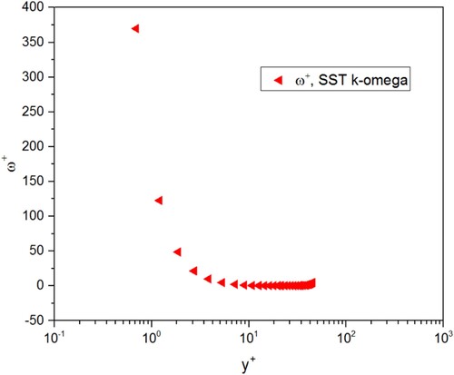
Turbulent flows are significantly affected by walls. In order to explain this behavior, near-wall flow characteristics are analyzed. Figures 6–9 show the non-dimensional variables ($u^{+}$, $k^{+}$, ${ϵ}^{+}$ and ${\omega }^{+}$) versus non-dimensional wall distance $y^{+}$ plots for the cantilever tip-to-wall region. $u^{+}$, $k^{+}$, ${ϵ}^{+}$, ${\omega }^{+}$ and $y^{+}$ are non-dimensional velocity, turbulent kinetic energy, dissipation rate and specific dissipation rate and non-dimensional wall distance respectively, defined as follows: $u^{+}=\frac{u}{u_{\tau }}$, $k^{+}=\frac{k}{u_{\tau }^2}$, ${ϵ}^{+}=\frac{ϵ}{\frac{u_{\tau }^4}{\upsilon }}$, ${\omega }^{+}=\frac{ϵ}{{\text{β}}^{\ast }k}$, $y^{+}=\frac{u_{\tau }y}{\upsilon }$. Where $u_{\tau }=\sqrt{\frac{{\tau }_w}{\rho }}$ is friction velocity, ${\tau }_w$ is wall shear stress, $\upsilon$ is kinematic viscosity respectively and ${\text{β}}^{\ast }=0.09$.

Figure 6. Near-wall non-dimensional velocity (u⁺) versus non-dimensional wall distance (y⁺).

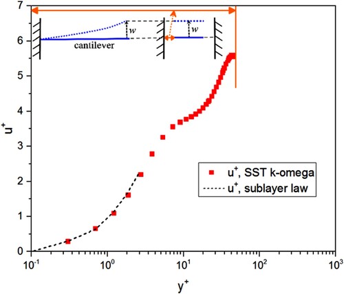
Figure 7. Near-wall non-dimensional turbulent kinetic energy (k⁺) versus wall distance (y⁺).

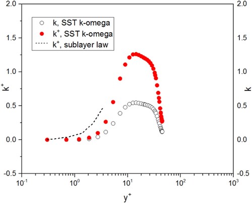
Figure 8. Near-wall non-dimensional dissipation rate (ϵ⁺) versus wall distance (y⁺).

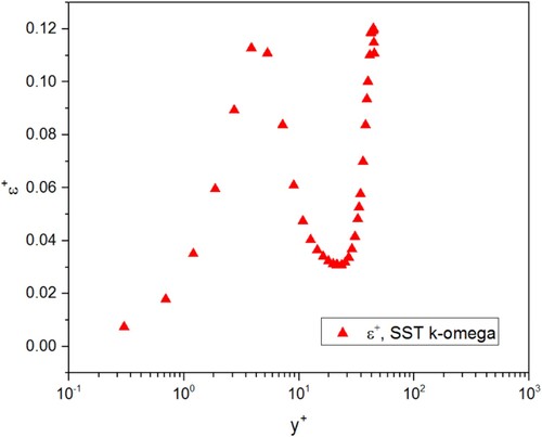
Figure 9. Near-wall non-dimensional specific dissipation rate (ω⁺) versus wall distance (y⁺).

As shown in Figure 6, the velocity reaches maximum near the cantilever tip. The near-wall velocity is affected through the no-slip condition that has to be satisfied at the wall. Near the wall $y^{+}<5$, called the viscous sublayer, the flow is laminar and the shear stress is nearly constant (Wilcox, 1998). In this region of viscous sublayer, the non-dimensional velocity profile can be expressed as: (9) $u^{+}=y^{+}$(9)

Figure 6 presents the predicted velocity profile (from this work) and the velocity profiles (from Equation (9), sublayer law). It can be seen that the predicted velocity profile in the viscous sublayer region is consistent with the sublayer law (Equation (9)). Figure 7 shows the non-dimensional turbulent kinetic energy $k^{+}$ versus non-dimensional wall distance $y^{+}$. The near-wall behavior of predicted turbulent kinetic energy $k^{+}$ is close to the sublayer law (Equation (10)) (10) $k^{+}=0.05y^{+2}$(10)

Toward the outer part of the near-wall region, turbulence kinetic energy rapidly increases due to the large velocity gradients. As shown in Figures 8 and 9, it can be seen that the dissipation rate is large where the production of turbulence kinetic energy is large.

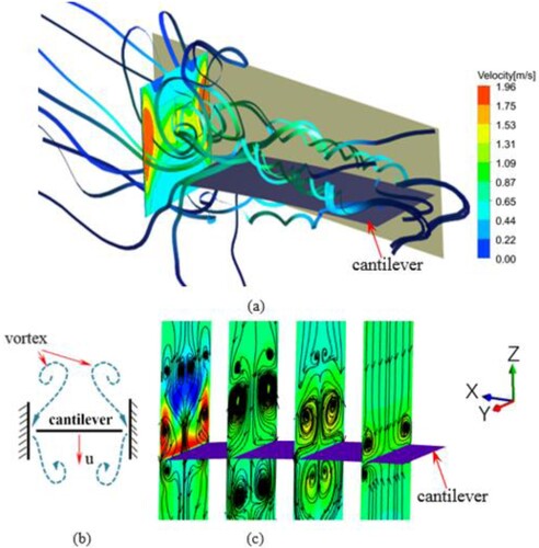
A good CFD mesh needs to capture the important vortex structures and produce accurate results. In this works, flow rotates creating vortices as it sheds off the cantilever surface, as shown in Figure 10. The development of major side-edge vortices is affected by the vibration amplitude (A), the width of cantilever (C) and the width of gap $\left(\delta \right)$. It can be seen from Figure 10 that the vortex scale is larger than $\delta$ and smaller than $C/2$. In order to establish the best mesh, we progressively increase the mesh density around areas of interest. The structured mesh is developed at the vicinity of the walls with the $y^{+}<1$. The grid system contains 34 elements across the gap ($\delta =1\text{mm}$ is considered here as an example). As shown in Figure 10, the major vortices structures have been captured with this grid system. There are enough elements modeling the vortices reducing numerical dissipation of the flow structure.

Figure 10. Streamlines and velocity contour distribution (cantilever reaches extreme position downwards).

4. Development of the theoretical model

4.1. Characteristics of the transient fluid force

4.1.1. In free space

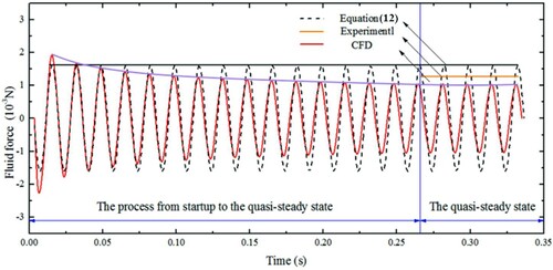
Figure 11 shows the instantaneous fluid force loaded on the vibrating cantilever, as it cycles through multiple oscillations. In Figure 11, the results of the present simulations are compared with the results of the literature (Bidkar et al., 2009). Bidkar et al. (2009) developed the predictive relationships (Equation (11)) to describe the separation of flow and the aerodynamic damping caused by vortex shedding. (11) $\begin{array}{rl}{F}_f\left(x,t\right)& =-{\rho }_f{A}^2|\psi \left(x\right)|\psi \left(x\right){\omega }^{2}C[A_1\cos (\omega t)\\ & +B_1\sin \left(\omega t\right)]\end{array}$(11)

Figure 11. Comparison of the theoretical, numerical and experimental fluid force loaded on the cantilever (A = 2.5 mm).

The fluid force $F_f\left(x,t\right)$ is a function of the axial location $x$ and the time $t$. ${\rho }_f$ is the fluid density. $\omega$ is oscillation frequency. $A_1$ and $B_1$ are the odd Fourier series coefficient (Keulegan & Carpenter, 1958). In Equation (11), $F_f\left(x,t\right)$ represents the fluid force per unit length of the cantilever. We use Equation (12) to obtain the total fluid force. (12) $F_{For,f}\left(t\right)={\int }_{L_1}^L{F}_f\left(x,t\right)dL$(12) where $L$ is the length of the cantilever.

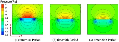
As shown in Figure 11, the CFD results show that the fluid force loaded on the vibrating cantilever varies periodically and develops to a quasi-steady state after multiple oscillations. Figure 4 shows the instantaneous pressure field. However, the theoretical results (from Equation (12)) and experimental results (Bidkar et al., 2009) are only obtained in the quasi-steady state. When the cantilever begins to vibrate (in the first period, 1 T), the fluid flow around cantilever begins to deforming. The vortices grow bigger and bigger until the fifteenth cycle (15 T). There is almost no difference in the fluid field between 15 and 20 T. It is interesting to note that the fluid force loaded on the cantilever at the beginning of the calculation (1 T) is largest. The fluid force becomes smaller and smaller until it reaches the quasi-steady state (15 T). In addition, as shown in Figure 12, the pressure around the cantilever gradually decreases with time. The development of fluid force during 40 cycles was recorded. The result shows that the quasi-steady state is reached after 20 cycles. In order to gain converged results, 20 periods are required for the simulation of the free space model in this work.

Figure 12. The static pressure around the cantilever.

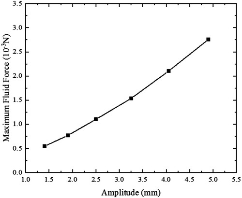
The numerical results of the maximum fluid force from the same cantilever vibrating at different amplitudes are shown in Figures 13 and 14. It can be seen that the fluid force increases as the vibration amplitude increases. In addition, a quasi-linear relationship between the fluid force and the oscillation amplitude can be clearly observed.

Figure 13. The maximum fluid force relation with the amplitude.

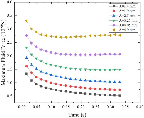
Figure 14. A quasi-linear relationship between the fluid force and the oscillation amplitude.

4.1.2. In confined space

In this section, the effects of the sidewalls on the instantaneous fluid force acting on the vibrating cantilever are studied. The fluid flow reaches the quasi-steady state faster in confined space than in free space. In particular, it can be seen in Figures 15 and 16 that the sidewalls have very significant effects on the fluid force when the gap is smaller than 5 mm. And the effects of the sidewalls can be ignored when the gap is about 15 mm. These results are similar to the experimental results in the literature (Eastman & Kimber, 2014).

Figure 15. The effects of the sidewalls on the instantaneous fluid force loaded on the cantilever (A = 3.25 mm).

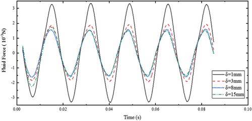
Figure 16. The fluid force relation with the gap size.

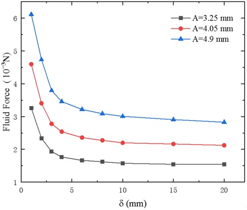
Figure 17 shows the effects of the sidewalls’ gap on both the velocity and fluid pressure. It can be concluded that the development of the side-edge vortices induced by the cantilever is seriously affected by the side-walls, as the gap $\left(\delta \right)$ between the cantilever and the side-wall becomes smaller. Moreover, as the $\delta$ becomes smaller, the velocity gradient between the cantilever and the sidewalls becomes obviously larger and the walls friction increases. So the fluid structure interactions can be attributed to the change in viscous damping. The trend can be expressed as the reduction of the gap causes the increase of fluid force acting on the vibrating cantilever.

Figure 17. Velocity and pressure distribution for each sidewall gap distance.

4.2. Description of the fluid force operator

The focus of the present work is to quantify the aerodynamic damping affected by the sidewalls. An accurate theoretical model for predicting aerodynamic damping can be a valuable tool for optimizing the installation details such as sidewalls.

The fluid force loaded on the vibrating cantilever is mainly determined by the operating parameters including the cantilever geometry and vibration amplitude and frequency. So the fluid force $F_{\text{fside}}\left(x,t\right)$ affected by a sidewall can be described in the following form: (13) $F_{\text{fside}}\left(x,t\right)=f\left(\delta ,A,\omega ,C,L,\cdots \right)$(13) where $\delta$, $A$, $\omega$, $C$ and $L$ express the sidewall gap, amplitude, frequency, width and length of the cantilever, respectively. The Equation (13) can be simplified as: (14) $F_{\text{fside}}\left(x,t\right)=f\left(\delta ,A,\omega ,g\right)$(14)

The relation of fluid force $F_{\text{fside}}\left(x,t\right)$ and the parameters $\delta$, $A$, $\omega$ is nonlinear. The $g$ factor represents the geometric parameters of the cantilever.

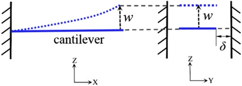
As shown in Figures 15–17, the sidewalls have very significant effects on the fluid flow when the gap is smaller than 5 mm. Especially, it can be seen in Figure 17 that the velocity gradient between the cantilever and the sidewalls is obviously larger when the gap is 1 and 2 mm. And this will directly cause greater viscous resistance. So based on Newton’s law of viscous fluid, the additional fluid force generated between the cantilever and the sidewall can be described as (15) $F_{\text{fside}}\left(x,t\right)=a\mu {\frac{du}{dy}|}_{\left(x,t\right)}$(15) where $F_{\text{fside}}\left(x,t\right)$ is additional fluid force. $a$ is a coefficient related to geometric parameters, $\mu$ is dynamic viscosity coefficient, and $\frac{du}{dy}$ is the velocity gradient between the cantilever and the sidewall. The $x$, $y$ and $z$ coordinate system is shown in Figure 18.

Figure 18. Coordinate of piezoelectric fan.

The displacement of the cantilever $w\left(x,t\right)$ is (16) $w\left(x,t\right)=A\psi \left(x\right)\cos \left(\omega t\right)$(16)

By noting that the velocity can be described as follows, (17) $\frac{d\left(w\left(x,t\right)\right)}{dt}=-A\psi \left(x\right)\omega \sin \left(\omega t\right)$(17)

Equation (17) is used to obtain the following description for $F_{\text{fside}}\left(x,t\right)$ (18) $\begin{array}{rl}{F}_{\text{fside}}\left(x,t\right)& =a\mu {\frac{du}{dy}|}_{\left(x,t\right)}=a\mu \frac{\left(-A\psi \left(x\right)\omega \sin \left(\omega t\right)\right)-0}{\delta }\\ & =\frac{-a\mu A\psi \left(x\right)\omega \sin \left(\omega t\right)}{\delta }\end{array}$(18) where $\delta$ is the gap between the cantilever edge and the sidewall.

Based on the mathematical description of fluid force of the piezoelectric fan in free-space, the fluid force of piezoelectric fan with the additional fluid force caused by sidewall in confined space is (19) $F\left(x,t\right)=F_f\left(x,t\right)+F_{\text{fside}}\left(x,t\right)$(19) $F_f\left(x,t\right)$ is described by Equation (11), and $F_{\text{fside}}\left(x,t\right)$ is described by Equation (18). The fluid force $F\left(x,t\right)$ represents the fluid force per unit length of the beam. We use Equation (20) to obtain the total fluid force (20) $F_{For,F}\left(t\right)={\int }_{L_1}^{L}F\left(x,t\right)dL$(20)

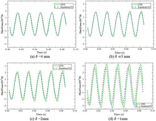
Figure 19 shows the predictions of Equation (20) and the CFD results of the instantaneous fluid force loaded on the vibrating cantilever. Overall, the model developed in this work is capable of predicting the fluid force in confined space. These theoretical trends and the sensitivity of fluid force are consistent with the numerical results.

Figure 19. The theoretically predicted and numerical fluid force for each sidewall gap distance.

4.3. Prediction method of amplitude in confined space

In order to predict the aerodynamic damping and the amplitude response, Bidkar et al. (2009) estimate a fluid force operator for harmonic motions of slender, sharp-edged beams. They also provide a general solution procedure for using single-mode Galerkin approximation to obtain the amplitude response. In the remainder of this section, we use the similar procedure to obtain the amplitude of cantilever oscillating in the confined space.

The cantilever motion is expressed in the form $w\left(x,t\right)=q\left(t\right)\psi \left(x\right)$, and the ordinary differential equation can be described as (21) $M_s\ddot{q}+C_s\dot{q}+K_{s}q=-M_f\ddot{q}-C_f\dot{q}-{C_f}^{\mathrm{\prime }}\dot{q}+F_{\text{modal}}\left(t\right)$(21) where $q\left(t\right)$ is the generalized coordinate, $\psi \left(x\right)$ is the mode shape and $\stackrel{\bullet }{\left(\right)}=\frac{d\left(\right)}{dt}$. $M_s$, $C_s$, $K_s$ and $F_{\text{modal}}\left(t\right)$ are structural modal mass, modal damping, modal stiffness and modal force. $F_{\text{modal}}\left(t\right)$ can be written as $F_{\text{modal}}\left(t\right)={F_{proj}}^{j\omega t}$. $M_f$ and $C_f$ represent the modal added-mass and the modal aerodynamic damping effects due to the surrounding air. In particular, ${C_f}^{\mathrm{\prime }}$ represents the modal aerodynamic damping effects due to the sidewalls. So $F_f\left(x,t\right)$ and $F_{\text{fside}}\left(x,t\right)$ can be used to describe the fluid force ($M_f\ddot{q}+C_f\dot{q}$ and ${C_f}^{\mathrm{\prime }}\dot{q}$) loaded on the cantilever in free space and confined space. Based on Equation (21), the amplitude of cantilever oscillating in the confined space can be given by: (22) $X=\frac{F_{\text{proj}}}{\sqrt{{\left(K_s-\left(M_s+M_f\right){\omega }^2\right)}^2+{\left(\left(C_s+C_f+{C_f}^{\mathrm{\prime }}\right)\omega \right)}^2}}$(22)

The followings are the comparisons of the predictions of Equation (22) with the experimental results by Bidkar et al. (2009) and Eastman and Kimber (2014). The piezoelectric fan considered in the present work is fabricated from mylar. The geometric and material properties are shown in Table 1. First, $M_s$, $C_s$, $K_s$ and $F_{proj}$ are estimated by using geometric, material properties and the in-vacuo amplitude response ($A=6.28\text{mm}$, $\omega =377$, according to Bidkar et al., 2009). $M_f$ and $C_f$ are calculated based on Equation (12). For free space (i.e. without sidewalls, ${C_f}^{\mathrm{\prime }}=0$), the theoretically predicted amplitude (by Equation (22)) of cantilever oscillating in air is 3.1 mm. The error in predicting the amplitude is about 5% (predicted value of 3.1 mm, and experimental value is 3.25 mm according to Bidkar et al. (2009). 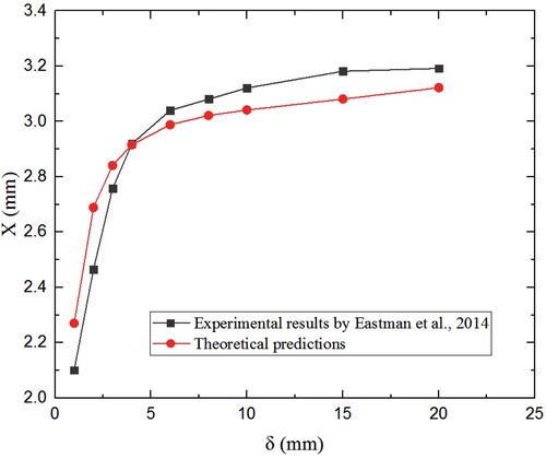Second, for confined space $({C_f}^{\mathrm{\prime }}\ne 0)$, the theoretically predicted amplitudes by Equations (20) and (22) of cantilever oscillating in air are shown in Figure 20. It can be seen that the sidewalls have very significant effects on the amplitude response when the gap is smaller than 5 mm. And the effects of the sidewalls can be ignored when the gap is about 15 mm. It is concluded that these theoretical trends and the sensitivity of amplitude response to sidewall gap are consistent with the experimental results in the literature (Eastman & Kimber, 2014).

Figure 20. The experimental (Eastman & Kimber, 2014) and theoretically predicted amplitude for each sidewall gap distance.

5. Conclusion

In this work, aerodynamic damping and amplitude response of oscillating cantilever in confined space are studied. Firstly, the instantaneous flow fields caused by cantilever are numerically studied. As the cantilever vibrates in free space (i.e. without sidewalls), vortices are generated and then forced upward or downward alternately. For confined space, the intensity of the vortices becomes stronger due to the effect of the sidewalls. It can be concluded that the fluid structure interactions can be attributed to the change in viscous damping when the vibrating cantilever approaches the solid wall. The trends can be expressed as the decrease of the sidewall gaps causes the increase of fluid force acting on the vibrating cantilever. Secondly, based on Newton’s law of viscous fluid, a fluid flow model is developed to estimate the additional fluid force generated between the cantilever and the sidewall. In addition, a general method is developed to predict the amplitude dependence of aerodynamic damping. The theoretical results show that the sidewalls have significant effects on the amplitude response when the gap is smaller than 5 mm. The effects of the sidewalls can be ignored when the gap is about 15 mm. These theoretical trends and the sensitivity of amplitude response to sidewall gap are consistent with the experimental results. Although the predictive model for aerodynamic damping and amplitude of the piezoelectric fan with sidewalls are obtained, there are many potential future works that can be deduced. Only a side-wall shape is analyzed in this work. However, there may be more effective sidewalls (as there are multiple possible orientations and numbers of sidewalls). A possible direction for future work is the extension of the current model to include the effects of various installation details.

Disclosure statement

No potential conflict of interest was reported by the author(s).

Additional information

Funding

This work was supported by State Key Laboratory of Mechanics and Control of Mechanical Structures (Nanjing University of Aeronautics and Astronautics) [grant number MCMS-E-0220G01].

References

- Açıkalın, T., & Garimella, S. V. (2009). Analysis and prediction of the thermal performance of piezoelectrically actuated fans. Heat Transfer Engineering, 30(6), 487–498. https://doi.org/10.1080/01457630802529115
- Açıkalın, T., Wait, S. M., Garimella, S. V., & Raman, A. (2004). Experimental investigation of the thermal performance of piezoelectric fans. Heat Transfer Engineering, 25(1), 4–14. https://doi.org/10.1080/01457630490248223
- Bidkar, R. A., Kimber, M., Raman, A., Bajaj, A. K., & Garimella, S. V. (2009). Nonlinear aerodynamic damping of sharp-edged beams at low keulegan-carpenter numbers. Journal of Fluid Mechanics, 634, 269–289. https://doi.org/10.1017/S0022112009007228
- Eastman, A., Kiefer, J., & Kimber, M. (2012). Thrust measurements and flow field analysis of a piezoelectrically actuated oscillating cantilever. Experiments in Fluids, 53(5), 1533–1543. https://doi.org/10.1007/s00348-012-1373-6
- Eastman, A., & Kimber, M. L. (2014). Aerodynamic damping of sidewall bounded oscillating cantilevers. Journal of Fluids and Structures, 51, 148–160. https://doi.org/10.1016/j.jfluidstructs.2014.07.016
- Fairuz, Z. M., Sufian, S. F., Abdullah, M. Z., Zubair, M., & Abdul Aziz, M. S. (2014). Effect of piezoelectric fan mode shape on the heat transfer characteristics. International Communications in Heat and Mass Transfer, 52, 140–151. https://doi.org/10.1016/j.icheatmasstransfer.2013.11.013
- Fu, Y., & Price, W. G. (1987). Interactions between a partially or totally immersed vibrating cantilever plate and the surrounding fluid. Journal of Sound & Vibration, 118(3), 495–513. https://doi.org/10.1016/0022-460X(87)90366-X
- Ghalandari, M., Koohshahi, E. M., Mohamadian, F., Shamshirband, S., & Chau, K. W. (2019). Numerical simulation of nanofluid flow inside root canal. Engineering Applications of Computational Fluid Mechanics, 13(1), 254–264. https://doi.org/10.1080/19942060.2019.1578696
- Graham, J. M. R. (1980). The forces on sharp-edged cylinders in oscillatory flow at low Keulegan-Carpenter numbers. Journal of Fluid Mechanics, 97(2), 331–346. https://doi.org/10.1017/S0022112080002595
- Jang, D., & Lee, K. S. (2014). Flow characteristics of dual piezoelectric cooling jets for cooling applications in ultra-slim electronics. International Journal of Heat and Mass Transfer, 79, 201–211. https://doi.org/10.1016/j.ijheatmasstransfer.2014.08.013
- Keulegan, G. H., & Carpenter, L. H. (1958). Forces on cylinders and plates in an oscillating fluid. Journal of Research of the National Bureau of Standards, 60(5), 423–440. https://doi.org/10.6028/jres.060.043
- Kim, Y. H., Wereley, S. T., & Chun, C. H. (2004). Phase-resolved flow field produced by a vibrating cantilever plate between two endplates. Physics of Fluids, 16(1), 145–162. https://doi.org/10.1063/1.1630796
- Kimber, M., & Garimella, S. V. (2009). Cooling performance of arrays of vibrating cantilevers. Journal of Heat Transfer, 131(11), 1314–1316. https://doi.org/10.1115/1.3153579
- Kimber, M., Garimella, S. V., & Raman, A. (2007). Local heat transfer coefficients induced by piezoelectrically actuated vibrating cantilevers. ASME Journal of Heat Transfer, 129(9), 1168–1176. https://doi.org/10.1115/1.2740655
- Kimber, M., Lonergan, R., & Garimella, S. V. (2009). Experimental study of aerodynamic damping in arrays of vibrating cantilevers. Journal of Fluids & Structures, 25(8), 1334–1347. https://doi.org/10.1016/j.jfluidstructs.2009.07.003
- Kimber, M., Suzuki, K., Kitsunai, N., Seki, K., & Garimella, S. V. (2008). Quantification of piezoelectric fan flow rate performance and experimental identification of installation effects. Conference on Thermal Thermomechanical Phenomena in Electronic Systems, 25(2), 1471–1474. https://doi.org/10.1109/ITHERM.2008.4544307
- Kimber, M., Suzuki, K., Kitsunai, N., Seki, K., & Garimella, S. V. (2009). Pressure and flow rate performance of piezoelectric fans. Transactions on Components and Packaging Technology, 32(4), 766–775. https://doi.org/10.1109/TCAPT.2008.2012169
- Li, X. J., Zhang, J. Z., & Tan, X. M. (2018). Experimental and numerical investigations on convective heat transfer of dual piezoelectric fans. SCIENCE CHINA Technological Sciences, 61(2), 232–241. https://doi.org/10.1007/s11431-017-9084-2
- Lin, C. N. (2012). Analysis of three-dimensional heat and fluid flow induced by piezoelectric fan. International Journal of Heat Mass Transfer, 55(11–12), 3043–3053. https://doi.org/10.1016/j.ijheatmasstransfer.2012.02.017
- Ma, H. K., Liao, S. K., & Hsieh, C. H. (2017). Development of a radial flow multiple magnetically coupled fan system with one piezoelectric actuator. International Communications in Heat and Mass Transfer, 87, 212–219. https://doi.org/10.1016/j.icheatmasstransfer.2017.07.018
- Maaspuro, M. (2016). Piezoelectric oscillating cantilever fan for thermal management of electronics and LEDs – A review. Microelectronics Reliability, 63, 342–353. https://doi.org/10.1016/j.microrel.2016.06.008
- Oh, M. H., Park, S. H., Kim, Y. H., & Choi, M. (2018). 3D flow structure around a piezoelectrically oscillating flat plate. European Journal of Mechanics/B Fluids, 67, 249–258. https://doi.org/10.1016/j.euromechflu.2017.09.002
- Roy, C. J. (2005). Review of code and solution verification procedures for computational simulation. Journal of Computational Physics, 205(1), 131–156. https://doi.org/10.1016/j.jcp.2004.10.036
- Salih, S. Q., Aldlemy, M. S., Rasani, M. R., Ariffin, A. K., Ya, T. M. Y. S. T., Ansari, N. A., Yaseen, Z. M., & Chau, K. W. (2019). Thin and sharp edges bodies-fluid interaction simulation using cut-cell immersed boundary method. Engineering Applications of Computational Fluid Mechanics, 13(1), 860–877. https://doi.org/10.1080/19942060.2019.1652209
- Sarpkaya, T. (1995). Hydrodynamic damping, flow-induced oscillations, and biharmonic response. Journal of Offshore Mechanics & Arctic Engineering, 117(4), 232–238. https://doi.org/10.1115/1.2827228
- Stafford, J., & Jeffers, N. (2017). Aerodynamic performance of a vibrating piezoelectric blade under varied operational and confinement states. Transactions on Components Packaging and Manufacturing Technology, 7(5), 751–761. https://doi.org/10.1109/TCPMT.2017.2666879
- Sufian, S. F., Fairuz, Z. M., Zubair, M., Abdullah, M. Z., & Mohamed, J. J. (2014). Thermal analysis of dual piezoelectric fans for cooling multi-LED packages. Microelectronics Reliability, 54(8), 1534–1543. https://doi.org/10.1016/j.microrel.2014.03.016
- Tan, L., Zhang, J. Z., & Tan, X. M. (2014). Numerical investigation of convective heat transfer on a vertical surface due to resonating cantilever beam. International Journal of Thermal Sciences, 80, 93–107. https://doi.org/10.1016/j.ijthermalsci.2014.02.004
- Toda, M. (1979). Theory of air flow generation by a resonant type PVF2 bi-morph cantilever vibrator. Ferroelectrics, 22(1), 911–918. https://doi.org/10.1080/00150197908239445
- Wait, S. M., Basak, S., Garimella, S. V., & Raman, A. (2007). Piezoelectric fans using higher flexural modes for electronics cooling applications. Transactions on Components and Packaging Technology, 30(1), 119–128. https://doi.org/10.1109/TCAPT.2007.892084
- Wilcox, D. C. (1998). Turbulence modeling for CFD. DCW Industries.