Numerical simulation of ball bearing flow field using the moving particle semi-implicit method

ABSTRACT

The distribution of lubricating oil in the bearing cavity is of great significance to bearing lubrication and cooling. A new idea is provided to further study the ball bearings lubrication, to achieve effective lubrication of bearings. The flow field of oil injection lubrication ball bearings is studied by the moving particle semi-implicit (MPS) method. The accuracy of the numerical calculation method is verified by experiments. The oil distribution of the bearing lubrication flow field and churning torque of the ball and cage at different speeds are analyzed. The research results show the maximum oil content in the bearing cavity is distributed in the range of about 90° to 120°. As the increase of rotating speed, the number of particles in the bearing cavity decreases. The churning torque decreases with the increase of rotating speed and increases with the increase of the oil viscosity. This study provides a new numerical calculation method for the lubrication flow field of ball bearings.

KEYWORDS:

• MPS method
• ball bearings
• oil-jet lubrication
• flow pattern
• churning torque

Nomenclature

Cs	=	Smagorinsky constant, -
d	=	The spatial dimension of the solution, -
dN	=	Nozzle diameter, mm
f	=	Body forces (per unit volume), N/m3
h	=	Effective radius, m
l	=	Width, mm
m	=	Particle mass, kg
ni	=	The rotational speed of the inner ring, r/min
ni	=	The particle number density, -
n0	=	Initial particle density, -
nm	=	Rotation speed of the balls and cage, r/min
p	=	Pressure, Pa
r	=	The distance between two particles, m
r	=	Displacement vector of particle, m
rb	=	Ball radius, mm
re	=	Finite space for limiting the interactions, m
rin	=	Inner radius, mm
rm	=	Pitch radius, mm
rout	=	Outer radius, mm
$\overline{S}$	=	Mean strain rate, -
t	=	Time, s
T	=	Oil temperature, °C
u*	=	Predicted velocity, m/s
u	=	Velocity vector, m/s
Z	=	Number of balls, -
∇	=	Gradient operator, -
∇2	=	Laplacian operator, -

Greek symbols

$\mathrm{\Delta }X$	=	Particle space, m
$\mathrm{\Delta }t$	=	Time step, s
α	=	Bearing contact angle, °
αc	=	Contact angle, °
θ	=	Wall contact angle, °
λ	=	The correction factor, -
μt	=	Turbulent viscosity coefficient, Ns/m2
ν	=	Kinematic viscosity, m2/s
ρ	=	Fluid density, kg/m3
σ	=	Surface tension coefficient, N/m
ϕ	=	Physical parameter of particle, -
ω	=	Kernel function, -

Subscript

i	=	Particle i
j	=	Particle j
virtual	=	Virtual particles

1. Introduction

In aircraft engines, motor spindles and drive trains, rolling bearings are widely used (Bossmanns & Tu, 1999; Fondelli et al., 2015; Gorse et al., 2006). Its operating performance is very crucial to the power performance and reliability of the whole transmission system (Gloeckner, 2013). In the automotive industry, power transmission is designed to achieve a higher speed (Nagaoka et al., 2015). The bearing will produce a lot of heat at high-speed. Therefore, effective and reasonable lubrication is very essential for high-speed bearings (Pang et al., 2008). Under the condition of high speed, the bearing temperature increases, which leads to bearing failure (Chang et al., 2017). It is of great significance to evaluate and improve the lubrication status of bearings by studying the distribution characteristics of the internal flow field of bearings under the condition of injection lubrication.

The flow field in the bearing cavity is relatively complex, and there is a strong interaction between the fluid and cage and roller (Gao et al., 2018). Some scholars have obtained the internal lubrication characteristics of bearings through experiments. An X-ray computed tomography (CT) imaging system was used to capture the grease distribution in a ball bearing and the internal grease flows (Noda et al., 2016). A specially designed test rig was established, and the flow field data were obtained by particle image velocimetry (PIV) technology (Lee et al., 2005). To study the impact of the oil supply flow rate and rotation speed on the oil distribution, Wu et al. built the bearing temperature and flow visualization test rig (Wu, Hu, Hu, et al., 2016). Aidarinis et al. (2011) established an experimental platform to test the change of the air-flow field in the bearing cavity. The lubricant fluid velocity field in the bearing was measured by the laser Doppler anemometry (LDA) system. It is not easy to test the flow field in the bearing cavity through experiments because the bearing structure is compact and the internal space is small. Computational fluid dynamics (CFD) method for the cooling flow inside the rolling element bearing was proposed. Bristot et al. (2016) used the CFD method to research the gas–liquid two-phase flow and the movement of the liquid droplet. Crouchez-Pillot and Morvan (2014) carried out numerical simulation calculations on the fluid field of bearing chamber in aero-engine, and adopted the volume of fluid (VOF) method and grid adaptive technology to track the flow field. Adeniyi et al. (2017) used the coupled level-set VOF (CLSVOF) method to calculate the lubrication flow field in the bearing cavity. It was found that the variation of the wetted area with shaft speed and the oil flow rate was inconsistent. Gao et al. employed the finite volume method(FVM) to compute the churning loss of roller bearings, and studied the distribution of oil and the change law of volume fraction with rotating speed (Gao et al., 2018; Gao, Lyu, et al., 2019). Then, Gao et al. also researched the distribution of lubricating oil under the bearing ring by CLSVOF multi-phase flow method (Gao, Nelias, et al., 2019). Wu and Hu et al. (Hu et al., 2014; Wu et al., 2017) studied the distribution of bearing oil volume fraction and temperature by VOF model and analyzed the influence of oil supply flow, speed and nozzle size on oil distribution and temperature. Yan et al. (2018) defined the rotating coordinates and established the lubrication flow field model of the bearing chamber. The visual flow field test scheme based on PIV technology for bearing chamber flow monitoring was proposed. The fluid distribution and vortex field in the bearing chamber were obtained.

All the above-mentioned researches mainly focused on bearing lubrication flow field with the Euler mesh method. When simulating the characteristics of the bearing lubrication flow field, the results are closely related to the type and quality of mesh generation. For complex geometry and steady and time-varying interacting loads, some results may be affected by the combination of grid modules and the flow information transfer mode. It not only dramatically adds a lot of calculation, but also increases the risk of error expansion and calculation instability.

In 1995, Koshizuka et al. (1995) proposed the MPS method for the first time. The MPS method is to divide the continuous fluid domain into a series of Lagrangian particles. The interaction between particles is realized through the integration of kernel function (1996). The advantage of the MPS method in numerical simulation is that compared with the traditional meshed CFD simulation method, it can save a lot of tedious work of mesh generation when dealing with the flow on the complex interface and large deformation flow on the free surface. Because of the flexibility, robustness and high efficiency of fluid analysis, the simulation of the complex flow field is close to the actual situation. For the past few years, the MPS method has been largely used in numerical calculation of marine engineering and mechanical engineering (Chen et al., 2020; Duan et al., 2017, 2018; Gotoh & Khayyer, 2018; Guo et al., 2020; Sun et al., 2017).

The description of the lubricant flow field distribution of bearing is of great significance to the prediction of bearing temperature. The application of an efficient and high-precision method of calculating bearing lubrication is of inestimable value to bearing optimization design. In this paper, the MPS numerical calculation method is applied to the distribution calculation of the bearing lubrication flow field. The flow field patterns associated with the oil injection lubrication at different speeds are studied. The aim is to propose a new method for calculating the flow field distribution of bearing lubrication.

2. System description

The drawing of the two-dimensional and three-dimensional structure of ball bearing jet lubrication is shown in Figure 1. Lubricating oil is sprayed from the nozzle to the bearing balls, cage, and inner and outer rings. The oil interacts strongly with the rotating balls, cage and inner ring.

Figure 1. Drawing of oil injection lubrication mechanism (a) Three-dimensional drawing (b) Two-dimensional drawing (Wu, Hu, Yuan, et al., 2016).

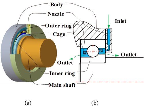
The type of angular contact ball bearing used in this experiment is SKF 7210 BECBP. The structural dimension parameters of the SKF 7210 BECBP are given in Table 1. The lubricating oil is an automatic transmission fluid, which is ATF DEXRON III. The parameters of lubricating oil are shown in Table 2. The spindle rotation causes the bearing inner ring to rotate, and the interaction force between the inner ring and the roller causes the roller and cage to move. The motion of the rolling elements will cause a complex flow of the lubricant oil. In the process of calculation, the rotational speed of bearing balls and cage needs to be determined. The formula for calculating the rotational speed of balls and cage was proposed by Harris and Kotzalas (2006). (1) $n_m=\frac{1}{2}{n}_i\left(1-\frac{r_b\cos \alpha }{r_m}\right)$(1) where n_i is the rotation speed of the inner ring, r_b is the rolling element radius, r_m is the pitch radius, α is the contact angle.

Table 1. The structural dimension parameters of the experimental bearing.

Denotation	Symbol	Value
Inner radius(mm)	rin	25
Outer radius(mm)	rout	45
Width(mm)	l	20
Ball radius(mm)	rb	6.093
Number of balls	Z	15
Contact angle(°)	αc	40
Nozzle diameter(mm)	dN	1

Table 2. The parameters of lubricating oil.

Lubricating oil	Symbol	ATF DEXRON III
Density (kg/m^3)	ρ	890
Kinematic viscosity(m^2/s)	ν	0.00015
Wall contact angle(°)	θ	10
Surface tension coefficient(N/m)	σ	0.01
Oil temperature(°C)	T	10

3. Numerical procedures

3.1. Governing equations

The numerical calculation method is a meshless method. The fluid will be modeled with particles. The discrete forms of governing equations of CFD include finite difference method(FDM), FVM and finite element method(FEM) (Ghalandari et al., 2019; Salih et al., 2019). Compared with the FVM, the convection term can be neglected. It is easy for solving the equations.

Continuity equation: (2) $\frac{D\rho }{Dt}\text{ + }\rho \mathrm{\nabla }\cdot \mathbf{\text{u}}=0$(2) Momentum equation: (3) $\frac{D\mathbf{\text{u}}}{Dt}=-\frac{1}{\rho }\mathrm{\nabla }p+\nu {\mathrm{\nabla }}^2\mathbf{\text{u}}+\frac{1}{\rho }\mathbf{\text{f}}$(3) where t is the time, ∇ is the gradient, f represents the body forces (per unit volume), u is the velocity vector and p is the pressure.

3.2. Kernel function

Koshizuka and Oka (1996) proposed the kernel function. It defines the weight relation of the interaction between neighboring particles. This function is as follows: (4) $\omega (r)=\{\begin{array}{ll}\frac{r_e}{r}-1& 0\le r<r_e\\ 0& r_e<r,\end{array}$(4) where r_e is the finite space for limiting the interactions, $r=|{\text{r}}_j-{\text{r}}_i|$ is the distance between two particles. When $r>r_e$, there is no interaction between particles, particles only interact with particles within the radius of $r_e$.

3.3. Particle number density

Particle density reflects the distribution of particles in the flow field. If the number density of particles is constant, the density of the liquid is constant. That is to ensure the incompressibility of the fluid.

The number density of particle is the weighted sum of the number of particles in the radius of action, that is: (5) $n_i=\sum _{j\ne i}\omega (|{\text{r}}_j-{\text{r}}_i|)$(5) where r is the displacement vectors of particles.

The density of the fluid is as follows: (6) ${\rho }_i=\frac{m{n}_i}{{\int }_V\omega (r)dV}$(6) where m is the particle mass.

3.4. Gradient operator model

In addition, based on the kernel function, the gradient vector of particle i can be obtained by weighted averaging with the gradient vector of other particles. (7) $\mathrm{\nabla }{\varphi }_i=\frac{d}{n^0}\sum _{j\ne i}\frac{{\varphi }_j-{\varphi }_i}{{|{\text{r}}_j-{\text{r}}_i|}^2}({\text{r}}_j-{\text{r}}_i)\omega (|{\text{r}}_j-{\text{r}}_i|)$(7) where $d$ is the spatial dimension of the solution, $\varphi$ is the physical parameter of particle, $n^0$ is the initial particle density.

3.5. Laplacian operator model

The diffusion term in the momentum conservation equation is expressed by the Laplacian operator ${\mathrm{\nabla }}^2\varphi$. The formula is as follows: (8) ${\mathrm{\nabla }}^2{\varphi }_i=\frac{2d}{\lambda n^0}\sum _{j\ne i}({\varphi }_j-{\varphi }_i)\omega (|{\text{r}}_j-{\text{r}}_i|)$(8) where $\lambda$ is the correction factor.

The calculation formula is: (9) $\lambda =\frac{{\int }_V\omega (r)r^{2}dV}{{\int }_V\omega (r)dV}$(9)

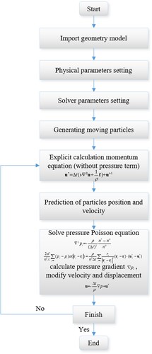
3.6. Numerical scheme for the flow analysis

The momentum equation is solved by a semi-implicit method. In the first step, the effects of viscous force and body force are considered. Then the pressure equation is solved by using the velocity field. Finally, the velocity is corrected by calculating the pressure gradient. The most important aspect in the calculation method is that the pressure field is estimated based on the Poisson equation. The criterion of the end of calculation is to check whether the end time of calculation has been completed and, if not, go to the next time step to calculate. The process of numerical calculation is shown in Figure 2. The inlet boundary condition is the flow rate, and the outlet boundary condition is atmospheric pressure. As the oil entering the bearing cavity is stirred by the high-speed rotating bearing inner ring, roller and cage, the turbulence model is selected. To improve simulations where turbulence plays an important role, the widely used model is implemented into the method (Smagorinsky, 1963). It is a zero equation turbulence model. The turbulent viscosity coefficient formula is as follows: (10) ${\mu }_t=\text{(}{C}_s\mathrm{\Delta }X{\text{)}}^{\text{2}}|\overline{S}|$(10) $\mathrm{\Delta }X$ is the particle space, $C_s$ is the Smagorinsky constant, and $\overline{S}$ is the mean strain rate.

Figure 2. The flow chart of numerical solution.

The heat transfer model isn’t considered in the calculation process. Considering the viscous term in the momentum equation, the time step needs to meet the Morris condition(Liu & Liu, 2003). The time step is 0.0001 s according to the following formula. (11) $\mathrm{\Delta }t\le 0.125\frac{h^{\text{2}}}{\nu }$(11) h is effective radius.

Generally, the particle radius has a certain influence on the calculation results. In order to ensure that there can be three layers of particles between the cage and the inner or outer ring, the particle radius of 0.35, 0.4 and 0.5 mm are used to verify the independence of particle radius. When the rotating speed of bearing is 600 r/min, the results of churning torque of balls and cage under different particle radius are shown in Table 3. The difference of churning torque between particle radius of 0.4 and 0.35 mm is less than 10%, considering the economy of calculation. In all the following calculations, the particle radius is 0.4 mm.

Table 3 Results of churning torque of balls and cage under different particle radius.

Particle radius(mm)	Total number of particles	Torque(mN·m)
0.35	355203	3.01
0.4	265083	3.28
0.5	131966	4.80

The momentum equation can be discretized into: (12) $\frac{\mathbf{\text{u}}\text{ - }{\mathbf{\text{u}}}^{t-1}}{\Delta t}=-\frac{1}{\rho }\mathrm{\nabla }p\text{ + }\nu {\mathrm{\nabla }}^{\text{2}}\mathbf{\text{u}}\text{ + }\frac{1}{\rho }\mathbf{\text{f}}$(12) where Equation (12) can be written as the following equation (13) $\mathbf{\text{u}}=-\frac{\Delta t}{\rho }\mathrm{\nabla }p\text{ + }\Delta t\text{(}\nu {\mathrm{\nabla }}^{\text{2}}\mathbf{\text{u}}\text{ + }\frac{1}{\rho }\mathbf{\text{f}}\text{) + }{\mathbf{\text{u}}}^{t-1}$(13) where predicted velocity u* is (14) ${\mathbf{\text{u}}}^{\ast }=\Delta t\text{(}\nu {\mathrm{\nabla }}^{\text{2}}\mathbf{\text{u}}\text{ + }\frac{1}{\rho }\mathbf{\text{f}}\text{) + }{\mathbf{\text{u}}}^{t-1}$(14) And Equation (14) can be formulated as: (15) $\mathbf{\text{u}}=-\frac{\mathrm{\Delta }t}{\rho }\mathrm{\nabla }p+{\mathbf{\text{u}}}^{\ast }$(15) Equation (15) can be formulated as: (16) $\mathrm{\nabla }\cdot \mathbf{\text{u}}=-\frac{\mathrm{\Delta }t}{\rho }\mathrm{\nabla }\cdot \mathrm{\nabla }p+\mathrm{\nabla }\cdot {\mathbf{\text{u}}}^{\ast }$(16) Apparently, the left side of the equation is 0. The equation is transformed into (17) ${\mathrm{\nabla }}^{2}p=\frac{\rho }{\Delta t}\mathrm{\nabla }\cdot {\mathbf{\text{u}}}^{\ast }$(17) The original Poisson Pressure Equation proposed by Koshizuka and Oka (1996) is (18) ${\mathrm{\nabla }}^2{p}_i=-\frac{\rho }{{(\Delta t)}^2}\frac{n^{\ast }-n^0}{n^0}$(18) The following modified Poisson Pressure Equation was proposed by Khayyer and Gotoh (2009). (19) ${\mathrm{\nabla }}^2{p}_i=\frac{\rho }{n^0\Delta t}\sum _{j\ne i}\frac{r_e}{{|{\mathbf{\text{r}}}_j-{\mathbf{\text{r}}}_i|}^3}({\mathbf{\text{r}}}_j-{\mathbf{\text{r}}}_i)\cdot ({\mathbf{\text{u}}}_j^{\ast }-{\mathbf{\text{u}}}_i^{\ast })$(19) According to the Poisson Pressure Equation of Equation (8), we can get the following equations: (20) $\begin{array}{rl}& \frac{2d}{n^0\lambda }\sum _{j\ne i}(p_j-p_i)\omega (|{\mathbf{\text{r}}}_j-{\mathbf{\text{r}}}_i|)\\ & =\frac{\rho }{n^0\Delta t}\sum _{j\ne i}\frac{r_e}{{|{\mathbf{\text{r}}}_j-{\mathbf{\text{r}}}_i|}^3}({\mathbf{\text{r}}}_j-{\mathbf{\text{r}}}_i)\cdot ({\mathbf{\text{u}}}_j^{\ast }-{\mathbf{\text{u}}}_i^{\ast })\end{array}$(20)

3.7. Boundary condition

3.7.1. Free surface boundary condition

Boundary conditions are essential for solving the Poisson pressure equation. Commonly, the ambient pressure is the boundary condition of the free surface. Shibata et al. (2015) proposed the concept of virtual particles. The calculation formula of virtual particles is as follows: (21) $n_{i,\text{virtual}}=max(n^0-n_i,0)$(21) Then the Poisson equation is (22) $\begin{array}{rl}& \frac{2d}{n^0\lambda }\left[\sum _{j\ne i}(p_j-p_i)\omega (|{\mathbf{\text{r}}}_j-{\mathbf{\text{r}}}_i|)+(p_{\text{virtual}}-p_i)n_{i,\text{virtual}}\right]\\ & =\frac{\rho }{n^0\Delta t}\sum _{j\ne i}\frac{r_e}{{|{\mathbf{\text{r}}}_j-{\mathbf{\text{r}}}_i|}^3}({\mathbf{\text{r}}}_j-{\mathbf{\text{r}}}_i)\cdot ({\mathbf{\text{u}}}_j^{\ast }-{\mathbf{\text{u}}}_i^{\ast })\end{array}$(22)

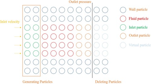
3.7.2. Inlet and outlet boundary

For the inlet boundary, the new particles with a given velocity are generated over time. The inlet particles are involved in the numerical density calculation, but not in the pressure calculation. Before the inlet particles cross the inlet border, they play as ‘inlet particles’ with an inlet velocity. When the inlet particles exceed the inlet border, they are transformed into actual fluid particles automatically.

For the outlet boundary, the outlet pressure is given to the virtual particles outside the border. The fluid particles are deleted, when they exceed the outlet border. The particle diagram of the inlet and outlet boundary is shown in Figure 3.

Figure 3. Inlet and outlet boundary.

4. Experimental apparatus

To obtain the oil distribution of bearing lubrication at different speeds, single lens reflex (SLR) camera and other equipment are used to capture clear pictures to analyze the distribution of lubricating oil. The test rig is mainly comprised of the motorized spindle, SLR camera, temperature sensor, motor controller, parallel light, test bearing and a peristaltic pump, as shown in Figure 4. The motor controller can control the speed of the motor, thus controlling the speed inner ring. The peristaltic pump is composed of gear pump and brushless DC motor, which can regulate the flow rate of the oil supply. The specific parameters of the test apparatus and sensor are shown in Table 4. When taking pictures with SLR camera, in order to obtain a clear picture of the distribution of lubricating oil in the bearing cavity, it is necessary to select an appropriate shutter speed according to the rotating speed of the bearing. The selection basis of shutter speed is shown in Table 5. During the test, first irradiate the parallel light on the bearing end face, then select the appropriate shutter speed, set the appropriate aperture, and finally take photos.

Figure 4. Visual experimental device for bearing lubrication flow field (a) Physical experimental device diagram (b) Schematic diagram of the experimental device.

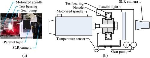
Table 4 Technical parameters of equipment.

Description	Detail
Motorized spindle	GDZ120 × 103-6, range 0–18000 r/min
Motor controller	B3000-4T0055G/0075P, accuracy±0.5%
Peristaltic pump	LabGV, range 80∼2400 ml/min, accuracy ±1%
Temperature sensor	Range −70∼500°C, accuracy ±0.2%
Camera lens	ASPHERICAL LD XR Di II, AF 17–50 F/2.8

Table 5 The selection basis of shutter speed.

Bearing rotation speed	Shutter speed
<1000 r/min	1/500 s
1000 r/min∼2000 r/min	1/1000 s
2000 r/min∼5000 r/min	1/2000 s
>5000 r/min	1/4000 s

5. Results and discussion

5.1. Distribution of lubricating oil

Numerical simulation and visualization experiments are used to study the internal flow field of oil-jet lubrication bearings at speeds of 600, 1200, 2400, 4800, 6000, 9000, 10000 and 12000 r/min. The nozzle radius is 0.5 mm. The flow rate of the oil supply is 500 mL/min. The injection speed of lubricating oil is about 10.6 m/s, which can meet the demand of injection speed.

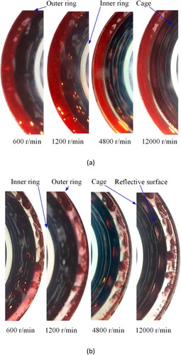
As shown in Figure 5, visualization test results of the flow field at different speeds are presented. Most of the oil is ejected from the gap between the rolling element and the inner and outer raceways, and between the rolling element and the cage when the bearing is stationary. The cage, rolling element and the end face of inner and outer rings can be clearly seen, because the whole bearing cavity is not filled with oil. When the rotation speed is less than 1200 r/min, the bearing cavity is covered with a thick lubricating oil layer. When the rotational speed is greater than 2400 r/min, the oil layer attached to the bearing cavity becomes thinner. With the increase of speed, the contour of the ball and cage becomes more and more evident. Therefore, it can be known that the oil content decreases with the increase of rotating speed. It is because that the oil tends to be thrown centrifugally with a higher rotation speed from the bearing cavity. The storage time of the oil becomes shorter.

Figure 5. Visualization test results of the flow field at different speeds.

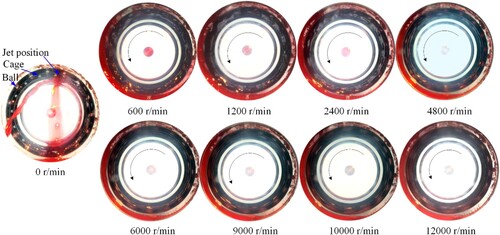
When the speed is 4800 r/min, the profile of the cage and balls in the bearing cavity is becoming more and more apparent along the circumferential direction, and there is less oil attached to the surface. There is relatively a smaller amount oil of upstream position of the oil outlet, which is consistent with the calculated results (Hu et al., 2014). In addition, the oil passing through the bearing cavity mainly leaves the bearing from the downstream direction of the nozzle. From the nozzle position along the bearing rotation direction of 120°, the end face oil layer of the bearing outer ring is relatively thick. Following along the direction of rotation, the oil layer on the outer ring face begins to decrease and shrink until the bottom of the outer end face of the bearing.

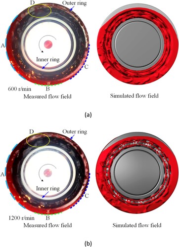
As shown in Figure 6, the measured and calculated visual flow field results are displayed at speeds of 600 and 1200 r/min. When the speed is 600 r/min, a large amount of oil is observed in the bearing cavity. The clearance between cage and balls, between balls and inner ring, and between balls and outer ring are covered by a thick oil layer, making it difficult to distinguish the boundary between bearing cage and balls. The oil content in the A region of the end face is relatively high. The oil is first thrown into this region by centrifugal force. Mainly due to gravity, part of the oil in the A and C regions is collected in the B region. There is less oil in the C region, because it is far from the jet position. It can be seen in the D region that the oil directly flies away from the bearing, which is closely related to the jet position. When the speed is 1200 r/min, it has a similar effect. The numerical calculation results agree with the experimental results. The reason for the difference between the numerical calculation results and the measured results may be that the effect of air on the fluid is not considered in the numerical calculation.

Figure 6. The measured and calculated results of the visual flow field at different speeds (a) The speed is 600 r/min. (b) The speed is 1200 r/min.

As shown in Figure 7, the measured and calculated results of the visual flow field are displayed at speeds of 4800 r/min and 12000 r/min. As the rotation speed increases, the centrifugal force acting on the oil entering the bearing cavity becomes stronger and stronger. Therefore, the oil is thrown out, leaving less oil in the bearing cavity attached to the cage and ball surface. Ball surface and the contour of cage and ball become more and more apparent. The difference between the test results and the simulation results may be due to the effect of air on the fluid, cage and ball when the bearing is at high speed during the test. The impact of air on the bearing lubrication flow field is not considered in the simulation computation. In addition, during the experiment, the oil temperature will change to a certain extent. It is assumed that the oil temperature is constant in the numerical calculation, which may also be the reason for the difference.

Figure 7. The measured and calculated results of the visual flow field at different speeds (a) The speed is 4800 r/min. (b) The speed is 12000 r/min.

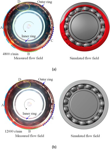
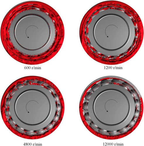
Figure 8 shows the numerical calculation results of the flow field at the outlet side. It is similar to the flow field changes with the other side at different speeds. As the rotation speed increases, the oil layer in the bearing cavity becomes thinner, and the contour of the cage and ball gradually becomes clear. In addition, more broken oil droplets can be seen in the bearing cavity. Therefore, at high-speed, it is difficult to form a complete oil film inside the bearing cavity.

Figure 8. The simulated flow field in the side of the oil outlet.

As shown in Figure 9, the enlarged visualization flow field of the test results at different speeds is presented. It shows the evolution process of the bearing cavity internal flow field on both sides of the jet position at different rotating speeds. It can be observed from the enlarged picture that the oil layer in the bearing cavity downstream of the jet position is slightly higher than that in the upstream. In addition, some lubrication oil penetrates the bearing cavity. The remaining oil flows into the bearing cavity and will move with the balls and cage. Due to the small inertia of the oil, it will accelerate rapidly to the same speed as the cage and the inner ring. It is thrown out of the bearing cavity and leaves from the bearing cavity downstream of the jet position. As the rotation speed increases, the region away from the bearing shrinks towards the jet position. When the rotation speed is 12000 r/min, under the irradiation of parallel light source, the surface of the bearing ball has an evidently reflective surface, which indicates that the oil layer thickness is relatively thin.

Figure 9. Enlarged visualization of the flow field of test results at different rotation speeds (a) The left side of the bearing. (b) The right side of the bearing.

5.2. Particle number distribution and churning torque

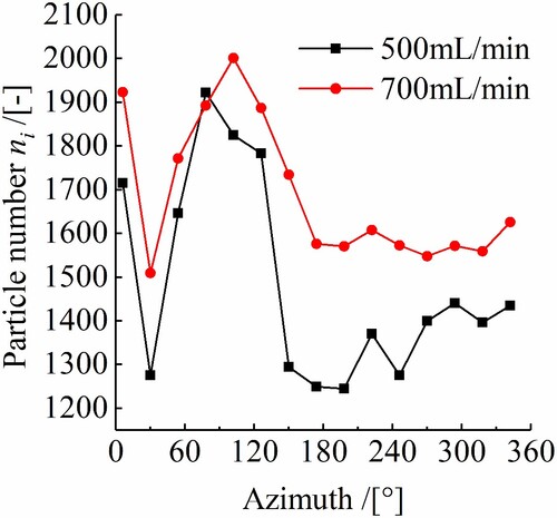
To quantitatively analyze the oil content, a cuboid zone is established in the bearing cavity to count the number of particles in each region. When the oil flow rate is 500 mL/min, the rotation speed is 600 and 1200 r/min, and the nozzle diameter is 1 mm, the distribution of the number of particles in the bearing cavity along the rotation direction is shown in Figure 10. The number of particles decreases from the nozzle position to about 30° along the direction of rotation, then increases from about 30° to 110°, and finally decreases from about 110° to the nozzle position. The number of particles is relatively large between about 90° and 120°, which means that there is more oil in the bearing cavity. It is consistent with the result in Figure 6. As the rotation speed increases, the number of particles in the corresponding position along the rotation direction becomes smaller. When the oil flow rate is 500 and 700 mL/min, the injection speed is constant, and the rotation speed is 1200 r/min, the distribution of particle number along the rotation direction is shown in Figure 11. As the increase of flow rate, the number of particle in the corresponding position along the rotation direction increases. The behavior of particle number along the rotation direction is the same.

Figure 10. Particle number distribution at different speeds.

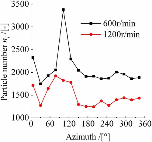
Figure 11. Particle number distribution with the oil flow rate of 500 and 700 mL/min.

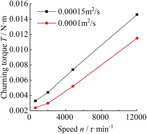
When the flow rate of oil supply is 500 mL/min, the nozzle radium is 0.5 mm, and the kinetic viscosity is 0.00015 m²/s and 0.0001 m²/s, the variation of oil churning torque of bearing cage and ball with rotating speed is presented in Figure 12. The churning torque of ball and cage increases linearly with the increase of rotating speed. Peterson et al. (2021) obtained that the drag force increases with the increase of rotation speed. There is the same trend with the results of the study. In addition, at the same speed, the churning torque increases with the increase of kinetic viscosity.

Figure 12. Variation of the churning torque of balls and cage with rotating speed.

6. Conclusions and future work

The MPS numerical method is applied to the visualization of ball bearings lubrication flow field. The numerical results are verified by visualization experiments. The oil distribution in bearing cavity under different speeds is discussed. The variation of churning torque between roller and cage at different speeds, flow rates and viscosity are studied. The conclusion is as follows:

1. The oil distribution along the rotation direction obtained by MPS numerical calculation method has the same trend as the experimental results. It is uneven with the distribution of oil in the bearing cavity

2. Along the rotation direction, the number of particles first decreases, then increases and finally decreases. The number of particles is relatively large between about 90°and 120°.

3. As the increase of speed, the number of particles in the bearing cavity decreases. As the increase of flow rate, the number of particles in the bearing cavity increases.

4. The churning torque of the bearing cage and balls changes linearly with the increase of rotation speed. At the same speed, as the decrease of kinematic viscosity, the churning torque of the ball and cage decreases.

Finally, it is worth mentioning that the air has a significant impact on the oil distribution at high speed. Next, the oil-air two-phase flow will be added to the numerical model and we will compare and analyze with Peterson et al. (2021). That will be of significant benefit to the design of ball bearings.

Disclosure statement

No potential conflict of interest was reported by the author(s).

Additional information

Funding

This work was supported by National Natural Science Foundation of China [grant number 51975045].

References

- Adeniyi, A. A., Morvan, H., & Simmons, K. (2017). A computational fluid dynamics simulation of oil-air flow between the cage and inner race of an aero-engine bearing. Journal of Engineering for Gas Turbines and Power-Transactions of the ASME, 139(1). Article 012506. https://doi.org/10.1115/1.4034210
- Aidarinis, J., Missirlis, D., Yakinthos, K., & Goulas, A. (2011). CFD modeling and LDA measurements for the air-flow in an aero engine front bearing chamber. Journal of Engineering for Gas Turbines and Power-Transactions of the ASME, 133(8). Article 082504. https://doi.org/10.1115/1.4002830
- Bossmanns, B., & Tu, J. F. (1999). A thermal model for high speed motorized spindles. International Journal of Machine Tools & Manufacture, 39(9), 1345–1366. https://doi.org/10.1016/s0890-6955(99)00005-x
- Bristot, A., Morvan, H. P., & Simmons, K. A. (2016). Evaluation of a volume of fluid CFD methodology for the oil film thickness estimation in an aero-engine bearing chamber. Volume 2C: Turbomachinery, https://doi.org/10.1115/gt2016-56237
- Chang, Z., Jia, Q., Yuan, X., & Chen, Y. L. (2017). Main failure mode of oil-air lubricated rolling bearing installed in high speed machining. Tribology International, 112, 68–74. https://doi.org/10.1016/j.triboint.2017.03.024
- Chen, R. H., Dong, C. H., Guo, K. L., Tian, W. X., Qiu, S. Z., & Su, G. H. (2020). Curr-ent achievements on bubble dynamics analysis using MPS method. Progress in Nuclear Energy, 118. Article 103057. https://doi.org/10.1016/j.pnucene.2019.103057
- Crouchez-Pillot, A., & Morvan, H. (2014, June 16–20). CFD simulation of an aeroengine bearing chamber using an enhanced volume of fluid (VOF) method: An evaluation using adaptive meshing. Proceedings of ASME Turbo Expo 2014: Turbine Technical Conference and Exposition. Düsseldorf, Germany.
- Duan, G. T., Chen, B., Zhang, X. M., & Wang, Y. C. (2017). A multiphase MPS solver for modeling multi-fluid interaction with free surface and its application in oil spill. Computer Methods in Applied Mechanics and Engineering, 320, 133–161. https://doi.org/10.1016/j.cma.2017.03.014
- Duan, G. T., Koshizuka, S., Yamaji, A., Chen, B., Li, X., & Tamai, T. (2018). An accurate and stable multiphase moving particle semi-implicit method based on a corrective matrix for all particle interaction models. International Journal for Numerical Methods in Engineering, 115(10), 1287–1314. https://doi.org/10.1002/nme.5844
- Fondelli, T., Andreini, A., Da Soghe, R., Facchini, B., & Cipolla, L. (2015, June 15–19). Volume of fluid (VOF) analysis of oil-jet lubrication for high-speed spur gears using an adaptive meshing approach. Proceedings of ASME Turbo Expo 2014: Turbine Technical Conference and Exposition. Montréal, Canada.
- Gao, W. J., Lyu, Y. G., Liu, Z. X., & Nelias, D. (2019). Validation and application of a numerical approach for the estimation of drag and churning losses in high speed roller bearings. Applied Thermal Engineering, 153, 390–397. https://doi.org/10.1016/j.applthermaleng.2019.03.028
- Gao, W. J., Nelias, D., Li, K., Liu, Z. X., & Lyu, Y. G. (2019). A multiphase computati-onal study of oil distribution inside roller bearings with under-race lubrication. Tribology International, 140. Article Unsp 105862. https://doi.org/10.1016/j.triboint.2019.105862
- Gao, W. J., Nelias, D., Lyu, Y. G., & Boisson, N. (2018). Numerical investigations on drag coefficient of circular cylinder with two free ends in roller bearings. Tribol-ogy International, 123, 43–49. https://doi.org/10.1016/j.triboint.2018.02.044
- Ghalandari, M., Bornassi, S., Shamshirband, S., Mosavi, A., & Chau, K. W. (2019). Investigation of submerged structures’ flexibility on sloshing frequency using a boundary element method and finite element analysis. Engineering Applications of Computational Fluid Mechanics, 13(1), 519–528. https://doi.org/10.1080/19942060.2019.1619197
- Gloeckner, P. (2013). The influence of the raceway curvature ratio on power loss and temperature of a high speed jet engine ball bearing. Tribology Transactions, 56(1), 27–32. https://doi.org/10.1080/10402004.2012.725123
- Gorse, P., Busam, S., & Dullenkopf, K. (2006). Influence of operating condition and geometry on the oil film thickness in aeroengine bearing chambers. Journal of Engineering for Gas Turbines and Power-Transactions of the ASME, 128(1), 103–110. https://doi.org/10.1115/1.1924485
- Gotoh, H., & Khayyer, A. (2018). On the state-of-the-art of particle methods for coastal and ocean engineering. Coastal Engineering Journal, 60(1), 79–103. https://doi.org/10.1080/21664250.2018.1436243
- Guo, D., Chen, F. C., Liu, J., Wang, Y. W., & Wang, X. (2020). Numerical modeling of churning power loss of gear system based on moving particle method. Tribo-logy Transactions, 63(1), 182–193. https://doi.org/10.1080/10402004.2019.1682212
- Harris, T. A., & Kotzalas, M. N. (2006). Advanced concepts of bearing technology: Rolling bearing analysis (5th ed.). Taylor & Francis Press.
- Hu, J. B., Wu, W., Wu, M. X., & Yuan, S. H. (2014). Numerical investigation of the air-oil two-phase flow inside an oil-jet lubricated ball bearing. International Journal of Heat and Mass Transfer, 68, 85–93. https://doi.org/10.1016/j.ijheatmasstransfer.2013.09.013
- Khayyer, A., & Gotoh, H. (2009). Modified moving particle semi-implicit methods for the prediction of 2D wave impact pressure. Coastal Engineering, 56(4), 419–440. https://doi.org/10.1016/j.coastaleng.2008.10.004
- Koshizuka, S., & Oka, Y. (1996). Moving-particle semi-implicit method for fragmentation of incompressible fluid. Nuclear Science and Engineering, 123(3), 421–434. https://doi.org/10.13182/nse96-a24205
- Koshizuka, S., Tamako, H., & Ya, O. (1995). A particle method for incompressible viscous flow with fluid fragmentation. Comput. Journal of Computational Fluid Dynamics, 4(1), 29–46.
- Lee, C. W., Palma, P. C., Simmons, K., & Pickering S. J. (2005). Comparison of computational fluid dynamics and particle image velocimetry data for the airflow in an aeroengine bearing chamber. Journal of Engineering for Gas Turbines and Power, 127(4), 697–703. https://doi.org/10.1115/1.1924635
- Liu, G. R., & Liu, M. B. (2003). Smoothed particle hydrodynamics: A meshfree particle method. World Scientific.
- Nagaoka, T., Takemoto, M., & Ogasawara, S. (2015, October 25–28). Rotor design of a 150 kW 6,000 rpm/25,000 rpm high speed induction motor for testing equipment of EV/HEV traction motors. 2015 18th International conference on Electrical Machines and Systems (ICEMS). Pattaya City, Thailand.
- Noda, T., Shibasaki, K., Miyata, S., & Taniguchi, M. (2016). X-ray ct imaging of grease behavior in ball bearing and numerical validation of multi-phase flows simulation. Tribology Online, 61(4), 275–284. https://doi.org/10.2474/trol.15.36
- Pang, B. T., Li, J. S., Liu, H. B., Ma, W., & Xue, Y. J. (2008). A simulation study on optimal oil spraying mode for high-speed rolling bearing. Journal of Achievement in Materials and Manufacturing Engineering, 31(2), 553–557.
- Peterson, W., Russell, T., Sadeghi, F., Berhan, M. T., Stacke, L. E., & Ståhl, J. (2021). A CFD investigation of lubricant flow in deep groove ball bearings. Tribology International, 154, 106735. https://doi.org/10.1016/j.triboint.2020.106735
- Salih, S. Q., Aldlemy, M. S., Rasani, M. R., Ariffin, A. K., Ya, T. M. Y. S. T., Nadhir, A. A., Yaseen, Z. M., Chau, K. W., & Al-Ansari N. (2019). Thin and sharp edges bodies-fluid interaction simulation using cut-cell immersed boundary method. Engineering Applications of Computational Fluid Mechanics, 13(1), 860–877. https://doi.org/10.1080/19942060.2019.1652209
- Shibata, K., Masaie, I., Kondo, M., Murotani, K., & Koshizuka, S. (2015). Improved pressure calculation for the moving particle semi-implicit method. Computational Particle Mechanics, 2(1), 91–108. https://doi.org/10.1007/s40571-015-0039-6
- Smagorinsky, J. (1963). General circulation experiments with the primitive equations: I. The basic experiment. Monthly Weather Review, 91(3), 99–164. https://doi.org/10.1175/1520-0493(1963)091<0099:GCEWTP>2.3.CO;2
- Sun, Z. G., Chen, X., Xi, G., Liu, L., & Chen, X. (2017). Mass transfer mechanisms of rotary atomization: A numerical study using the moving particle semi-implicit method. International Journal of Heat and Mass Transfer, 105, 90–101. https://doi.org/10.1016/j.ijheatmasstransfer.2016.09.053
- Wu, W., Hu, C. H., Hu, J. B., & Yuan, S. H. (2016). Jet cooling for rolling bearings: Flow visualization and temperature distribution. Applied Thermal Engineering, 105, 217–224. https://doi.org/10.1016/j.applthermaleng.2016.05.147
- Wu, W., Hu, C. H., Hu, J. B., Yuan, S. H., & Zhang, R. (2017). Jet cooling characteristics for ball bearings using the VOF multiphase model. International Journal of Thermal Sciences, 116, 150–158. https://doi.org/10.1016/j.ijthermalsci.2017.02.014
- Wu, W., Hu, J. B., Yuan, S. H., & Hu, C. H. (2016b). Numerical and experimental investigation of the stratified air-oil flow inside ball bearings. International Journal of Heat and Mass Transfer, 103, 619–626. https://doi.org/10.1016/j.ijheatmasstransfer.2016.07.090
- Yan, K., Dong, L., Zheng, J. H., Li, B. T., Wang, D. F., & Sun, Y. J. (2018). Flow performance analysis of different air supply methods for high speed and low friction ball bearing. Tribology International, 121, 94–107. https://doi.org/10.1016/j.triboint.2018.01.035