Hydrodynamic behaviors of self-propelled sperms in confined spaces

ABSTRACT

The hydrodynamic behaviors of sperms in confined spaces (e.g. Poiseuille flow and quiescent flow between two parallel walls) are studied with a two-dimensional self-propelled sperm model based on the immersed boundary-lattice Boltzmann method (IB-LBM). For single-sperm swimming in Poiseuille flow, four typical swimming patterns, including wall-adhesion, focusing, tumbling and oscillating, are observed. The occurrence conditions including flow strength, inter-wall distance, initialization of sperm are studied in detail for the four patterns. For multiple-sperm swimming in quiescent flow between two parallel walls, it is observed that the sperm population tends to swim nearby the walls, leading to wall accumulation. To explore the hydrodynamic behaviors of the sperm population in Poiseuille flows, the effects of flow velocities on the sperm rheotaxis and the wall accumulation are investigated in detail. It is found that an appropriate flow velocity is essential to guide the swimming direction, as well as the wall accumulation. In addition, collision and adsorption between adjacent sperms may facilitate wall accumulation. Finally, we study the propulsion rate of different combination modes of sperms. We found that the wedge-shaped mode leads to the optimal propulsive speed, and reducing the combining distance can increase the propulsive speed.

KEYWORDS:

• Sperm population
• self-propelled
• Poiseuille flow
• IB-LBM
• sperm rheotaxis
• wall accumulation

1. Introduction

Understanding sperm swimming behaviors has important practical significance in many aspects. For example, the motility of sperm cells is closely related to the reproductive function of animals. The complex biochemical and hydrodynamic mechanisms of sperm swimming have attracted substantial attention in the past few years (Campuzano et al., 2017; Ishimoto & Gaffney, 2015; Magdanz et al., 2017; Xu et al., 2017). Due to the increasing infertility rate, reproductive medicine and the more effective sperm selection techniques in vitro have been developed rapidly in recent years (Seandel & Rafii, 2011; Thapa & Heo, 2019), which bring hope to people with reproductive defects. In addition, the swimming mechanisms of sperms can well inspire the development of nano/micro-robots (Magdanz et al., 2017), making the targeted drug delivery possible (Campuzano et al., 2017; Xu et al., 2018).

Due to its importance, great effort has been made to study the behaviors of sperm swimming (Tian & Wang, 2021). Recent studies on the mechanisms of sperm swimming have shown that some biological, chemical and physical factors may affect the direction of sperm swimming. These factors include the direction of fluid flow (Ishimoto & Gaffney, 2015; Omori & Ishikawa, 2016; Zhang et al., 2016), the temperature (Bahat et al., 2012; Boryshpolets et al., 2015), the concentration of some chemical substances (Ramírez-Gómez et al., 2020; Strunker et al., 2011), the effect of wall boundary (Elgeti et al., 2010; Ishimoto et al., 2016; Ishimoto & Gaffney, 2014; Liu et al., 2020; Nosrati et al., 2015; Smith et al., 2009) and the interaction between sperms (Fisher et al., 2014; Ishimoto & Gaffney, 2018) etc. They provide clues on the sperm's journey to the egg. Studies have shown that sperms swimming synchronously and closely could adsorb each other and swim together as a cluster (Nosrati et al., 2015; Woolley et al., 2009; Yang et al., 2008). However, the significance of such phenomenon for sperm migration still requires further study, especially for human sperms. As a sperm swims in a confined space, it tends to adhere and gather to the wall, which is recognized as wall accumulation of sperm and has been studied (Denissenko et al., 2012; Nosrati et al., 2015; Smith et al., 2009), partially revealing the associated flow physics. These studies have reported the diversity of sperm behaviors near the wall and mechanisms for cell gathering. In addition, previous works mainly explain the rheotaxis of sperms as a completely passive phenomenon, which is primarily determined by the shear flow near the wall (Schiffer et al., 2020; Zhang et al., 2016). However, the swimming mechanism of sperms near the wall is very complex, and needs to be further studied, especially on exploring other factors that may affect the occurrence of rheotaxis.

With the rapid development of computer and numerical simulation technologies, some important numerical models have been proposed to study the hydrodynamic mechanisms associated with sperm swimming. Since sperm swimming is under the condition of low Reynolds number, such flow is generally simulated by solving the Stokes equation with the finite difference method, finite volume method, finite element method, spectral method or the most commonly used boundary element method (Ishimoto & Gaffney, 2017; Tian & Wang, 2021). In addition, multi-particle collision dynamics was applied by Elgeti et al. to simulate such low Reynolds number flow, and combined with the resistive force theory to study the sperm swimming near the wall (Elgeti et al., 2010). A ‘node-spring’ structure is generally adopted to model the sperm. Therein the swing of the sperm tail is generated by the movement of the preset nodes, and coupled with fluid flow. Different methods, such as the resistive force theory (Friedrich et al., 2010; Hyakutake et al., 2019), Stokeslet Equation (Cortez et al., 2005) and immersed boundary method (Dillon & Zhuo, 2010; Peskin, 2003; Salih et al., 2019) are used to exchange the information between the flow and the structure. Although these models promote understanding of sperm swimming, there are some limitations. Firstly, the mass sperm simulation generally requires large-scale computing, and consequently results in low computational efficiency. Secondly, for multiple sperm swimming, dealing with the interactions between the moving sperms is quite a challenge. Therefore, it is necessary to develop a more feasible model to study swarm behaviors of sperms.

Multiple sperms swimming in a confined space involve sperm-sperm and sperm-wall interactions, leading to complicated behaviors in the migration of sperms. To further understand the sperm behaviors, it is necessary to study the performances (such as the evolutions of swimming direction and spatial distribution of sperms) of the sperm population in confined flows. In addition, the mechanisms associated with complicated sperm behaviors are not fully understood. Specifically, it is unclear whether the rheotaxis and wall accumulation are merely determined by the hydrodynamic factors and how the collision and adsorption between sperms affect swimming efficiency. These issues will be addressed by an improved 2D sperm swimming model coupled with the IB-LBM (Tian et al., 2013; Xu et al., 2017), which is based on our previous studies (Liu et al., 2020; Xu et al., 2018). In (Xu et al., 2018), we showed that the wall in a viscous fluid could capture a piece of vibrating filament nearby it, which implies an effect of ‘wall attraction’. Corresponding analysis indicated that such effect is mainly induced by the asymmetrical pressure distribution on both sides of the filament. This study provided a theoretical explanation for why sperms tend to swim near a solid surface. In the present study, we discuss a swimming pattern named wall-adhesion, which is essentially a ‘wall attraction’ phenomenon. In addition, in (Liu et al., 2020), we proposed two types of swimming sperm models using IB-LBM and mainly discussed the reason for ‘wall acceleration’, for which the sperm can only swim along a fixed line. In this paper, we improved the model to free-swimming, introduced the sperm population, and focused on the swimming patterns and distribution principles during sperm motion.

This paper proposed a self-propelled sperm using IB-LBM, which can swim freely in the flow field. This model is relatively simple, driven with explicit force, and easily implemented by parallel computing. These advantages make it suitable to deal with quantitative analysis of sperm swimming and to model multi-sperms. Particularly, sperm swimming in a confined space (i.e. the actual scene of a microchannel (Denissenko et al., 2012) (Ghalandari et al., 2019)) was studied. And three main aspects were discussed emphatically. The first aspect is for single sperm swimming in a Poiseuille flow, where four swimming patterns, including wall-adhesion, focusing, tumbling, and oscillating, were exhibited and analyzed. The second aspect is for sperm population swimming in quiescent and Poiseuille flow, which mainly focuses on the effects of flow velocities on the sperm rheotaxis and the wall accumulation. The third one is to study the propulsion rate of different combination modes of sperms. We hope that these studies can improve our understanding of the hydrodynamic behavior of human sperm and result to development of in vitro sperm optimization technology.

The rest of this paper is organized as follows. The mathematical formulation is outlined in Section 2. Section 3 presents the results. The conclusions are provided in Section 4.

2. Model and numerical details

2.1. Physical model

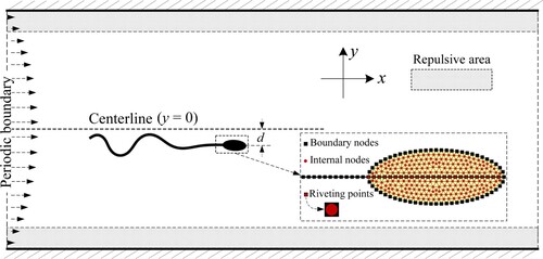
On the journey to the egg cell, the sperm experiences a complex flow environment, including the uneven surfaces of reproductive cavities, narrow folds and channels, etc. For the wall accumulation phenomenon of sperm cells, their behaviors are closely related to the surface of the boundary in the flow field. To study the influence of the boundary and the shear flow on sperm swimming, we developed a model of sperm swimming in the Poiseuille flow between two parallel walls, as shown in Figure 1.

Figure 1. Schematic diagram of sperm swimming in a confined space.

Typically, the length of mammalian (human) sperm is between $50\sim 60\text{μ}\mathrm{m}$ in nature (Elgeti et al., 2015; Ishimoto & Gaffney, 2014; Nosrati et al., 2015). Thus the body length ${\text{L}}_s$ of sperm cells is set as $55\text{μ}\mathrm{m}$ in the model. The sperm tail is composed of 221 equidistant nodes, with $L_s=220\mathrm{\Delta }s$. $\mathrm{\Delta }s$ is the node spacing and is set to be equidistant from the background (fluid) grid, so $\mathrm{\Delta }s=\mathrm{\Delta }x=\mathrm{\Delta }y=0.25\text{μ}\mathrm{m}$. The swing frequency of the tail in the model is set to 15 Hz (Gadêlha et al., 2020) (Wagenaar et al., 2016), and its dynamic shape refers to Ref. (Kantsler et al., 2014). Therefore, the swing period of the tail is $T=\frac{1}{15}s$, which includes $6000\mathrm{\Delta }t$ in our simulations.

In this paper, the flow field is computed in a rectangular domain, which is $300\text{μ}\mathrm{m}$ in length and $200\text{μ}\mathrm{m}$ in width, or expressed by $L_{\text{c}}\times W_{\text{c}}=5.45{\text{L}}_{\text{s}}\times 3.36{\text{L}}_{\text{s}}$ measured by the body length of sperm. This size is default unless otherwise stated. The upper and lower sides of the flow field are solid non-slip walls, and the left and right sides are periodic boundaries. Because the disturbance of sperm on fluid happens merely in a limited range around itself, the setting of computational domain size is large enough to avoid the unphysical effects from the periodic flow. The inter-wall distance $W_{\text{c}}$ can be adjusted as required. The fluid density is $\rho =1\text{g}/\text{ml}$, and the dynamic viscosity is $\mu =0.001\text{Pa}\cdot \text{s}$ (referring to water at room temperature). An external force $f_{\text{d}}$ parallel to the wall is applied to drive the flow. $f_{\text{d}}=0$ means the fluid is static, and $f_{\text{d}}\ne 0$ means producing a Poiseuille flow. The relationship between $f_d$ and the maximum flow velocity $U_{max}$ of Poiseuille flow is (Sun et al., 2013): (1) $U_{max}=\rho f_{\text{d}}{W}_{\text{c}}^2/\left(8\mu \right).$(1) In our simulations, sperms are set to freely cross the periodic boundaries, so that this model allows sperm to swim in an infinite region along the walls. In Figure 1, $d$ is the distance from the front vertex of the head to the midline between the walls. When above the midline, $d>0$, and when below the midline, $d<0$. As the sperm is close to a wall, the tail swing perpendicularly to the solid surface will be restricted, leading to the loss of propulsive force on the sperm in 2D simulation. However, in a 3D case, the sperm tail can swing parallel to the wall to perform forward swimming. To avoid this invalidation of the 2D model near a wall, we created a ‘repelling zone’ with a thickness of $r_0=7.5\text{μ}\mathrm{m}$. The thickness of the zone is equivalent to about 14% of $L_{\text{s}}$. The repelling zone makes the head and tail nodes receive a repulsive force $f_{\text{rw}}$ when a sperm approaches the wall, which has two primary functions. One is to avoid the calculation failure caused by the sperm being too close to the solid wall. The other is to reserve a buffer distance when the sperm tail is close to the wall. As a result, the tail maintains a measure of the swing to propel the sperm as worked in 3D case. The empirical formula for calculating the repulsive force $f_{\text{rw}}$ by $r_0$ is: (2) $f_{\text{rw}}=\{\begin{array}{lc}{K}_{\text{rw}}({\displaystyle \frac{1}{e^{a\left(s-\frac{r_0}{2}\right)}-1}}& \\ -{\displaystyle \frac{1}{e^{\frac{a{r}_0}{2}}-1}})& {\displaystyle \frac{r_0}{2}}<s\le r_0\\ 0& s>r_0\end{array},$(2) where $K_{\text{rw}}=1\times {10}^{-9}\text{N}.\text{m}$ is the coefficient of the repulsive force, $a=0.25$ is the empirical adjustment coefficient, and s is the distance from the sperm boundary to the wall.

In our model, the sperm body is simplified as an oval head with an attaching swingable tail. The head boundary and tail are constructed by the ‘ node -spring ‘ model, ignoring the thickness of the boundary. The oval head is maintained by the unstructured internal grid, as shown in the detail of the sperm head in Figure 1. To construct the sperm body, 26 nodes of the tail (labeled with ${\mathit{X}}_{\text{T},i}$, $i\le 26$) are located inside the head contour. These nodes are set coincided with 26 internal nodes of the head (labeled with ${\mathit{X}}_{\text{H},i}$, $i\le 26$), respectively. We called ${\mathit{X}}_{\text{T},i}$ and ${\mathit{X}}_{\text{H},i}$ as ‘riveting nodes’ (Figure 1). An elastic force ${\mathit{F}}_{\text{rn}}$ generated from a distance between ${\mathit{X}}_{\text{T},i}$ and ${\mathit{X}}_{\text{H},i}$ is used to combine them to set the tail and the head to be a whole body. Here, if ${\mathit{F}}_{\text{rn}}$ is exerted on ${\mathit{X}}_{\text{T},i}$, then $-{\mathit{F}}_{\text{rn}}$ is exerted on ${\mathit{X}}_{\text{H},i}$. Therefore, the combined force settings satisfy the force-free and torque-free conditions in the whole-cell motion.

2.2. Control of the tail beating

In order to establish the self-propelled motion of sperm, two steps are conducted to achieve the beating tail. The first is to obtain an expected beating motion. That is, in a statistic fluid, under a presetting driving force along the tail, the sperm tail can perform a periodic traveling wave. To obtain a stable waving motion, the sperm head needs to be restricted in the direction of propulsion. As a result, the sperm swims in one specified direction. Although it can't swim freely, an expected tail beating motion is generated. Secondly, a new driving force can be extracted from the time-variant angles between adjacent tail nodes based on the above beating motion. In this way, we can obtain a stable tail beating pattern that enables the sperm to swim freely in a flow. In the next part, the two steps are taken out in detail.

2.2.1. Establishment of directional swimming sperm

The expected swing pattern of the sperm tail depends mainly on two factors. The first is the basic elastic properties of the tail boundary, including the constraints of tangential stretching and normal bending. The second is the driving force, which is set to bend the tail boundary dynamically to generate a periodic traveling wave. We can get a stable periodic tail swing based on these above settings by fixing the sperm head on the centerline.

The joint force ${\mathit{F}}_{\text{T}}$ on the tail node is (3) ${\mathit{F}}_{\text{T}}\left(s,t\right)={\mathit{F}}_{\text{s}}\left(s,t\right)-{\mathit{F}}_{\text{b}}\left(s,t\right)+{\mathit{F}}_{\text{dr}}\left(s,t\right)+{\mathit{F}}_{\text{rn}}\left(s,t\right),$(3) where $s$ represents position along the tail and $t$ represents time.

${\mathit{F}}_{\text{s}}$ is stretching force, describing the tangential force on the tail. It is used to control the distance between adjacent nodes. It is(Liu et al., 2020) (4) ${\mathit{F}}_{\text{s}}\left(s,t\right)=\frac{\mathrm{\partial }}{\mathrm{\partial }s}\left[{\text{K}}_{\text{s}}\left(\left|\frac{\mathrm{\partial }\mathit{X}\left(s,t\right)}{\mathrm{\partial }s}\right|-1\right)\frac{\mathrm{\partial }\mathit{X}\left(s,t\right)}{\mathrm{\partial }s}\right],$(4) where $\mathit{X}$ is the vector of tail coordinates.${\text{K}}_{\text{s}}=4\times 10{}^{-11}\text{N}.\text{m}$ is the elastic modulus(Liu et al., 2020; Wei et al., 2014).

${\mathit{F}}_{\text{b}}$ is the bending force, describing the normal force on the tail, and is mainly used to recover its original bending state (straight in an equilibrium state). It is (Zhu & Peskin, 2002) (5) ${\mathit{F}}_{\text{b}}\left(s,t\right)={\text{K}}_{\text{b},\text{s}}\frac{{\mathrm{\partial }}^4\mathit{X}\left(s,t\right)}{\mathrm{\partial }{s}^4}.$(5) ${\text{K}}_{\text{b},\text{s}}$ is the spatial bending coefficient ${\text{K}}_{\text{b},\text{s}}={\text{K}}_{\text{b}}\times B\left(s\right)$, where ${\text{K}}_{\text{b}}=6\times 10{}^{-11}\text{N}.\text{m}$ is the bending coefficient (Liu et al., 2020; Wei et al., 2014). $B\left(s\right)$ is an empiric weight, which can work together with the active bending force ${\mathit{F}}_{\text{dr}}$ (Equation 7) to generate a similar beating pattern to the experimental observation of video 3 of (Kantsler et al., 2014). $B\left(s\right)$ is computed by (6) $B\left(s\right)=\{\begin{array}{cc}1& s\le 0.64{\text{L}}_{\text{s}}\\ \left(1.05{\text{L}}_{\text{s}}-s\right)/\left(0.41{\text{L}}_{\text{s}}\right)& s>0.64{\text{L}}_{\text{s}}\end{array}.$(6) A presetting bending moment is used to construct ${\mathit{F}}_{\text{dr}}$. It is (Tian et al., 2013; Yin & Luo, 2010) (7) ${\mathit{F}}_{\text{dr}}\left(s,t\right)=\frac{\mathrm{\partial }\left(\mathit{q}\left(s,t\right)\overrightarrow{\mathbf{\text{n}}}\right)}{\mathrm{\partial }s}+{\mathit{F}}_{\text{dis}},$(7) where ${\mathit{F}}_{\text{dis}}$ is used to keep an expected distance $d$ to the wall. It is (8) $\begin{array}{rl}& {\mathit{F}}_{\text{dis}}\left(s,t\right)\\ & =\{\begin{array}{ll}0& \text{in }x\text{ direction}\\ 0& \text{in }y\text{ direction},\text{ on tail}\\ {\text{K}}_{\text{sd}}\left(|\mathit{X}\right(s,t)& \\ -{\mathit{X}}_{\text{w}}|/d-1)& \text{in }y\text{ direction},\text{ on head}\end{array},\end{array}$(8) where ${\mathit{X}}_{\text{w}}$ is the upper wall. ${\text{K}}_{\text{sd}}$ is the elastic coefficient, and is one-fifth of ${\text{K}}_{\text{s}}$ of the tail, which is large enough to control the swimming sperm to follow the expected forward direction. In Equation (7), $\overrightarrow{\mathbf{\text{n}}}$ is the normal unit vector. $\mathit{q}\left(s,t\right)$ is the transverse stress, which is computed by (Tian et al., 2016) (9) $\mathit{q}\left(s,t\right)=\frac{\mathrm{\partial }\mathit{M}\left(s,t\right)}{\mathrm{\partial }s},$(9) then, we get (10) $\frac{\mathrm{\partial }\left(\mathit{q}\left(s,t\right)\overrightarrow{\mathbf{\text{n}}}\right)}{\mathrm{\partial }s}=\frac{{\mathrm{\partial }}^2\mathit{M}\left(s,t\right)}{\mathrm{\partial }{s}^2}\overrightarrow{\mathbf{\text{n}}}+\frac{\mathrm{\partial }\mathit{M}\left(s,t\right)}{\mathrm{\partial }s}\frac{\mathrm{\partial }\overrightarrow{\mathbf{\text{n}}}}{\mathrm{\partial }s},$(10) where the bending moment $\mathit{M}$ is (11) $\mathit{M}\left(s,t\right)={\text{A}}_{\text{M}}\left(s\right)\text{sin}\left(-2\pi \frac{t}{\text{T}}+{\text{K}}_{\text{M}}\pi \frac{s}{{\text{L}}_{\text{t}}}\right).$(11) In Equation (11), T is the swing period. ${\text{K}}_{\text{M}}=4.4$ is set to generate about a two-wave-number along the tail.${\text{A}}_{\text{M}}$ is the amplitude of $\mathit{M}$, and it is (12) ${\text{A}}_{\text{M}}\left(s\right)=\{\begin{array}{cc}0& s\le 0.14{\text{L}}_{\text{s}}\\ \left(s-0.14{\text{L}}_{\text{s}}\right)/\left(0.36{\text{L}}_{\text{s}}\right)& 0.14{\text{L}}_{\text{s}}<s\le 0.5{\text{L}}_{\text{s}}\\ 1& 0.5{\text{L}}_{\text{s}}<s\le 0.64{\text{L}}_{\text{s}}\\ \left({\text{L}}_{\text{s}}-s\right)/\left(0.36{\text{L}}_{\text{s}}\right)& s>0.64{\text{L}}_{\text{s}}\end{array}.$(12) ${\mathit{F}}_{\text{rn}}\left(s,t\right)$ is the combined force from the riveting nodes of the head, it can be computed by Equation (4), where s is the distance between ${\mathit{X}}_{\text{T},i}$ and ${\mathit{X}}_{\text{H},i}$.

The joint force on the sperm head is described as (13) ${\mathit{F}}_{\text{H}}\left(r,t\right)={\mathit{F}}_{\text{Hs}}\left(r,t\right)+{\mathit{F}}_{\text{Hc}}\left(r,t\right)+{\mathit{F}}_{\text{rn}}\left(r,t\right),$(13) where $r$ is the position of the head nodes. ${\mathit{F}}_{\text{Hs}}$ is the stretching force of the adjacent nodes in the sperm head and is calculated with Equation (4). ${\mathit{F}}_{\text{Hc}}$ describes the resistance to deformation of the triangular mesh for maintaining the oval head shape. The virtual work, which is used to describe the angle change, reads (14) ${\mathit{W}}_{\text{Hc}}\left(r,t\right)={\text{K}}_{\text{Hc}}tan\left(\theta \left(r,t\right)-{\theta }_0\left(r,t\right)\right),$(14) where ${\text{K}}_{\text{Hc}}=3\times 10{}^{-11}\text{N}.\text{m}$ is the coefficient to restrict the deformation, limiting the deformation index (length ratio of the minor axis to major axis) within 2% in swimming. The corresponding force on the node is (15) ${\mathit{F}}_{\text{Hc}}\left(r,t\right)=\frac{\mathrm{\partial }{\mathit{W}}_{\text{Hc}}\left(r,t\right)}{\mathrm{\partial }r}.$(15) Finally, ${\mathit{F}}_{\text{rn}}\left(r,t\right)$ is the combined force from the riveting nodes of the tail. Here ${\mathit{F}}_{\text{rn}}\left(r,t\right)=-{\mathit{F}}_{\text{rn}}\left(s,t\right)$.

With the above settings of the tail motion, a directional swimming sperm model along the centerline (in Figure 1) is completed.

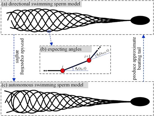
2.2.2. Construction of self-propelled sperm

The directional swimming sperm model can provide a valuable reference for building a self-propelled swimming model, which is necessary for studying the self-propelled behaviors in a complex flow environment. The construction of the self-propelled swimming sperm model is provided in Figure 2. First, we obtain a stable beating pattern within a beating cycle from the directional swimming sperm model (Figure 2(a)). Then, we extract and save the angles ($\theta \left(s_i,t\right)$ in Figure 2(b)) of all tail nodes at every moment as the expected angles. Finally, we construct a driving force to keep the actual angles following the corresponding expected angles all the time, and the beating pattern of self-propelled swimming sperm is achieved (Figure 2(c)).

Figure 2. Construction of the self-propelled swimming sperm model.

In the model, the joint force on the tail nodes is ${\mathit{F}}_T={\mathit{F}}_{\text{s}}+{\mathit{F}}_{\text{dr}}$, where ${\mathit{F}}_{\text{s}}$ is calculated by Equation (4), ${\mathit{F}}_{\text{dr}}$ is obtained by minimizing the difference of $\theta \left(s,t\right)$ and ${\theta }_{\text{e}}\left(s,t\right)$ as swimming. It is an exploratory step to synchronize $\theta \left(s,t\right)$ with ${\theta }_{\text{e}}\left(s,t\right)$ in a flow for the fluid resistance. Here, combining the theory of virtual work, we proposed a potential energy function as (16) $\begin{array}{rl}& {\mathit{W}}_{\text{T}}\left(s,t\right)\\ & ={\text{K}}_{\text{Tc}}\frac{5}{4}\sqrt[5]{{\left(\theta \left(s,t\right)-{\theta }_{\text{e}}\left(s,t\right)\right)}^4}\text{ sign}\left(\theta \left(s,t\right)-{\theta }_{\text{e}}\left(s,t\right)\right)\text{, }\end{array}$(16) where ${\text{K}}_{\text{Tc}}$ is the adjustment coefficient, it is set as $1\times {10}^{-10}\text{N}.\text{M}$. Based on which the tail beating pattern in Figure 2(c) is obtained. The binary sign function is set as $\text{sign}\left(x\right)=1\left(x>0\right),\text{sign}\left(x\right)=-1\left(x<0\right)$. Finally, Equation (7) is used to obtain ${\mathit{F}}_{\text{dr}}$.

Under the control of ${\mathit{F}}_T$, the tail beating of a self-propelled swimming sperm is achieved, as shown in Figure 2(c). Different from the directional swimming model, the bending force of the tail is independent of the real-time morphology of the tail itself, but is relevant to the angle $\theta \left(s,t\right)$. Our method makes the sperm be able to swim freely in a flow.

The above change also brings some other differences. By comparing Figure 2(a) and (c), we observe that their beating patterns are similar but distinguishable. The envelope formed by the beating tail in (c) is narrower than that in (a). Therefore, the propulsion velocity of the self-propelled swimming sperm is lower to some extent. Our results indicate that if putting the sperm at the centerline in Figure 1, the self-propelled model's propulsive efficiency is about 60% of the directional model. Moreover, due to the fluid resistance, the new model's beating pattern lags behind around 1/3 swing cycle compared with the directional model. Despite those differences, the swing patterns are similar and the swing periods are the same, so these factors will not essentially affect the motion law study of sperm.

2.3. The IB-LBM work-frame

Up to now, LBM has been widely used in fluid simulations (Bai et al., 2020; Chai & Shi, 2020; Gan et al., 2018; Li et al., 2016; Li et al., 2019). It has some appreciate advantages, such as fully parallelism, easy implementation of boundary conditions, and simple coding. In our simulation, the single relaxation lattice Boltzmann method (LBM) is used to simulate the flow field, and the D2Q9 lattice is applied. The corresponding discrete lattice Boltzmann equation is expressed as (Gan et al., 2019; Guo et al., 2002a; Ma et al., 2020) (17) $\begin{array}{rl}& g_i\left(\mathit{x}+\mathrm{\Delta }t,t+\mathrm{\Delta }t\right)-g_i\left(\mathit{x},t\right)\\ & =-\frac{1}{\tau }\left[g_i\left(\mathit{x},t\right)-g_i^{\text{eq}}\left(\mathit{x},t\right)\right]+\mathrm{\Delta }t{G}_i,\end{array}$(17) where $g_i\left(\mathit{x},t\right)$ is the probability density distribution function in the $e_i$ direction under $\mathit{x}$ at time $t$. $g_i^{\text{eq}}$ is the corresponding equilibrium distribution function, and $\tau$ is the dimensionless relaxation time. $G_i$ is an external force term. The mathematical formulas of $g_i^{\text{eq}}$ refers to (Ma et al., 2016; Wei et al., 2016). The wall boundary conditions are based on the non-equilibrium extrapolation method (Guo et al., 2002b).

The interaction model between the sperm and the flow is established by the immersed boundary method (IB) (Peskin, 2003). The gist of IB is to use a Delta distribution function $D\left(\mathit{x}-\mathit{X}\right)$ (Wang et al., 2017) to realize the exchange of the macroscopic physical quantity between the moving boundary nodes and background grid nodes. The main formulas are (Peskin, 2003): (18) $\begin{array}{rl}\mathit{f}\left(\mathit{x},t\right)& ={\int }_{\mathrm{\Gamma }}^{}\mathit{F}\left(s,t\right)D\left(\mathit{x}-\mathit{X}\right)\text{d}s,\end{array}$(18) (19) $\begin{array}{rl}\mathit{U}\left(s,t\right)& ={\int }_{\mathrm{\Omega }}^{}\mathit{u}\left(\mathit{x},t\right)D\left(\mathit{x}-\mathit{X}\right)\text{d}x,\end{array}$(19) Through Equation (18), the force $\mathit{F}$ received by the moving boundary nodes is applied to the fluid. By Equation (19), the velocity $\mathit{u}$ on the background grid nodes is assigned to the moving boundary nodes, so that their position is updated by $\mathit{U}\times \mathrm{\Delta }t$. Via such information exchange, IB and LBM are combined together (IB-LBM) to form a fluid-solid interaction numerical simulation framework. This framework is used to reveals the hydrodynamic mechanism of the sperm while swimming. This framework has been analyzed and demonstrated in (Liu et al., 2020), so we will not discuss the feasibility here again.

2.4. Validation and verification

2.4.1. Validation of the sperm propulsion by wall acceleration

In (Liu et al., 2020), we have quantitatively verified the propulsion law of traveling waves based on the IB-LBM. The result shows that the numerical method accurately describes the transmission law of a waving sheet with a low Reynolds number. This also indicates that the IB-LBM has an excellent capability to simulate sperm swimming in 2D cases effectively. In this paper, we modified the generating method of the swing tail, where the setting of the driving force for bending motion is changed. We conducted a contrast study between the directional swimming model (Liu et al., 2020) and the proposed self-propelled swimming model to verify its propulsive speed. In (Liu et al., 2020), the sperm could merely swim along a fixed line parallel to the wall. However, in the present model, the sperm can swim freely. If we want to control it to swim along a fixed line like the model in (Liu et al., 2020), just introduce an external force defined like $F_{\text{dis}}$ in Equation (8). So, in both models, the sperm can be set to swim along a given straight path.

To nondimensionalize the problem, the reference speed is ${\text{U}}_0=5\times {10}^{-4}$. $U_{x,t}^{\ast }$ is the propulsive speed in LBM, and its non-dimensional form is $U_{x,t}=U_{x,t}^{\ast }/{\text{U}}_0$. To measure the averaged propulsive speed within a period, a time-average propulsive speed ${\overline{U}}_{x,t}$ is defined as $\frac{1}{10T}{\int }_t^{t+10T}{U}_{x,t}\text{d}t.$ $\frac{({\overline{U}}_{x,t0+\text{T}}-{\overline{U}}_{x,t0})}{{\overline{U}}_{x,t0}}\times 100\mathrm{\%}<1\mathrm{\%}$ is the termination condition to obtain a stable ${\overline{U}}_{x,t0}$, which is marked simply by ${\overline{U}}_x$ as shown in Figure 3.

Figure 3. The average propulsive speed of directional and self-propelled swimming sperm.

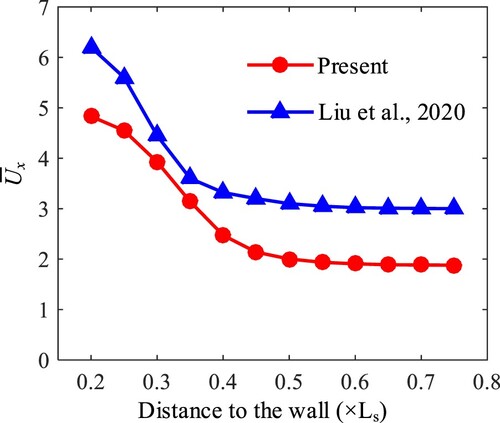
According to the results, two aspects are analyzed as the following. First, both the directional and self-propelled models produce similar wall accelerations. That is, for a sperm swimming parallel to a wall, its propulsive speed exhibits an increasing tendency as it approaches the wall (Qin et al., 2012). These results indicate that both two models can simulate sperm swimming correctly. Second, the self-propelled model produces a lower propulsion velocity compared with the directional model. We consider this is reasonable because the self-propelled model has a narrower envelope of the beating tail (as declared at the end of Sec 2.2), which means a lower propulsive force. To sum up, we believe the proposed self-propelled swimming sperm model is also valid to simulate the traveling wave propulsion of the sperm.

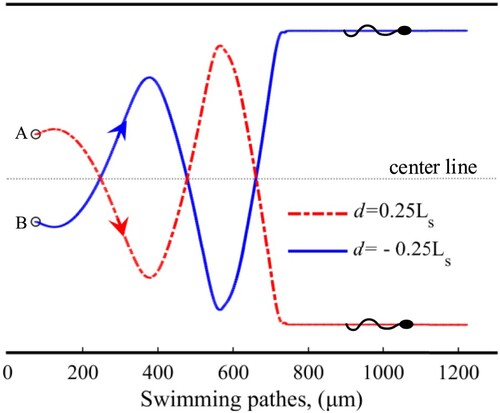
2.4.2. Verification of the symmetry of sperm motion

In this part, the symmetry of sperm motion is verified in a fluid between two parallel walls. In this model, the scale of the computational domain is $5{\text{L}}_{\text{s}}\times 2{\text{L}}_{\text{s}}$. Other parameters are set by referring to subsection 2.1. In Figure 4, a sperm is initialized horizontally at point A or B (they are both 0.25${\text{L}}_{\text{s}}$ to the centerline). The two points are mirror images of each other about the centerline. In theory, the swimming paths will also be mirror images about the centerline if the sperm motion is symmetric. According to the results in Figure 4, the symmetry of sperm motion is confirmed. That is, sperm may continuously swim forward unless there are some other factors to change its state.

Figure 4. Swimming paths used to verify the symmetry of sperm motion.

3. Results and discussion

3.1. A single sperm swims in Poiseuille flow

In this part, we studied the swimming of a single sperm in a confined space. The flow velocity, the inter-wall distance, and the initial position of the sperm are regulated to study the sperm's movement behavior. An external force is introduced to drive the fluid between the walls, thus establishing a Poiseuille flow. The theoretical value of maximum flow velocity $U_{\text{max}}$ in Poiseuille flow under a driving force $f_{\text{d}}$ can be calculated with Equation (1). To generate the Poiseuille flow with different $U_{max}$, a set of driving forces are varied by $f_{\text{d}0}=0\text{N}$, $f_{\text{d}1}=9.77\times {10}^{-18}\text{N}$, $f_{\text{d}2}=1.95\times {10}^{-17}\text{N}$, $f_{\text{d}3}=3.91\times {10}^{-17}\text{N}$, $f_{\text{d}4}=7.81\times {10}^{-17}\text{N}$ and $f_{\text{d}5}=1.56\times {10}^{-16}\text{N}$. In addition, five types of inter-wall distances are set as $W_{\text{c}1}=80\text{μ}\mathrm{m}$, $W_{\text{c}2}=110\text{μ}\mathrm{m}$, $W_{\text{c}3}=140\text{μ}\mathrm{m}$, $W_{\text{c}4}=170\text{μ}\mathrm{m}$, $W_{\text{c}5}=200\text{μ}\mathrm{m}$ respectively. To define the initial orientation of the sperm, the tail is free of bending force and in natural straightening state. We named the angle between the straight tail and the upper wall as orientation angle, marked with ${\theta }_{\text{a}}$ (${\theta }_{\text{a}}\in \left(-\pi ,\pi \right]$). In the present study, three orientation angles are considered, ${\theta }_{\text{a}1}=0$, ${\theta }_{\text{a}2}=\pi$ and ${\theta }_{\text{a}3}=-3\pi /80$. In addition, to locate the sperm, we used the front vertex of the sperm head to represent the position of the whole sperm; in the direction vertical to the wall, we defined −100% to 100% to describe the relative position from the bottom wall to the upper wall. And $d_1=-23\text{\%}$ and $d_2=-60.5$% are taken as the initial positions in simulations.

To express more clearly, we constructed a vector $M$ to declare different conditions, which includes four variables $x_1,x_2,x_3$ and $x_4$. The variable $x_1$ represents the driving force $f_d$; $x_2$ represents $W_{\text{c}}$; $x_3$ is the initial orientation angle of the sperm; $x_4$ refers to the initial position of the sperm. For example, $M\left(f_{\text{d}2},W_{\text{c}5},{\theta }_{\text{a}2},d_1\right)$ indicates the sperm swims under the following four conditions: $f_{\text{d}}=1.95\times {10}^{-17}\text{N}$, $W_{\text{c}}=200\text{μ}\mathrm{m}$, ${\theta }_{\text{a}}=\pi$, and $d=-23\mathrm{\%}\ast \frac{W_{\text{c}}}{2}=-23\text{μ}\mathrm{m}$. By changing the conditions of $M$ in the sperm behaviors simulation, four typical swimming patterns, including wall-adhesion, focusing, tumbling, and oscillating, were observed.

3.1.1. The four swimming patterns

3.1.1.1. Wall-adhesion pattern

When a sperm beats near a wall, it tends to attach to the wall and swims along with it stably. We named this pattern wall-adhesion swimming. This pattern is essentially resulted from the uneven lateral pressure distribution around the tail boundary, as has been studied in (Xu et al., 2018). Under the effect of the ‘repelling zone’ near the wall, the tail can still beat to some degree, keeping the sperm propelling during adhesion.

Figure 5(a) shows that at $M\left(f_{\text{d}0},W_{\text{c}5},{\theta }_{\text{a}3},d_1\right)$ and $M\left(f_{\text{d}0},W_{\text{c}5},{\theta }_{\text{a}3},d_2\right)$, sperms are captured eventually by the wall and form the wall-adhesion pattern. Similarly, Figure 5(b) exhibits the processes of wall-adhesion pattern at $M\left(f_{\text{d}1},W_{\text{c}5},{\theta }_{\text{a}3},d_1\right)$ and $M\left(f_{\text{d}2},W_{\text{c}5},{\theta }_{\text{a}3},d_1\right).$

Figure 5. The trajectories of sperms in the wall-adhesion pattern.

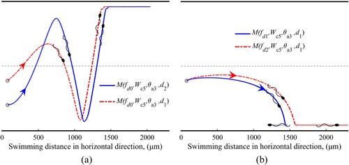
This figure indicates that the sperm can also form the wall-adhesion pattern in shear flow under certain conditions. From Figure 5, we know that the wall-adhesion pattern has relatively strong stability and can always be established in different initial positions or flows (in quiescent fluid or low-speed flow). These results are consistent with the ‘wall accumulation’ phenomena found for multiple sperms (Denissenko et al., 2012; Maude, 1963).

3.1.1.2. Focusing pattern

A focusing pattern describes that sperm swims stably at a particular position near the wall. Figure 6 shows the sperm trajectories in the focusing pattern under two different types of flows (flow shear rate). Unlike the wall-adhesion pattern, the sperm receives no influence of the ‘repelling zone’ in this pattern. The focused swimming phenomenon comes from the hydrodynamic balance near the wall.

Figure 6. Sperm trajectories in focusing pattern.

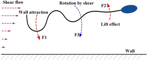
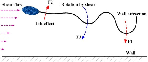
To understand the mechanism, an analysis is carried out below. As shown in Figure 7, a sperm in focused swimming mainly receives three types of forces, $F_1$,$F_2$ and $F_3$. $F_1$ comes from the tail beating. According to the setting of beating pattern (Figure 2), As the frontend (head and neck) of the sperm body is almost stiff during swimming, $F_1$ is mainly produced by the middle and distal parts of the tail (the swing parts of the sperm body). This force tends to make an anticlockwise rotation over the sperm body. $F_2$ denotes the lift force from the flow. As the sperm swims forward, it is found that the parts of the head and neck always keep a slight upwarp. This upwarp will result in a lift force to roll the sperm anticlockwise. $F_3$ represents the flow shear effect on the whole sperm body. It makes the sperm tend to perform a clockwise rotation. From Figure 6, we find that the equilibrium position of the sperm is closer to the wall at $f_{d2}$. This result indicates that the sperm in focused swimming tends to approach the wall as rising the shear rate. Therefore, there exists a confrontation between $F_{1,2}$(the joint result of $F_1$ and $F_2$) and $F_3$. If the confrontation reaches a balance, the sperm will keep steady swimming at a certain distance to the wall. In such a case, the focusing pattern comes into being.

Figure 7. Forces acting on a sperm in focusing pattern.

3.1.1.3. Tumbling pattern

The tumbling swimming pattern refers to a periodic tumbling phenomenon of sperm in a relatively high-shear-rate flow (Kumar & Ardekani, 2019). Figure 8 shows the trajectory of sperm in a tumbling swimming pattern at different shear strengths.

Figure 8. Sperm trajectories in the tumbling swimming pattern.

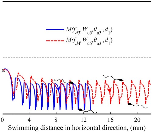
The causation of the tumbling swimming pattern can also be revealed by analyzing Figure 7. If we increase the flow shear rate when sperm is in the focusing pattern, the strength of $F_3$ will also rise. As the strength reaches a high enough level (by raising the driving force to $f_{\text{d}3}$ or $f_{\text{d}4}$), $F_1$ and $F_2$ can no longer constrain $F_3$, breaking the balance on the focused swimming and forming the tumbling pattern.

According to Figure 8, the tumbling sperm gets farther away from the adjacent wall at $f_{\text{d}4}$. That is, as promoting the flow shear, the sperm tends to apart from the adjacent wall. This result reveals an opposite trend from that in the focusing pattern.

3.1.1.4. Oscillating pattern

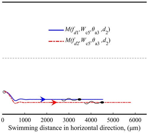
In the oscillating pattern, the sperm swims back and forth between walls due to relatively narrow space. Figure 9 shows the trajectory of sperm at $M\left(f_{\text{d}5},W_{\text{c}1},{\theta }_{\text{a}2},d_1\right)$ and $M\left(f_{\text{d}5},W_{\text{c}1},{\theta }_{\text{a}2},d_2\right)$, where the sperm swims periodically across the centerline between walls.

Figure 9. Sperm trajectories in the oscillating pattern.

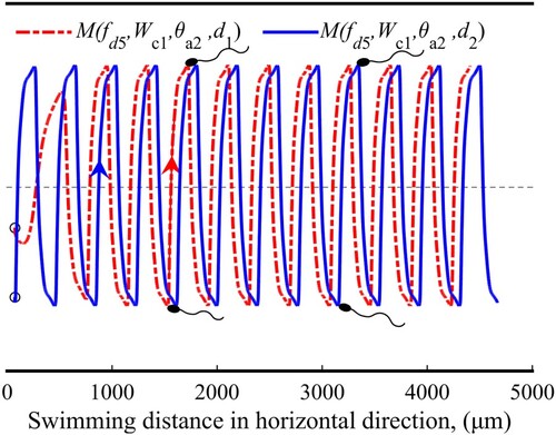
Figure 10 reveals the mechanism of the oscillating pattern. As the initial orientation angle of the sperm is ${\theta }_{\text{a}}={\theta }_{\text{a}2}=\pi$, $F_1$ to $F_3$ rotate the sperm clockwise, and make it have a tumbling trend. However, for the 80 µm inter-wall distance, after the sperm gets across the centerline, an opposite rotation works on it. Therefore, there is not enough space to turn around the sperm.

Figure 10. Formation of the oscillating pattern.

So in this case, the sperm looks continuously swim upstream. This interesting phenomenon was also reported in (Kumar & Ardekani, 2019), where a three-dimensional model is used.

Moreover, the latter section also reveals that in a relatively vast inter-wall distance, the oscillating pattern also happens even if the initial orientation angle ${\theta }_{\text{a}}=0$. We think that a relatively weak wall attraction mainly causes this pattern. As the sperm swims vertically to the wall, the wall attraction will almost disappear, which can be used to explain why the oscillating pattern is sensitive to the initial orientation.

3.1.2. Occurrence conditions of the swimming patterns

In Section 3.1.1, we have exhibited four patterns. In this section, we studied the occurrence law of swimming patterns in different conditions of $M\left(x_1,x_2,x_3,x_4\right)$. The settings of $x_1\text{to}{x}_4$ and the occurrence laws of swimming patterns are shown in Figure 11.

Figure 11. The occurrence laws of swimming patterns.

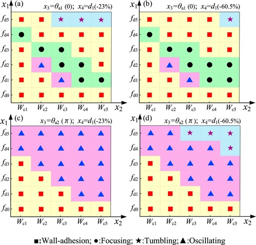
Through the settings of $x_1\text{to}{x}_4$ in Figure 11, the effects of $x_1\left(f_{\text{d}}\right)$ and $x_2\left(W_{\text{c}}\right)$ on the planar Poiseuille flow can be analyzed as below.

According to the Navier-Stokes equation, for the Poiseuille flow, there is $\frac{{\mathrm{\partial }}^2{u}_x}{\mathrm{\partial }{y}^2}=\frac{1}{\mu }\left(\frac{\mathrm{\partial }P}{\mathrm{\partial }x}-\rho f_{\text{d}}\right)$ and $\frac{\mathrm{\partial }P}{\mathrm{\partial }y}=0$, then we get $u_x=-\frac{1}{2\mu }\left(\rho f_d-\frac{\mathrm{\partial }P}{\mathrm{\partial }x}\right)\left(y^2-\frac{W_{\text{c}}^2}{4}\right)$, where the original point of $y$ is at the centerline between the two walls ($y\in \left[-0.5L_c,0.5L_c\right]$). In the present study, $\frac{\mathrm{\partial }P}{\mathrm{\partial }x}$ is set as 0 to satisfy the periodic flow conditions, so $u_x=-\frac{1}{2\mu }\left(\rho f_{\text{d}}\right)\left(y^2-\frac{W_{\text{c}}^2}{4}\right)$. Then, the shear force $F_{shear,y}=\mu \frac{\mathrm{\partial }{u}_x}{\mathrm{\partial }y}=-\rho f_{\text{d}}y$. This result indicates that the flow shear is in direct proportion to $f_{\text{d}}\text{ or }y$.

Based on the above analysis and Figure 11, there are four aspects summarized as the following. First, independent of initial states, the single sperm that swims in a quiescent fluid without flow shear will perform wall-adhesion swimming. Second, comparing the initial orientations with positions, the former has more influence on the final formation of swimming patterns. Third, the focusing and oscillating patterns are sensitive to the initial orientation. And they appear to happen in a particular range of flow shear. Forth, the tumbling pattern tends to occur in high shear flow cases.

3.2. Motion of sperm population

In (Mendiola et al., 2013), it is reported that the average density of sperm is about $5\times {10}^7$ in each ml. We calculate that each sperm occupies a cubic space with an edge length of $27\text{μ}\mathrm{m}$. Generally, the natural length of human sperm is about $55\text{μ}\mathrm{m}$ (Elgeti et al., 2015; Ishimoto & Gaffney, 2014; Nosrati et al., 2015). In theory, the sperm will inevitably come into contact with their neighboring sperm. Therefore, to simulate the motion of the sperm population, it is necessary to consider the interaction between sperms.

The default settings in Section 2.1 are applied in this section as well. In addition, a repulsive force $f_{\text{rs}}$ is assigned to control the distance between two neighboring sperms as they approach each other. The force is activated on the sperm tail nodes (not including the part inside the head area) and the head boundary nodes (not including the internal nodes), which is formularized as (20) $f_{\text{rs}}=\{\begin{array}{ll}{\text{K}}_{\text{rs}}({\displaystyle \frac{1}{e^{a\left(s-s_{\text{r}0}\right)}-1}}& \\ -{\displaystyle \frac{1}{e^{a\left(s_0-s_{\text{r}0}\right)}-1}})& s_{\text{r}0}<s\le s_0\\ 0& s>s_0\end{array},$(20) where ${\text{K}}_{\text{rs}}=1\times {10}^{-9}\text{N}.\text{m}$ is the rejection coefficient, $a=0.25$ is the empirical adjustment coefficient, and s is the distance between the boundary nodes of neighboring sperms. $s_{\text{r}0}=2.5\text{μ}\mathrm{m}$ is the lower limit of the distance s. $s_0=5\text{μ}\mathrm{m}$ is the cut-off distance of the repulsive force $f_{\text{rs}}$.

3.2.1. Sperm population swims in quiescent flow

In 1963, Lord studied the swimming behavior of bull sperm between a pair of coverslips with an inter-glass distance of 200 µm and proposed a formulation to describe the change of sperm distribution over time (Maude, 1963) (Rothschild, 1963). His study shows that most of the sperms tend to gather on the surface of the coverslips, which is also called wall accumulation, reflecting the ‘thigmotaxis’ (Ishimoto, 2017) (Magdanz et al., 2015). It has been widely known that the ‘thermotaxis’ and ‘chemotaxis’ are active behaviors of the sperm. Then, how about ‘thigmotaxis"? Whether the wall accumulation is a type of active behavior is still unknown and requires further investigation.

In this section, the motion of the sperm population is simulated, to explore the mechanism of wall accumulation. As shown in Figure 12(a), 16 sperms are initialized between a pair of coverslips, in which the inter-glass distance is 200 µm, same as the setting in (Maude, 1963) and (Rothschild, 1963).

Figure 12. The evolution of sperm distribution.

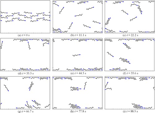
A 300 µm-length periodic channel is chosen as the computational domain, where the sperm can swim freely in a surrounding fluid. To mimic the realistic situation, the randomness and difference of sperm are considered in two aspects in the simulation. First, each sperm is given an initial inclination angle ($\frac{3}{80}\pi$ or $-\frac{3}{80}\pi$, Figure 12(a)) in the horizontal direction. Such settings express randomness on the sperms’ swimming direction. Second, the swing phase of the sperm tail is randomly assigned at a time interval of $\frac{1}{16}T$ ($T$ is the beating cycle), to represent the asynchronous tail beating.

The evolution of sperm distribution is shown in Figure 12(b-$i$). Firstly, the sperm between the two walls tends to adhere to and gather at the wall. Such wall accumulation phenomenon is consistent with the experimental results given in (Maude, 1963) and (Bukatin et al., 2020). Secondly, during the swimming process, an adsorption force arises between adjacent sperms in the same swimming direction. As a result, a phase lock is formed to obtain a relatively stable combination, which is also confirmed by experimental observations (Nosrati et al., 2015). Thirdly, the sperm that has formed a stable wall-adhesion pattern may leave the wall if other sperm approaches. Therefore, for the sperm population, the wall-adhesion pattern is just relatively stable. Figure 13 shows the movement trajectories of those sperms within 111.11 s.

Figure 13. The swimming trajectory of every individual sperm.

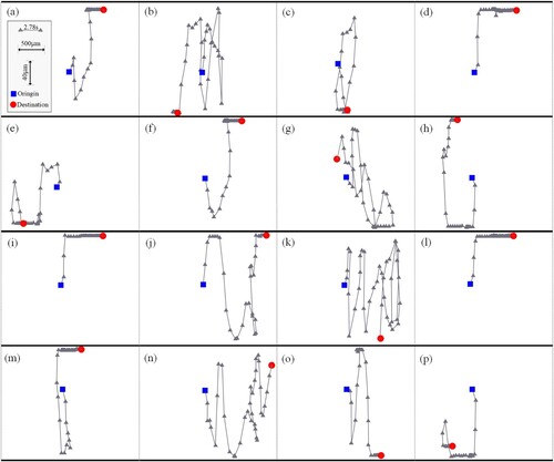
In this figure, the blue square represents the start position of the sperm, while the red circle represents the corresponding destination. On the trajectories, the time interval between two adjacent triangle markers is 2.78s. To display trajectories clearly, different spatial coordinate scales are applied in the $x$ and $y$ directions, as shown in the inset in Figure 13(a). In these trajectories, 14 cases formed relatively stable wall-adhesion at the end, except for (g) and (n). This means that most sperms in the population tend to be captured by the wall. Moreover, from the sub-figures (g,h,o), it is also observed that the wall-adhesion pattern can be broken under certain conditions. We think the underlying mechanism is collision and adsorption between sperms as swimming.

In this section, the simulation reveals that a sperm population swimming freely in a fluid tends to adhere to the wall, forming wall accumulation. These results prove that wall accumulation is mainly a passive behavior. Such behavior results from the evolution of hydrodynamic factors. We thus conclude that the ‘thigmotaxis’ of sperm is a type of passive behavior. By analyzing the formation of wall accumulation, it is found that two conditions are crucial. For condition (1), sperm has an opportunity to approach the wall in a confined space as long as no blockage is applied. For condition (2), the beating tail can be adsorbed on the wall surface (Xu et al., 2018).

To give a quantitative comparison, according to the method of Ref. (Rothschild, 1963), the statistical quantity of sperms within statistical intervals is displayed in Figure 14.

Figure 14. The distribution comparison of swimming sperms with other reports.

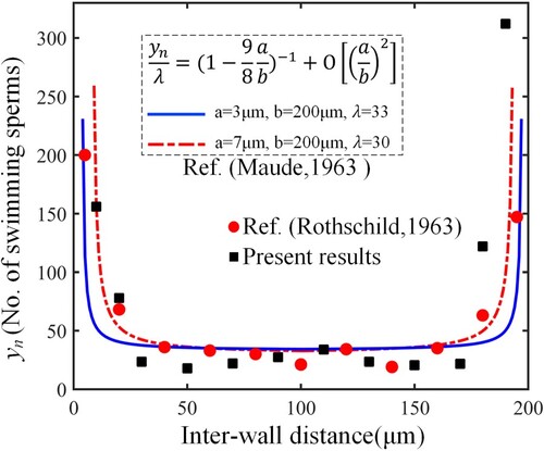
The theoretical curves are taken from the empirical formula of Ref. (Maude, 1963), where a is the minimum distance of the head to the surface, b is the distance between the two parallel surfaces, $\lambda$ is an adjustment coefficient. According to the reports, considering the average head size, the parameter combination of $a=3\text{μ}\mathrm{m}$ and $\lambda =33$ is reasonable to predict the sperm distribution. However, $a=7\text{μ}\mathrm{m}$ and $\lambda =30$ are better to fit their experimental observation. The present results are taken from three steps after 350 beating cycles (the swimming process is fully developed). (1) Count the sperm number within a space interval. For example, to get the data at 50$\text{μ}\mathrm{m}$ on the horizontal axis, the space interval is from 40$\text{μ}\mathrm{m}$ to 60$\text{μ}\mathrm{m}$. (2) Obtain the mean results from 10 moments with a time interval of 50 beating cycles. (3) Normalize all the sperm numbers in accordance with Ref. (Rothschild, 1963), and then generate the final results. From the comparison, our results are relatively close to the theoretical prediction and experimental observation.

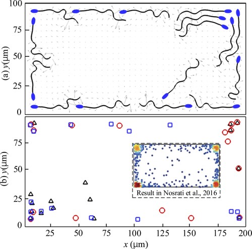
In addition, to study the sperm distribution in a closed rectangular cavity area, the above flow field boundaries are all changed as walls. The computational domain is resized to be $200\text{μ}\mathrm{m}\times 100\text{μ}\mathrm{m},$ just like one case in (Nosrati et al., 2016). The sperms are initialized randomly of their position and tail–head orientation around the center of the cavity area. Three cases labeled as 1–3 are carried out independently. All cases are stopped at the end of the 500th beating cycle. The actual distribution of the sperms is shown in Figure 15(a), and for all three cases, the final sperm distributions expressed by the front head vertexes are displayed in Figure 15(b). Figure 15 indicates that if sperms are put in a closed rectangular cavity area, the free-swimming sperms accumulate at the wall boundaries, especially at the corners. These results agree well with that in (Nosrati et al., 2016). Therefore, the above quantitative comparisons show that our model can simulate the distribution principles of free-swimming sperms near surfaces.

Figure 15. The swimming sperms in a closed rectangular cavity area. (a) The snapshot of sperms in case 2. (b) Sperm distribution of all the three cases. Case 1: red ‘○’; Case 2: black ‘▵’; Case 3: blue ‘□’.

3.2.2. Sperm population swims in Poiseuille flow

In this section, we studied the swimming of a sperm population in Poiseuille flow. A set of external driving forces are applied to drive the fluid to generate different flow velocities. Based on the current settings, the adjacent sperms may affect each other, and different Poiseuille flow velocities can make different distributions of sperms. Figure 16 displays the distributions of the sperm population at $t=111.11\text{s}$ under six types of driving forces ($f_{\text{d}0}$ to $f_{\text{d}5}$), as defined in Sec. 3.1. The initial position of the sperm is given in the inset (a1) in Figure 16(a), where eight sperms head to the left and the other eight head to the right.

Figure 16. The sperm and the pressure distribution in Poiseuille flow.

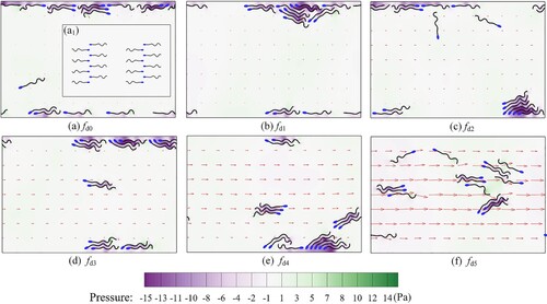
From Figure 16, the swimming characteristics of sperms can be summarized by their distribution and swimming direction. Firstly, sperms traveling at low flow velocity are more likely to adhere to the wall. For example, in cases (a-d), more than fourteen sperms gather at the wall in each case. In (e), ten sperms swim near the wall. However, in (f), almost no sperm gets close to the wall. These results show that the high velocity is not advantageous for the sperm to adhere to a wall. Secondly, we focus on the swimming direction. In (a), there are no evident characteristics of swimming direction. However, in (b-e), at least ten sperms swim upstream in each case. Especially in (b) and (d), all sixteen sperms swim upstream. The above results indicate that most sperms finally adhere to the wall and swim upstream for suitable flow velocities regardless of the sperm's initial direction. This is the typical ‘rheotaxis’ of the sperm. So, our study reveals that the occurrence of sperm rheotaxis requires some specific conditions.

In addition, we also defined the pressure index. In LBM, $P^{\ast }=c_s^2\left({\rho }^{\ast }-1\right)$, where $P^{\ast }$ is the non-dimensional pressure and ${\rho }^{\ast }$ is the non-dimensional density. Then, $P^{\ast }$ can be transferred in physical unit by $P=P^{\ast }\times \frac{m_{\text{r}}}{L_{\text{r}}\mathrm{\Delta }{t}_{\text{r}}^2}$ with $m_{\text{r}}={\rho }_{\text{r}}{L}_{\text{r}}^3$. Where $m_{\text{r}}$, $L_{\text{r}}$, $\mathrm{\Delta }{t}_{\text{r}}$ and ${\rho }_{\text{r}}$ are the physical units, which correspond to the mass, grid spacing, time step and density. In the simulation, ${\rho }_{\text{r}}=1000\text{kg}/{\text{m}}^3$, $L_{\text{r}}=2.5\times {10}^{-7}\text{m}$ and $\mathrm{\Delta }{t}_{\text{r}}=5\times {10}^{-8}\text{s}$. By observing the pressure distribution chromaticity diagram, it is found that negative pressure will appear between two adjacent sperms or between the sperm and the wall as the sperm tail swings. Such negative pressure can make a mutual attraction between nearby boundaries, resulting in the wall-adhesion or sperm gathering phenomenon.

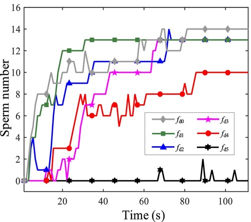
To study the process of sperm wall-adhesion behavior, we counted the number of sperms swimming adherently in Figure 17. If the distance between the front vertex of the sperm head and the wall is less than $17.5\text{μ}\mathrm{m}$ (marked with $s_{\text{c}}\le 17.5\text{μ}\mathrm{m}$, it is about $\frac{1}{3}{\text{L}}_{\text{s}}$), this sperm is regarded as being in the state of wall-adhesion. Figure 17 shows that wall-adhesion behavior mainly occurs, as the flow velocity is relatively low. Moreover, with the increase of the flow speed, the sperm number in the wall-adhesion state decreases.

Figure 17. The number of sperms that swim adherently.

In addition, in the case with $f_{\text{d}3}$, we notice that a single sperm tends to appear tumbling swimming. However, for multiple sperms, more sperms achieve to behave stably to adhered to a wall, which shows that the interaction between sperms promotes wall-adhesion.

In the next, the rheotaxis is discussed. In the fertilization process, it is crucial for a sperm to follow the right way to the egg. This makes the sperm have to perform upward swimming, that is, the phenomenon of rheotaxis. It is a fascinating topic that how the sperm to distinguish the flow direction. Some recent studies indicated that the flow shear near the wall is the primary causation of rheotaxis, and the rheotaxis is essentially a passive phenomenon (Zhang et al., 2016) (Ishimoto, 2017). In this paper, we focus on the rheotaxis of the sperm population.

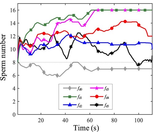
To study the swimming direction in a directional flow, we counted the number of sperms swimming upstream (also with $s_{\text{c}}\le 17.5\text{μ}\mathrm{m}$) in Figure 18. The swimming direction is only divided bidirectionally into left and right (upstream and downstream). We take the orientation of the sperm head as the swimming direction of the sperm, by identifying the relative positions of the two vertexes on the long axis of the sperm head. Figure 18 shows that flow velocity has an essential impact on the direction of sperm swimming. Furthermore, an appropriate flow velocity may be significant to induct more sperms swimming upstream. For the cases $f_{\text{d}1}$ and $f_{\text{d}3}$, all sixteen sperms keep swimming upstream. However, there are six sperms swimming downstream for the case $f_{\text{d}2}$. This is because some sperms have established the wall-adhesion at the beginning, and such a pattern is hard to break. (The wall-adhesion in 3D case is not so steady, the reason is analyzed as the limitation of the 2D model in the end of this paper). Therefore, in the 2D model, the initialization of the sperm population can also affect the final statistics of swimming direction.

Figure 18. The number of sperms that swim upstream.

3.2.3 Propulsion of multi-sperm combination

In the simulation of sperm population swimming, several types of the multi-sperm combination were observed due to the mutual adsorption of the adjacent sperms. Such phenomena can also be appreciated in some experiments (Nosrati et al., 2015). Therefore, it is interesting to study the combining form of sperms and its propulsive speed. In this section, as shown in Figure 19, two control modes ((a) and (b)) and five combining forms ((c-g)) are set to study the propulsive speed of sperm combinations.

Figure 19. Snapshots of control modes (a, b) and combining forms of three sperms (c-g).

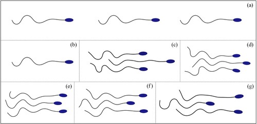
The settings are listed below. (1) sperm head's front vertex is fixed at a given horizontal line with an external force defined like $F_{\text{dis}}$ in Equation (8). All sperms are set to swim freely along the corresponding horizontal lines, where a distance $s_{\text{g}}$ is applied between two adjacent lines. (2) The reason that three sperms are used to establish the combining form is to make the swimming direction to be parallel to the wall. (3) In (a) and (b), the front vertex of the sperm head is restricted on the centerline between the walls. The sperm is set swimming along the centerline. In (c-g), the front vertex on the head of the middle sperm is also restricted on the centerline. (4) The results in (c-g) reveal that under the effects of mutual adsorption and phase locking, some stable combining forms can be obtained, which may contain different propulsive speeds.

A time scope of 360 beating cycles is chosen to simulate the swimming process. To measure the propulsive speed of each case, a time-average propulsive speed ${\overline{U}}_x=\frac{1}{n}\sum _{i=1}^n\left(\frac{1}{10T}{\int }_t^{t+10T}{U}_{x,i,t}dt\right)$ is defined, where $U_{x,i,t}$ is the horizontal ($x$) speed of the $i-\text{th}$ sperm, $n$ is the sperm number in the combination. Select $s_{\text{g}}=6\text{μ}\mathrm{m}$, and to make the sperms swim in parallel as possible as they swim together, set $s_{\text{r}0}=2.5\text{μ}\mathrm{m}$ and $s_0=5\text{μ}\mathrm{m}$ in Equation (20) to control the distance between sperms. Figure 20 shows the average propulsive speed ${\overline{U}}_x$ of the control modes and combining forms.

Figure 20. ${\overline{U}}_x$ of the control modes and combining forms. µm/s.

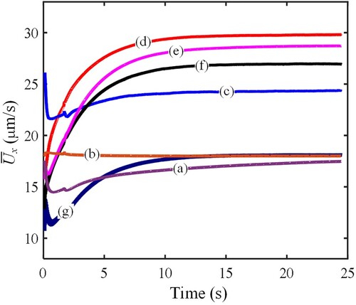
By comparing Figure 20(a) with (b), the propulsive speed of the in-line swimming sperms is not faster than that of a single sperm. This is an interesting result showing that the propulsive speed is not enhanced, although it seems that three sperms swimming in-line may accumulate propulsive force. The possible reason is given below. Due to the low Reynolds number, the viscous effect is the dominant factor to propulsion. The impact of the sperm on the fluid is just in a limited scope around the sperm boundary. As they swim in-line, there is little cooperative advantage. Moreover, we also observed that the propulsive speed of sperm in (a) is slightly lower than that in (b). We think this is because the sperm head is restricted in the vertical direction, changing the flow and further affecting the propulsive speed.

In addition, the propulsive speed of sperms in (a) experiences a long time to reach a relatively steady level. This is caused by the horizontal spacing adjustment between adjacent sperms. In this process, the spacing between every two adjacent sperms gradually evolves to be equal.

All combining forms, except case (g), can generate faster propulsive speed than a single sperm. These results indicate that most sperm combinations can help to promote propulsive speed. Meanwhile, it is also found that there are some distinct differences in the propulsion as the combining form changes. Case (d) is the fastest, followed by (e), (f) and (c); case (g) is the slowest in the five combining forms.

As to the different combining forms, they correspond to different propulsive speeds. Firstly, for case (d), we think two primary reasons make it the faster case. The one is that the three sperms construct a wedge shape. Such a shape is beneficial to reduce fluid resistance. The other is we observe that the beating amplitudes of all sperms not decreased. This will not slow down the propulsion of each single, as well as the combination. Secondly, in case (e), a shield shape is formed by the three sperms. Such a shape will produce a more considerable fluid resistance than the wedge shape. Therefore, although the tail beating is sufficient, the propulsive speed is lower than case (d). Finally, a similar analysis can also be used to explain the propulsive speed level in other cases. The propulsive speed in case (g) is remarkedly reduced. This is because the tail beatings of the lateral two sperms are both restricted by the middle sperm, causing the low propulsion.

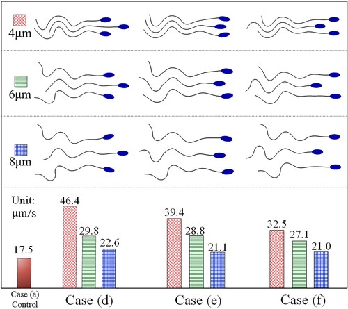
Here, the distance $s_g=6\text{μ}\mathrm{m}$, it is a presetting parameter, which may affect the propulsion of sperm combination. To discuss the detailed influences, we picked up the three fastest swimming modes (d), (e), and (f) in Figure 20. Then change $s_{\text{g}}$ to be 4 and 8 µm, respectively. To make the sperms to swim in parallel as possible in each case, in Equation (20), we set $s_{\text{r}0}=0.5\text{μ}\mathrm{m}$ and $s_0=3\text{μ}\mathrm{m}$ for $s_{\text{g}}=4$ µm, and set $s_{\text{r}0}=4.5\text{μ}\mathrm{m}$ and $s_0=7\text{μ}\mathrm{m}$ for $s_g=8$ µm. The corresponding sperm combinations at the 360 beating cycles and their propulsive speeds ${\overline{U}}_x$ are displayed in Figure 21. The results indicate that a narrower combining distance between adjacent sperms is more advantageous for enhancing the propulsive speed. The wedge-shaped combination form is the best way to obtain the optimal swimming speed.

Figure 21. The propulsive speed under different combining distances.

In brief, four aspects are summarized as the following according to the above analysis. (1) When multiple sperms are swimming in a line, the propulsive speed of these sperms may not be faster than a single sperm case. (2) For different combinations, the wedge-shaped form is better than others for less fluid resistance to enhance the propulsive speed. (3) The adsorption between adjacent sperms may restrict the tail beating of each other. A sufficient tail beating is better for promoting the propulsive speed. (4) A narrower combining distance between adjacent sperms is better to promote the propulsive speed.

4. Conclusion remarks

The distribution, rheotaxis and propulsion of sperms in confined flows have been explored by using an improved self-propelled sperm model based on the immersed boundary-lattice Boltzmann method. First, the swimming patterns of a single sperm in the Poiseuille flow have been studied by changing the flow velocity, inter-wall distance, and initial positions of the sperm. Four swimming patterns, including wall-adhesion, focusing, tumbling and oscillating cases, have been observed and discussed in detail. Multiple sperms swimming in confined flows have then been studied. Sixteen sperms are considered. It is found that the sperm rheotaxis could be enhanced if the counter flow speed increases in a particular scope. Moreover, the collision and adsorption between adjacent sperms can facilitate sperms attracted by the wall. Finally, two control patterns and five combining forms are set to investigate the corresponding propulsive speed. Our results show that some sperm combinations can promote propulsive speed remarkably, and a narrower combining distance is better to promote the propulsive speed.

It is noted that the 2D model has its limitations. In the actual 3D cases, sperm can swim in a spiral motion. It may perform attached swimming as approaching a wall, but the 2D model can't do this. In addition, the beating tail in 2D is like a waving flat surface, which will generate a larger propulsive force than the 3D tail. Therefore, the 2D model is not suitable for measuring sperm speed quantitatively. However, despite the above problems, the 2D model can simulate some phenomena of sperm behaviors, as exhibited in this paper. It can provide some insights to help us to understand the mechanism in sperm motion. In the future, as a follow-up to the present study, we plan to develop a 3D sperm model to investigate the mysteries in sperm propulsion, sperm interaction, and sperm navigation (i.e. rheotaxis, chemotaxis, etc.).

Disclosure statement

No potential conflict of interest was reported by the author(s).

Additional information

Funding

This work is supported by the National Natural Science Foundation of China (grant no 82172066 and 81771935) and the Australian Research Council (grant no DE160101098).

References

- Bahat, A., Caplan, S. R., & Eisenbach, M. (2012). Thermotaxis of human sperm cells in extraordinarily shallow temperature gradients over a wide range. PLoS One, 7(7), e41915. https://doi.org/10.1371/journal.pone.0041915
- Bai, X.-D., Zhang, W., & Wang, Y. (2020). Deflected oscillatory wake pattern behind two side-by-side circular cylinders. Ocean Engineering, 197, https://doi.org/10.1016/j.oceaneng.2019.106847
- Boryshpolets, S., Perez-Cerezales, S., & Eisenbach, M. (2015). Behavioral mechanism of human sperm in thermotaxis: A role for hyperactivation. Human Reproduction, 30(4), 884–892. https://doi.org/10.1093/humrep/dev002
- Bukatin, A., Denissenko, P., & Kantsler, V. (2020). Self-organization and multi-line transport of human spermatozoa in rectangular microchannels due to cell-cell interactions. Scientific Reports, 10(1), 9830. https://doi.org/10.1038/s41598-020-66803-2
- Campuzano, S., Esteban-Fernandez de Avila, B., Yanez-Sedeno, P., Pingarron, J. M., & Wang, J. (2017). Nano/microvehicles for efficient delivery and (bio)sensing at the cellular level. Chemical Science, 8(10), 6750–6763. https://doi.org/10.1039/c7sc02434g
- Chai, Z., & Shi, B. (2020). Multiple-relaxation-time lattice Boltzmann method for the Navier-Stokes and nonlinear convection-diffusion equations: Modeling, analysis, and elements. Physical Review E, 102(2-1), 023306. https://doi.org/10.1103/PhysRevE.102.023306
- Cortez, R., Fauci, L., & Medovikov, A. (2005). The method of regularized stokeslets in three dimensions: Analysis, validation, and application to helical swimming. Physics of Fluids, 17(3), 031504. https://doi.org/10.1063/1.1830486
- Denissenko, P., Kantsler, V., Smith, D. J., & Kirkman-Brown, J. (2012). Human spermatozoa migration in microchannels reveals boundary-following navigation. Proceedings of the National Academy of Sciences, 109(21), 8007–8010. https://doi.org/10.1073/pnas.1202934109
- Dillon, R., & Zhuo, J. (2010). Using the immersed boundary method to model complex fluids-structure interaction in sperm motility. Discrete and Continuous Dynamical Systems - Series B, 15(2), 343–355. https://doi.org/10.3934/dcdsb.2011.15.343
- Elgeti, J., Kaupp, U. B., & Gompper, G. (2010). Hydrodynamics of sperm cells near surfaces. Biophysical Journal, 99(4), 1018–1026. https://doi.org/10.1016/j.bpj.2010.05.015
- Elgeti, J., Winkler, R. G., & Gompper, G. (2015). Physics of microswimmers–single particle motion and collective behavior: A review. Reports on Progress in Physics, 78(5), 056601. https://doi.org/10.1088/0034-4885/78/5/056601
- Fisher, H. S., Giomi, L., Hoekstra, H. E., & Mahadevan, L. (2014). The dynamics of sperm cooperation in a competitive enviro·ent. Proceedings of the Royal Society B: Biological Sciences, 281, 1790. https://doi.org/10.1098/rspb.2014.0296
- Friedrich, B. M., Riedel-Kruse, I. H., Howard, J., & Julicher, F. (2010). High-precision tracking of sperm swimming fine structure provides strong test of resistive force theory. Journal of Experimental Biology, 213(Pt 8), 1226–1234. https://doi.org/10.1242/jeb.039800
- Gadêlha, H., Hernández-Herrera, P., Montoya, F., Darszon, A., & Corkidi, G. (2020). Human sperm uses asymmetric and anisotropic flagellar controls to regulate swimming symmetry and cell steering. Science Advances, 6(31), eaba5168. https://doi.org/10.1126/sciadv.aba5168
- Gan, Y., Xu, A., Zhang, G., Zhang, Y., & Succi, S. (2018). Discrete Boltzmann trans-scale modeling of high-speed compressible flows. Physical Review E, 97(5-1), 053312. https://doi.org/10.1103/PhysRevE.97.053312
- Gan, Y.-B., Xu, A.-G., Zhang, G.-C., Lin, C.-D., Lai, H.-L., & Liu, Z.-P. (2019). Nonequilibrium and morphological characterizations of kelvin–helmholtz instability in compressible flows. Frontiers of Physics, 14(4), https://doi.org/10.1007/s11467-019-0885-4
- Ghalandari, M., Mirzadeh Koohshahi, E., Mohamadian, F., Shamshirband, S., & Chau, K. W. (2019). Numerical simulation of nanofluid flow inside a root canal. Engineering Applications of Computational Fluid Mechanics, 13(1), 254–264. https://doi.org/10.1080/19942060.2019.1578696
- Guo, Z., Zheng, C., & Shi, B. (2002a). Discrete lattice effects on the forcing term in the lattice Boltzmann method. Physical Review E, 65(4 Pt 2B), 046308. https://doi.org/10.1103/PhysRevE.65.046308
- Guo, Z., Zheng, C., & Shi, B. (2002b). An extrapolation method for boundary conditions in lattice Boltzmann method. Physics of Fluids, 14(6), 2007–2010. https://doi.org/10.1063/1.1471914
- Hyakutake, T., Sato, K., & Sugita, K. (2019). Study of bovine sperm motility in shear-thinning viscoelastic fluids. Journal of Biomechanics, 88, 130–137. https://doi.org/10.1016/j.jbiomech.2019.03.035
- Ishimoto, K. (2017). Guidance of microswimmers by wall and flow: Thigmotaxis and rheotaxis of unsteady squirmers in two and three dimensions. Physical Review E, 96(4-1), 043103. https://doi.org/10.1103/PhysRevE.96.043103
- Ishimoto, K., Cosson, J., & Gaffney, E. A. (2016). A simulation study of sperm motility hydrodynamics near fish eggs and spheres. Journal of Theoretical Biology, 389, 187–197. https://doi.org/10.1016/j.jtbi.2015.10.013
- Ishimoto, K., & Gaffney, E. A. (2014). A study of spermatozoan swimming stability near a surface. Journal of Theoretical Biology, 360, 187–199. https://doi.org/10.1016/j.jtbi.2014.06.034
- Ishimoto, K., & Gaffney, E. A. (2015). Fluid flow and sperm guidance: A simulation study of hydrodynamic sperm rheotaxis. Journal of The Royal Society Interface, 12(106), https://doi.org/10.1098/rsif.2015.0172
- Ishimoto, K., & Gaffney, E. A. (2017). Boundary element methods for particles and microswimmers in a linear viscoelastic fluid. Journal of Fluid Mechanics, 831, 228–251. https://doi.org/10.1017/jfm.2017.636
- Ishimoto, K., & Gaffney, E. A. (2018). Hydrodynamic clustering of human sperm in viscoelastic fluids. Scientific Reports, 8(1), 15600. https://doi.org/10.1038/s41598-018-33584-8
- Kantsler, V., Dunkel, J., Blayney, M., & Goldstein, R. E. (2014). Rheotaxis facilitates upstream navigation of mammalian sperm cells. Elife, 3, e02403. https://doi.org/10.7554/eLife.02403
- Kumar, M., & Ardekani, A. M. (2019). Effect of external shear flow on sperm motility. Soft Matter, 15(31), 6269–6277. https://doi.org/10.1039/c9sm00717b
- Li, D., Lai, H., & Lin, C. (2019). Mesoscopic simulation of the Two-Component System of coupled sine-gordon equations with lattice Boltzmann method. Entropy (Basel), 21(6), https://doi.org/10.3390/e21060542
- Li, Q., Kang, Q. J., Francois, M. M., & Hu, A. J. (2016). Lattice Boltzmann modeling of self-propelled leidenfrost droplets on ratchet surfaces. Soft Matter, 12(1), 302–312. https://doi.org/10.1039/c5sm01353d
- Liu, Q.-Y., Tang, X.-Y., Chen, D.-D., Xu, Y.-Q., & Tian, F.-B. (2020). Hydrodynamic study of sperm swimming near a wall based on the immersed boundary-lattice Boltzmann method. Engineering Applications of Computational Fluid Mechanics, 14(1), 853–870. https://doi.org/10.1080/19942060.2020.1779134
- Ma, J., Wang, Z., Young, J., Lai, J. C. S., Sui, Y., & Tian, F.-B. (2020). An immersed boundary-lattice Boltzmann method for fluid-structure interaction problems involving viscoelastic fluids and complex geometries. Journal of Computational Physics, 415, 109487. https://doi.org/10.1016/j.jcp.2020.109487
- Ma, J. T., Xu, Y. Q., & Tang, X. Y. (2016). A numerical simulation of cell separation by simplified asymmetric pinched flow fractionation. Computational and Mathematical Methods in Medicine, 2016, 2564584. https://doi.org/10.1155/2016/2564584
- Magdanz, V., Koch, B., Sanchez, S., & Schmidt, O. G. (2015). Sperm dynamics in tubular confinement. Small, 11(7), 781–785. https://doi.org/10.1002/smll.201401881
- Magdanz, V., Medina-Sanchez, M., Schwarz, L., Xu, H., Elgeti, J., & Schmidt, O. G. (2017). Spermatozoa as functional components of robotic microswimmers. Advanced Materials, 29, 24. https://doi.org/10.1002/adma.201606301
- Maude, A. D. (1963). Non-random Distribution of Bull Spermatozoa in a Drop of Sperm suspension. Nature, 200(4904), 381. https://doi.org/10.1038/200381a0
- Mendiola, J., Jørgensen, N., Mínguez-Alarcón, L., Sarabia-Cos, L., López-Espín, J. J., Vivero-Salmerón, G., Ruiz-Ruiz, K. J., Fernández, M. F., Olea, N., Swan, S. H., & Torres-Cantero, A. M. (2013). Sperm counts may have declined in young university students in southern Spain. Andrology, 1(3), 408–413. https://doi.org/10.1111/j.2047-2927.2012.00058.x
- Nosrati, R., Driouchi, A., Yip, C. M., & Sinton, D. (2015). Two-dimensional slither swimming of sperm within a micrometre of a surface. Nature Communications, 6(1), 8703. https://doi.org/10.1038/ncomms9703
- Nosrati, R., Graham, P. J., Liu, Q., & Sinton, D. (2016). Predominance of sperm motion in corners. Scientific Reports, 6(1), 26669. https://doi.org/10.1038/srep26669
- Omori, T., & Ishikawa, T. (2016). Upward swimming of a sperm cell in shear flow. Physical Review E, 93(3), 032402. https://doi.org/10.1103/PhysRevE.93.032402
- Peskin, C. S. (2003). The immersed boundary method. Acta Numerica, 11, 479–517. https://doi.org/10.1017/s0962492902000077
- Qin, F.-H., Huang, W.-X., & Sung, H. J. (2012). Simulation of small swimmer motions driven by tail/flagellum beating. Computers & Fluids, 55, 109–117. https://doi.org/10.1016/j.compfluid.2011.11.006
- Ramírez-Gómez, H. V., Sabinina, V. J., Pérez, M. V., Beltran, C., Carneiro, J., Wood, C. D., Tuval, I., Darszon, A., & Guerrero, A. (2020). Sperm chemotaxis is driven by the slope of the chemoattractant concentration field. Elife, 9, e50532. https://doi.org/10.7554/eLife.50532
- Rothschild, L. (1963). Non-random Distribution of Bull Spermatozoa in a Drop of Sperm suspension. Nature, 198(4886), 1221. https://doi.org/10.1038/1981221a0
- Salih, S. Q., Aldlemy, M. S., Rasani, M. R., Ariffin, A. K., Ya, T. M. Y. S. T., Al-Ansari, N., Yaseen, Z. M., & Chau, K. W. (2019). Thin and sharp edges bodies-fluid interaction simulation using cut-cell immersed boundary method. Engineering Applications of Computational Fluid Mechanics, 13(1), 860–877. https://doi.org/10.1080/19942060.2019.1652209
- Schiffer, C., Rieger, S., Brenker, C., Young, S., Hamzeh, H., Wachten, D., Tüttelmann, F., Röpke, A., Kaupp, U. B., Wang, T., & Wagner, A. (2020). Rotational motion and rheotaxis of human sperm do not require functional CatSper channels and transmembrane Ca(2+) signaling. The EMBO Journal, 39(4), e102363. https://doi.org/10.15252/embj.2019102363
- Seandel, M., & Rafii, S. (2011). In vitro sperm maturation. Nature, 471(7339), 453–455. https://doi.org/10.1038/471453a
- Smith, D. J., Gaffney, E. A., Blake, J. R., & Kirkman-Brown, J. C. (2009). Human sperm accumulation near surfaces: A simulation study. Journal of Fluid Mechanics, 621, 289–320. https://doi.org/10.1017/s0022112008004953
- Strunker, T., Goodwin, N., Brenker, C., Kashikar, N. D., Weyand, I., Seifert, R., & Kaupp, U. B. (2011). The CatSper channel mediates progesterone-induced Ca2+ influx in human sperm. Nature, 471(7338), 382–386. https://doi.org/10.1038/nature09769
- Sun, D.-K., Jiang, D., Xiang, N., Chen, K., & Ni, Z.-H. (2013). An immersed boundary-lattice Boltzmann simulation of particle hydrodynamic focusing in a straight microchannel. Chinese Physics Letters, 30(7), 074702. https://doi.org/10.1088/0256-307x/30/7/074702
- Thapa, S., & Heo, Y. S. (2019). Microfluidic technology for in vitro fertilization (IVF). JMST Advances, 1(1-2), 1–11. https://doi.org/10.1007/s42791-019-0011-3
- Tian, F.-B., Luo, H., Song, J., & Lu, X.-Y. (2013). Force production and asymmetric deformation of a flexible flapping wing in forward flight. Journal of Fluids and Structures, 36, 149–161. https://doi.org/10.1016/j.jfluidstructs.2012.07.006
- Tian, F.-B., & Wang, L. (2021). Numerical modeling of sperm swimming. Fluids, 6(73), 6020073. https://doi.org/10.3390/fluids6020073
- Tian, F. B., Young, J., & Lai, J. C. S. (2016). An immersed boundary-lattice Boltzmann method for swimming sperms. The 20th Australasian Fluid Mechanics Conference Perth,; December 05-08; Western Australia., Western Australia.
- Wagenaar, B. D., Geijs, D. J., Boer, H. L. D., Bomer, J. G., Olthuis, W., Berg, A. V. D., & Segerink, L. I. (2016). Spermometer: Electrical characterization of single boar sperm motility. Fertility and Sterility, 106(3), 773–780. https://doi.org/10.1016/j.fertnstert.2016.05.008
- Wang, L., Currao, G. M. D., Han, F., Neely, A. J., Young, J., & Tian, F.-B. (2017). An immersed boundary method for fluid–structure interaction with compressible multiphase flows. Journal of Computational Physics, 346, 131–151. https://doi.org/10.1016/j.jcp.2017.06.008
- Wei, Q., Xu, Y.-Q., Tang, X.-Y., & Tian, F.-B. (2016). An IB-LBM study of continuous cell sorting in deterministic lateral displacement arrays. Acta Mechanica Sinica, 32(6), 1023–1030. https://doi.org/10.1007/s10409-016-0566-2
- Wei, Q., Xu, Y. Q., Tian, F. B., Gao, T. X., Tang, X. Y., & Zu, W. H. (2014). IB-LBM simulation on blood cell sorting with a micro-fence structure. Bio-Medical Materials and Engineering, 24(1), 475–481. https://doi.org/10.3233/BME-130833
- Woolley, D. M., Crockett, R. F., Groom, W. D., & Revell, S. G. (2009). A study of synchronisation between the flagella of bull spermatozoa, with related observations. Journal of Experimental Biology, 212(Pt 14), 2215–2223. https://doi.org/10.1242/jeb.028266
- Xu, H., Medina-Sánchez, M., Magdanz, Schwarz, L., Hebenstreit, F., & Schmidt, O. G. (2018). Sperm-hybrid micromotor for targeted drug delivery. ACS Nano, 12(1), 327–337. https://doi.org/10.1021/acsnano.7b06398
- Xu, Y.-Q., Jiang, Y.-Q., Wu, J., Sui, Y., & Tian, F.-B. (2017). Benchmark numerical solutions for two-dimensional fluid–structure interaction involving large displacements with the deforming-spatial-domain/stabilized space–time and immersed boundary–lattice Boltzmann methods. Proceedings of the Institution of Mechanical Engineers, Part C: Journal of Mechanical Engineering Science, 232(14), 2500–2514. https://doi.org/10.1177/0954406217723942
- Xu, Y.-Q., Wang, M.-Y., Liu, Q.-Y., Tang, X.-Y., & Tian, F.-B. (2018). External force-induced focus pattern of a flexible filament in a viscous fluid. Applied Mathematical Modelling, 53, 369–383. https://doi.org/10.1016/j.apm.2017.09.001
- Yang, Y., Elgeti, J., & Gompper, G. (2008). Cooperation of sperm in two dimensions: Synchronization, attraction, and aggregation through hydrodynamic interactions. Physical Review E, 78(6 Pt 1), 061903. https://doi.org/10.1103/PhysRevE.78.061903
- Yin, B., & Luo, H. (2010). Effect of wing inertia on hovering performance of flexible flapping wings. Physics of Fluids, 22(11), 111902. https://doi.org/10.1063/1.3499739
- Zhang, Z., Liu, J., Meriano, J., Ru, C., Xie, S., Luo, J., & Sun, Y. (2016). Human sperm rheotaxis: A passive physical process. Scientific Reports, 6(1), 23553. https://doi.org/10.1038/srep23553
- Zhu, L., & Peskin, C. S. (2002). Simulation of a flapping flexible filament in a flowing soap film by the immersed boundary method. Journal of Computational Physics, 179(2), 452–468. https://doi.org/10.1006/jcph.2002.7066