Aerodynamic performance of traveling road vehicles on a single-level rail-cum-road bridge under crosswind and aerodynamic impact of traveling trains

ABSTRACT

Crosswind and train-induced wind are major factors influencing the aerodynamic performance of vehicles on single-level rail-cum-road bridges. Based on computational fluid dynamics (CFD) technology, this work developed a numerical model to discuss relevant issues. The flow features of the vehicle-bridge system, the influence of different lanes and vehicles are explored, and the superposition of crosswind and train-induced wind has been analyzed. The results indicate that the crosswind and train-induced wind superpose near the windward side of the concrete wall, producing two high-pressure and low-pressure zones, which are the primary cause of the aerodynamic variations on nearby vehicles. The crosswind decreases the variation amplitude of side force, rolling moment and yawing moment for 10% ∼ 20%, but the influence on the lift force and pitching moment is not significant. Therefore, the aerodynamic forces of the vehicle while meeting the train at different wind speeds can be obtained by superposing the aerodynamic variation caused by the moving train and the aerodynamic forces at its sole-traveling state, which are conservative and can provide references for actual engineering.

KEYWORDS:

• Rail-cum-road bridge
• single-level arrangement
• aerodynamic performance
• train-induced wind
• crosswind
• road vehicles

1. Introduction

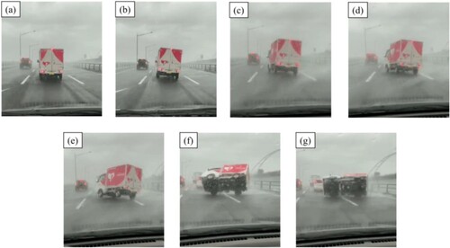
Vehicle stability when exposed to crosswind is one of the priorities in bridge design, particularly for vehicles with high-sided or lightweight features (Baker & Reynolds, 1992; Cheung & Chan, 2010). Figure 1 demonstrates a wind-induced accident of a van on a long-span bridge in Japan. It experienced lateral deviation ((a) ∼ (d)) and rollover ((e) ∼ (g)) during the accident. The aerodynamic performance of traveling vehicles is greatly influenced by the configuration of the bridge section (Alonso-Estébanez et al., 2018; Suzuki et al., 2003). Nevertheless, the development of bridge engineering has promoted the employment of rail-cum-road bridges, whose bridge section is more complicated than traditional long-span bridges. Among them, the single-level rail-cum-road bridge is a new form (Wang & Saul, 2020). It accommodates highway and railway on the same level. Thus, including the unknown and complex wind environment on the bridge deck, the train-induced wind would exert additional threaten on the highway vehicles.

Figure 1. Wind-induced accident in Japan.

Nowadays, researches about the aerodynamic performance of vehicles on bridges mainly rely on wind tunnel test and CFD techniques. Static models are usually used since the actual traveling condition could be equally researched through the relative velocity method (Han et al., 2019; Zhu et al., 2012). Based on a series of wind tunnel tests, Zhu et al. (2012) measured the aerodynamic forces and moments of four types of road vehicles on the ground and a typical box girder. The aerodynamic characteristics of vehicles have been analyzed, and the results provide a valuable reference for practical engineering. With a 1:40 scale wind-tunnel model, Dorigatti et al. (2012) explored the aerodynamic loads of three road vehicles with a high-sided feature on an ideal deck and a typical box girder. The aerodynamic characteristics of these vehicles under different wind directions are comprehensively compared. To investigated the cause of two consecutive wind-induced accidents on a double-deck highway bridge in South Korea, Kim et al. (2020) performed a 1:70 wind-tunnel testing. The experiment reveals that the net distance between the upper and lower decks is an influential factor for vehicle vulnerability. The CFD method has developed quickly in recent years (Ghalandari et al., 2019; Salih et al., 2019). With CFD technology, Wang et al. (2013) simulated the aerodynamic forces on a vehicle-bridge deck system through the large-eddy simulation (LES) method. The numerical model was compared with the wind tunnel test, and the traveling condition was researched through a relative velocity method. Based on numerical simulation, Alonso-Estébanez et al. (2018) particularized the aerodynamic forces of a bus on several classes of bridge decks, the parameters concerning the bridge configuration are thoroughly investigated. The results indicate that the box bridge deck's only geometry parameter that significantly influences bus aerodynamics is the box height.

Moreover, it has been verified that the gust load of moving trains shows a significant influence on surrounding infrastructures such as stations (Zhou et al., 2014), bridges (Yang et al., 2015; Yao et al., 2020), wind barriers (Tokunaga et al., 2016; Xiong et al., 2018; Zou et al., 2019), etc. However, the influence of train-induced wind on road vehicles is a new issue. Existing researches are primarily about the aerodynamic interference between two trains, and the rapid development of computer technologies and algorithms has popularized the CFD techniques. Sun et al. (2014) investigated the aerodynamics of two train meeting in the open air and the tunnel through moving grid techniques. The safety issue is discussed with a multi-body system. During the encounter, strong fluctuation of drag and lateral forces were observed. Chen and Wu (2018) researched the aerodynamic performance of two trains meeting in the open air with the finite volume method. The results show that the damage of the lateral window glass derives from the suction of negative pressure. Li et al. (2020) researched the aerodynamic issue of two trains crossing each other in a tunnel through a validated numerical model. The characteristics of the components of the slipstream were fully reported at different spatial positions. Huang et al. (2019) introduced an unsteady model on the aerodynamic issue of two meeting high-speed maglev trains. The transient pressure on train surfaces as well as the slipstream distribution on the trackside is analyzed. The research suggested a 6 m of safe trackside distance if considering the condition of maglev trains passing each other at the speed of 430 km/h.

As reviewed above, a vast complex deck and the aerodynamic impact of train-induced wind are the potential unfavorable factors influencing traveling safety. Both of them are newly generated with the employment of the single-level rail-cum-road bridge. Since relevant research is sparse, this paper aims to help understand the adverse wind environment on a single-level rail-cum-road bridge and provide quantitative analysis. With this aim in mind, the following objectives are arranged:

• Obtain the variation feature of the flow field on the vehicle-bridge system under the combination of crosswind and train-induced wind, utilize corresponding results to explain the impact mechanism.

• Quantitatively analyze the dilemma that vehicles on an upstream lane are burdened with more significant static wind load while the aerodynamic impact from the moving trains is slighter.

• Investigate how the crosswind and train-induced wind influence high-sided road vehicles with different geometrical configurations.

• Explore how the crosswind affects the effect of the train-induced wind on the road vehicle, find a quick and conservative way that could obtain the aerodynamic forces of road vehicles under crosswind and train-induced wind through several CFD cases.

To achieve these objectives, a 3D CFD numerical model was carried out to simulate the aerodynamic loads of high-sided road vehicles on a single-level rail-cum-road bridge under crosswind and train-induced wind. Due to the complex wind environment, the main challenge in the present study is improving the accuracy of the numerical model and conducting corresponding validations. To overcome this, four aspects of the numerical accuracy are discussed. A large-scale wind tunnel sectional model test was conducted and compared with the numerical model to validate the capability of the numerical model on simulating the wind environment of the researched single-level rail-cum-road bridge. A moving model test was carried out on the availability of the achievement of dynamic mesh as well as the feasibility of the simplification of bridge deck system; the results of traveling conditions are also compared with previous researches (Kim et al., 2020; Zhu et al., 2012) to show the reasonability.

Section 2 describes the details of the numerical model. Then, in section 3, the numerical model is verified in grid independence, calculation domain, grid resolution and dynamic mesh technique. In section 4, the research objectives are thoroughly conducted. In the last section, the main conclusions of this study are explained.

2. CFD numerical model

2.1. Geometrical model

2.1.1. Bridge model

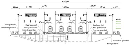
The Yibin Lingang Yangtze River Bridge, a single-level rail-cum-road bridge under construction and located over the Yangtze River in Yibin, China, is introduced in the present research (Wang & Saul, 2020). The span arrangement is 72.5m+203m+522m+203m+72.5 m.The main girder is 63.9 m in width and 5 m in height, and the distribution of the bridge deck system is illustrated in Figure 2. The cross-section is characterized by four railway lines in the middle and three highway lanes on both sides. To cite the vehicle location conveniently, all railway lines and highway lanes are numbered according to the direction of the upcoming flow. When transformed into the numerical model, the geometrical feature of the main girder is kept, while to enhance the simulation efficiency, the bridge deck system is simplified. Components such as vertical columns are omitted, the guardrails and barriers are simplified to rods with the principle of equivalent ventilation ratio and thickness. All the windward bridge deck system is kept in the verification cases, nevertheless, since the deck system greatly increases the grid number, thus, for traveling cases, only the concrete wall and anti-glare barrier are considered in the simulation of moving cases.

Figure 2. Cross-section of Yibin Lingang Yangtze River Bridge (Unit: mm) (Wang & Saul, 2020).

2.1.2. Vehicle model

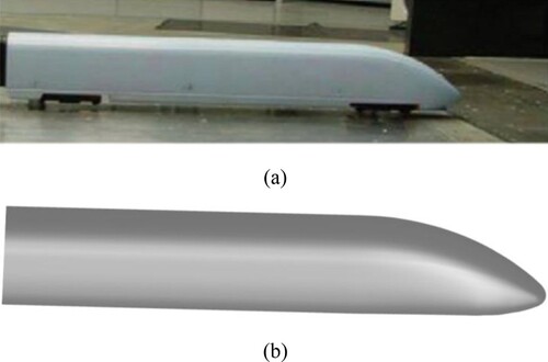
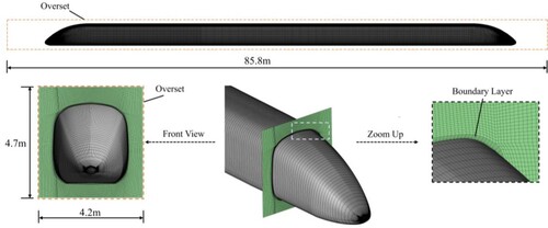
The CRH3 EMU is employed in the present study. It is the designed vehicle type of Yibin Lingang Yangtze River Bridge and is widely adopted in Chinese railway transportation (Xiang et al., 2015; Yang et al., 2019). Previous study has shown that the aerodynamic impact from the moving train is mainly derived from the fierce airflow around the train’s nose and tail (Chen & Wu, 2018; Huang et al., 2019; Sun et al., 2014). To thoroughly research the aerodynamic impact of trains, three carriages are included in the formation of the trains, i.e. the head carriage, the middle carriage and the tail carriage. The train formation is also adopted in some other studies (Liu et al., 2018; Niu et al., 2018). The length of the head carriage and tail carriage is 24.6 m and the middle carriage is 24.8 m. The height and width of the typical section are 3.45 and 3.25 m, respectively. To improve the mesh quality and accelerates the numerical simulation, the substructure of the train is simplified. At the same time, the critical features of the train body that affect its aerodynamic performance are kept. The appearance of the CRH3 model and its scaled prototype is shown in Figure 3.

Figure 3. The configuration of the CRH3 model: (a) Scaled prototype from Schober et al. (2010); (b) Numerical model in the present study.

As for road vehicles, the high-sided road vehicles have a larger windshield area, so they are more accessible to sideslip and roll over under strong wind conditions (Baker, 1988). Similarly, it could be inferred that the influence of train-induced wind is more threatening for high-sided road vehicles. Three kinds of high-sided road vehicles are introduced for the research: a van, a bus, and a truck trailer. These vehicles are also applied in the research of the aerodynamic performance of the vehicle-bridge system of the Pingtan rail-cum-road bridge (Chen et al., 2015). The configurations of the road vehicles are shown in Figure 4, the definition of the five-component force is appended in Figure 4 (c), relevant dimensional information is given in Table 1.

Figure 4. Configuration of the road vehicle: (a) Van; (b) Bus; (c) Truck trailer.

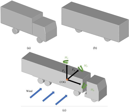
Table 1. Geometrical information about the road vehicles.

	Length	Width	Height	COG from the	COG above the
	(m)	(m)	(m)	head (m)	ground (m)
Van	7.67	2.3	3.34	3.84	1.55
Bus	10.42	2.5	3.29	5.64	1.495
Truck trailer	15.72	2.48	3.78	6.30	1.62

*Note: COG – center of gravity

2.2. Calculation domain and mesh generation

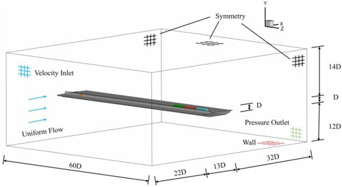
The geometrical detail of the calculation domain adopted in the simulation is shown in Figure 5 (D is the height of the main girder without considering the deck system), and the boundary condition is shown accordingly. Considering the large size of the bridge deck, the length of the calculation domain (length in the x direction) should be large enough to eliminate the influence from the domain boundary. Nevertheless, an oversize calculation domain would generate redundant mesh cells and decrease the simulation efficiency. With the help of trial calculation, the dimension of the calculation domain is determined. The blocking ratio is about 3.7% and could meet the 5% requirement in numerical wind tunnel simulation.

Figure 5. Calculation domain and boundary condition.

The calculation domain is divided into three zones for mesh generation, i.e. the bridge zone, the road vehicle zone and the train zone. For the simplified bridge model, the structural hexahedral grid is adopted. However, due to the sizeable dimensional difference between the deck system and the main girder, it is hard to produce grids with enough resolution near the wall boundary with this strategy. To solve this, an enhanced non-structural zone near the bridge deck system was generated. In terms of the train zone, it only contains structural hexahedral cells. For the road vehicle zone, prism cells are firstly generated near the vehicle surface. Then tetrahedral cells are introduced to fill the rest of the space. It is noted that the overset mesh achieves the motion of vehicles in the dynamic mesh module. It would easily produce ‘orphan cells’ on the interface between the structured hexahedral grids and tetrahedral grids. Additional structural hexahedral grids are employed outside the tetrahedral grids to maintain a similar grid resolution between the bridge and road vehicle zones The trial case showed that the mentioned processing had removed 1624 ‘orphan cells’ near the overset boundary of the van.

Moreover, boundary layers are generated near the wall boundary to enhance the simulation of the shear flow. The height of the first layer of the bridge is 10 mm, and the height of the first layer of the deck system is 3 mm. The height of the first layer of the road vehicle is 5 mm with an expansion ratio of 1.1, it has eight layers in total, and the trial case showed the y+ range was 130 ∼ 160; the height of the first layer of the train is 3 mm with an expansion ratio of 1.1, it has eight layers in total, and the trial case showed the y+ range was 170 ∼ 210, which is similar with Yang et al. (2019). The grids around the domain and the bridge deck are shown in Figure 6. The grids in the road vehicle zone are shown in Figure 7, and the grids in the train zone are shown in Figure 8.

Figure 6. Structural and non-structural hexahedral gird area: (a) calculation domain; (b) bridge deck.

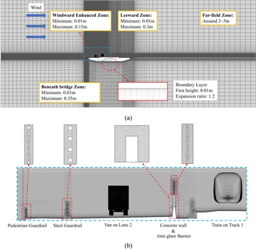
Figure 7. Mesh generation and boundary condition of road vehicle zone (Van).

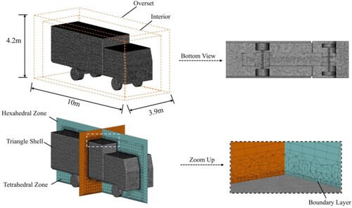
Figure 8. Mesh generation and boundary condition of train zone.

2.3. Turbulence model and solution parameters

In the simulation, the air is considered incompressible since the train speed is 300 km/h and the discussed wind speed is less than 25 m/s, the Mach number Ma = U_r/a =  ≈ 0.25 < 0.3 accordingly. Where U_r is the resultant wind velocity, U_w is the wind speed, U_v is the vehicle speed, a is the local sound velocity.

The flow around the vehicle-bridge system is highly turbulent. Scale-Resolving Simulation (SRS) models such as Large Eddy Simulation (LES) are theoretically more suitable chosen as the turbulence model. However, it requires grids with a very high resolution close to the wall as well as a relatively small solution step. The calculation resources and time are unaffordable because the single-level rail-cum-road section has a giant dimensional configuration and complex bridge deck system. As an alternative, the Reynold averaged Navier-Stokes (RANS) model could offer the most economical approach for computing complicated turbulent industrial flows.

The simulation accuracy of the RANS model highly depends on the turbulence model. Among the turbulence models, the shear-stress transport (SST) $k-\omega$ model (Menter et al., 2003) introduced turbulent viscosity formulation to consider the transport effects of the principal turbulent shear stress. It became popular in simulations on moving high-speed trains (Liang et al., 2020; Yao et al., 2020; Zou et al., 2020) and was adopted in the turbulence simulation. The turbulence kinetic energy k, and the specific dissipation rate $\omega$, can be obtained by additional equations: (1) $\begin{array}{rl}\frac{\mathrm{\partial }}{\mathrm{\partial }t}\left(\rho k\right)+\frac{\mathrm{\partial }}{\mathrm{\partial }{x}_i}\left(\rho k{u}_i\right)& =\frac{\mathrm{\partial }}{\mathrm{\partial }{x}_j}\left({\mathrm{\Gamma }}_k\frac{\mathrm{\partial }k}{\mathrm{\partial }{x}_j}\right)+G_k-Y_k+S_k\end{array}$(1) (2) $\begin{array}{rl}\frac{\mathrm{\partial }}{\mathrm{\partial }t}\left(\rho \omega \right)+\frac{\mathrm{\partial }}{\mathrm{\partial }{x}_i}\left(\rho \omega u_i\right)& =\frac{\mathrm{\partial }}{\mathrm{\partial }{x}_j}\left({\mathrm{\Gamma }}_{\omega }\frac{\mathrm{\partial }\omega }{\mathrm{\partial }{x}_j}\right)+G_{\omega }-Y_{\omega }+S_{\omega }\end{array}$(2) Where, $G_k$ and $G_{\omega }$ are the generation of turbulence kinetic energy and dissipation rate derived by mean velocity gradients, respectively. ${\mathrm{\Gamma }}_k$ and ${\mathrm{\Gamma }}_{\omega }$ represent the effective diffusivity of k and $\omega$, respectively. Y_k and $Y_{\omega }$ are the dissipation of k and $\omega$ because of turbulence. $S_k$ and $S_{\omega }$ are user-defined source terms.

The coupled algorithm is adopted due to the compatibility of overset dynamic mesh technique. The second-order upwind format is introduced to discretize the momentum continuity, turbulent kinetic energy and dissipation rate. The trial cases suggest a time step of 0.003s, and the Courant number is generally smaller than 2. The convergence condition is set to be 10⁻⁴ for all the monitored values. The maximum iteration step is 30 in each time step, and the total time step is about 1200.

2.4. Overset mesh technique

There are several ways of simulating moving objects, such as smoothing, layering, remeshing and overset (Jasak, 2009). Among them, the overset mesh technique is easier for mesh generation, more flexible in dynamic grid processing, and has less fluctuation in the mesh quality during updating the computational domain (Prewitt et al., 2000). Thus, it becomes popular to research the aerodynamic performance of moving vehicles recently. (Broniszewski & Piechna, 2019; Wang et al., 2021; Yao et al., 2020).

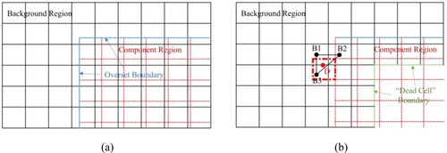
The separated generation characterizes the overset mesh technique on the mesh of ‘Background Region’ and ‘Component Region’. The ‘Background Region’ provides the essential feature of the flow field of the terrain, and the ‘Component Region’ receives the transported data and further computes the flow field inside. It requires similar mesh resolution around the ‘Component Region’, but there is no connectivity. Shell meshes on their interfaces are non-formal. To form available meshes for computation, it introduces assembly and interpolation strategies in the overset technique.

Figure 9 shows the mesh updating workflow in a single time step. Figure 9 (a) demonstrates the initial meshes before the solution. Meshes with black lines belong to the ‘Background Region’, meshes with red dotted lines belong to the ‘Component Region’. The boundary with blue lines is identified as the overset interface. According to their relative location, all the meshes are divided into three kinds of mesh, ‘dead cells’ that won’t participate in the calculation, ‘receptor cells’ which are overlapped on the ‘Background Region’, and ‘solve cells’ contribute to the solution. As the assembly starts, the ‘dead cells’ are first identified and excluded from the solving process, such as the disappeared cell in the ‘Background Region’ in Figure 9 (b). Then ‘donor cells’, which are part of the receptor cells located between the two regions, are identified, such as the red thick dotted box in (b). The assembly process finishes, and the interpolation strategy is adopted to achieve connectivity between the two regions. As shown in Figure 9 (b), once a ‘doner cell’ D is identified, three adjacent cells B1, B2 and B3 in ‘Background Region’ provide dates for the interpolation.

Figure 9. Flow chart of overset mesh: (a) Assembly; (b) Interpolation.

3. Model verification

3.1. Grid independence

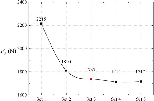
Five sets of grids, including the preceding one, are taken for the verification of grid independence. The grid number of the five sets of grids is given in Table 2, the main difference among the grids lies in the minimum and maximum cell size around the windward road lanes and vehicle overset regions and the parameters of the boundary layers around the car and train.

Table 2. Grid information in the grid independence verification (Unit: million).

	Bridge region	Van region	Train region	Total
Set 1	5.4	Non-struct: 0.71 Struct: 0.009	1.16	7.28
Set 2	7.7	Non-struct: 1.13 Struct: 0.014	1.98	10.82
Set 3	9.5	Non-struct: 1.22 Struct: 0.017	2.44	13.18
Set 4 (Adopted in present study)	10.9	Non-struct: 1.47 Struct: 0.020	2.81	15.20
Set 5	14.1	Non-struct: 1.83 Struct: 0.025	3.31	19.27

The side force F_S of the van on lane 3 is extracted for comparison, and the steady results are shown in Figure 10. According to Figure 10, it could be seen that the side force of the van on lane 3 decreases as the grid number increases, a relatively sharp drop is observed when it moves from Set 1 to Set 3, and a slight drop occurs when it moves from Set 3 to Set 4. Nevertheless, the results of Set 4 and Set 5 are close, and Set 5 even produces a slightly larger result. It could be concluded that the resolution of Set 4 is enough to capture the major flow characteristics around the windward lanes and the vehicles, so the grids of Set 4 are employed in the following calculation.

Figure 10. Fs of the van on lane 3 in different mesh resolution.

3.2. Parameters of the calculation domain

In comparison with studies concerning the aerodynamic performance of vehicles on bridges (Alonso-Estébanez et al., 2017; Han et al., 2018; Zhou & Zhu, 2020), the scale of the calculation domain adopted in the present research is comparatively small. The small calculation domain is ascribed to the large scale of the bridge model and the purpose of balancing the computational efficiency of dynamic mesh. Hence, the dimensional configuration of the calculation domain was investigated to show whether the boundary affects the flow field around the bridge model. The steady calculation was conducted when there is only the bridge model in the domain. The velocity contour around the domain at the wind speed of 15 m/s is demonstrated in Figure 11.

Figure 11. Velocity contour of the steady computation.

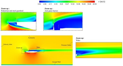
According to Figure 11, it is noted that the boundaries of the calculation domain have limited influence on the flow field around the bridge deck. The upcoming wind derived from the velocity inlet has fully developed before arriving at the bridge. The major development of the wake effect of the bridge has been captured in the given distance. As for the vertical distance, there is enough space between the bottom of the bridge and the ground wall, so the shear flow layer near the ground has little effect on the bridge. Meanwhile, the upper symmetry is also far enough from the bridge to completely capture the block effect near the windward deck. In addition, according to the local contour of the bridge deck system, the given resolution of the grids around the bridge deck system could provide a clear view of the flow detail. It is noted that due to its small geometrical feature and high ventilation, the pedestrian guardrail and anti-glare barrier have a limited shelter effect on the upcoming wind. However, noticeable disruption in the wind due to the steel guardrail and concrete wall is observed.

3.3. Static aerodynamic force on the bridge deck

3.3.1. Experiment parameters

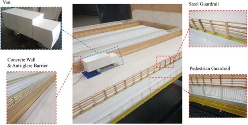
The large-scale sectional model wind tunnel test was conducted in the XNJD-3 wind tunnel laboratory in Southwest Jiaotong University. The length, width and height of the wind tunnel is 36.0, 22.5 and 4.5 m, respectively. The wind speed could vary from 0 ∼ 16.5 m/s and the turbulence I_z is under 1.5%. The scale ratio is 1:20 to achieve a relatively large Reynold number and preserve the details of the bridge deck system. The length of the sectional model is 3.9 m, the blockage ratio is about 1%. Details of the test are given in Figure 12.

Figure 12. Large-scale sectional model wind tunnel test.

The aerodynamic forces of road vehicles are measured by the KWR46A force balance, which has a force range of ±50 N and a moment range of ±50 N·m. The sampling frequency is 1 kHz, and the sampling time is over 15 s in each measurement. The acquired forces are transferred into five-component aerodynamic coefficients through equation (3(3) $\begin{array}{rl}{C}_{\text{S}}& =\frac{F_{\text{S}}}{\text{q}{A}_f},C_{\text{L}}=\frac{F_{\text{L}}}{\text{q}{A}_f},C_{\text{MR}}=\frac{M_{\text{R}}}{\text{q}{A}_f{h}_v},\\ C_{\text{MY}}& =\frac{M_{\text{Y}}}{\text{q}{A}_f{h}_v},C_{\text{MP}}=\frac{M_{\text{P}}}{\text{q}{A}_f{h}_v}\end{array}$(3) ): (3) $\begin{array}{rl}{C}_{\text{S}}& =\frac{F_{\text{S}}}{\text{q}{A}_f},C_{\text{L}}=\frac{F_{\text{L}}}{\text{q}{A}_f},C_{\text{MR}}=\frac{M_{\text{R}}}{\text{q}{A}_f{h}_v},\\ C_{\text{MY}}& =\frac{M_{\text{Y}}}{\text{q}{A}_f{h}_v},C_{\text{MP}}=\frac{M_{\text{P}}}{\text{q}{A}_f{h}_v}\end{array}$(3) Where C_S, C_L, C_MR, C_MY, C_MP are side force coefficient, lift force coefficient, rolling moment coefficient, yawing moment coefficient and pitching moment coefficient, respectively; F_S, F_L, M_R, M_Y, M_P are side force, lift force, rolling moment, yawing moment and pitching moment acing on the road vehicle; A_f is the reference aera which represent the side area of the vehicle flank, h_v is the height of the COG of the vehicle; $q=0.5\rho U_r^2$, $\rho$ is the air density and U_r is the resultant wind speed.

The CFD model also has a scale ratio of 1:20, the wind speed of the CFD model and experiment are both 10 m/s, and the Reynolds number (based on the wind speed and the height of the vehicle model) is about 8.81×10⁴ in the experiment and CFD model. The yaw angle of the CFD model and experiment are both 90°.

3.3.2. Results comparison

The aerodynamic coefficients of the van on three windward lanes are compared and shown in Table 3, the percentage error e is calculated by equation (4(4) $e=\frac{C_{\text{sim}}-C_{exp}}{C_{exp}}\times 100\mathrm{\%}$(4) ): (4) $e=\frac{C_{\text{sim}}-C_{exp}}{C_{exp}}\times 100\mathrm{\%}$(4) Where C_sim and C_exp are the aerodynamic coefficients in simulation and experiment, respectively.

Table 3. Comparison between the wind tunnel test and simulation.

Lane Location		CS	CL	CMR	CMY	CMP
Lane 1	Exp	1.575	0.576	−0.016	−0.776	0.108
	Sim	1.458	0.465	−0.173	−0.689	−0.089
	e (%)	−7.43	−19.17	958.33	−11.22	−182.66
Lane 2	Exp	0.842	−0.106	−0.102	−0.375	0.172
	Sim	0.741	−0.074	−0.159	−0.400	0.102
	e (%)	−12.01	−29.57	56.00	6.91	−40.48
Lane 3	Exp	0.468	−0.162	−0.131	−0.315	0.163
	Sim	0.448	−0.128	−0.078	−0.308	0.114
	e (%)	−4.26	−21.47	−40.63	−2.16	−30.00

*Note: Exp - Experiment, Sim - Simulation

According to Table 3, it could be seen that the simulation results match well with the results of the experiment. For the C_s and C_MY, the maximum percentage error is about 12%, and the minimum percentage error is within 3%. In terms of C_MR, it is possibly due to the simplification of the bridge model that the percentage error is relatively large. However, both results possess a small absolute value, and the absolute difference is also slight. As for the C_L and C_MP, both aerodynamic coefficients possess small values on different lanes despite the large percentage error between the simulation and experiment. The absolute differences are also minor, the simulation on these two aerodynamic coefficients is considered reasonable. In general, the simulation is considered accurate enough in terms of the C_S, C_MR and C_MY that mainly determines the vehicle response and handling (Salati et al., 2019, 2018).

3.4. Aerodynamic load of moving vehicle

Moving model tests were carried out to further validate the achievement of dynamic mesh and the simulation of the anti-glare barrier. Both the CFD model and the experiment have a scale ratio of 1:20, and the Reynolds number (based on the train speed and the height of the train model) is about 9.16×10⁴ in the experiment and CFD model. The yaw angle of the CFD model and experiment are both 0°.

3.4.1. Experiment parameters

A dynamic system is applied to achieve the motion of the vehicle model, which is composed of a wide bridge deck, several holders, wind barriers, a linear module and a serve motor (Xiang et al., 2017). The sliding plate is where the vehicle model is installed, and the sliding plate was connected to the servo motor by a synchronous belt. Thus, the whole system is activated by the servo motor. The whole dynamic system is shown in Figure 13.

Figure 13. Moving model system and test condition: (a) Vertical view; (b) Side view.

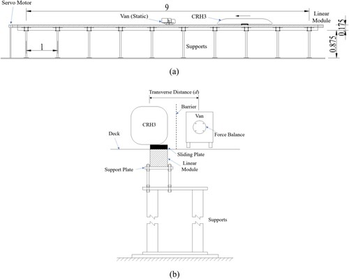
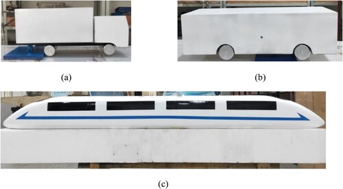
Four kinds of vehicles are included in this moving model tests for different verification purposes. The van and the CRH3 train are applied in Section 3.4.2, the bus and the cuboid train are applied in Section 3.4.3. The features of the vehicles are the same as the ones in Section 2.1.2. Nevertheless, given the limited length of the guide rail, the length of the CRH3 train is shortened, which is 1.75 m in total (35 m in prototype). The cuboid train possesses the same length, width and height as the CRH3 train. The corresponding vehicles are shown in Figure 14. The aerodynamic load on the van was measured by the KWR46-A force balance too.

Figure 14. Vehicle models in the moving model tests: (a) Van; (b) Bus; (c) CRH3 (up) and cuboid train (down).

3.4.2. Aerodynamic load of train-induced wind

The van and CRH3 train were used to verify the aerodynamic impact of the streamlined train on a road vehicle with a comparatively complicated configuration. Since the dynamic system could only realize the movement of a single vehicle, the case when the van was static and the train passed by was selected for comparison. The transverse distance between the two vehicles was set as 0.22 m (4.4 m in prototype).

In this test, the speed of the train in the uniform stage is 7 m/s. To be consistent with the moving model test, the CFD model employed in this comparison shares the same parameters as described in Section 2.2 ∼ 2.3, and the overset mesh technique is applied to the motion of the train. The trial tests showed that only the side force of the van got apparent fluctuation when the train passed. Therefore, the time history of the equivalent side force coefficient, which is defined in equation (5(5) $C_{\text{S}}=\frac{F_{\text{S}}}{\frac{1}{2}\rho {V_{\text{t}}}^{2}HL}$(5) ), is extracted for comparison. (5) $C_{\text{S}}=\frac{F_{\text{S}}}{\frac{1}{2}\rho {V_{\text{t}}}^{2}HL}$(5) Where F_S is the side force on the van, $\rho$ is the air density, V_t is the train speed, L and H are the length and the height of the van, respectively.

The comparison of C_S is illustrated in Figure 15. According to Figure 15, it could be seen that the variation trend of the experiment and the simulation are highly parallel. Both of them possess three peak values P1 ∼ P3, and two valley values V1 ∼ V2. The variation from P1-V1 and V2-P3 are similar, while the primary difference locates at the curves of V1-V2. The variation of the experiment curve is more intense, which may be ascribed to the vibration of the experiment system. The specific values of peaks and valleys are extracted for further discussion, which is shown in Table 4. From Table 4, it could be seen that the percentage errors are within a reasonable range. The percentage error of the five discussed values is around 5%. The maximum error is 6.20% for P2, and the minimum error is −1.24% for V2.

Figure 15. Comparison of the variation curve of C_S.

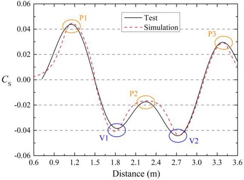
Table 4. Quantitative comparisons among the peak/valleyvalues.

	P1	V1	P2	V2	P3
Experiment	0.04377	−0.03850	−0.01743	−0.04426	0.02961
Simulation	0.04465	−0.04022	−0.01635	−0.04371	0.02891
Percentage Error (%)	2.01	4.47	−6.20	−1.24	−2.36

3.4.3. Simulation of anti-glare barrier

The anti-glare barrier is simplified into rods in the numerical model by the principle of equivalent ventilation rate. An accurate simulation of such windshield effect is required to recover the actual condition.

The measured force is influenced by the vibration of the test system. As can be seen in Section 3.4.2, the measured force is small, and it will be smaller when the anti-glare barrier is installed. Thus, the vibration of the test system will have a larger influence on the results when the anti-glare barrier is installed. It could be deduced that the additional force produced by the vibration of the test system is relatively fix, so as long as the force on the test vehicle increases, the proportion of the force produced by the vibration of the test system will be smaller, the test error hence will be smaller. Through comparing the combinations of road vehicle and train, we found that the measured force is the largest when a cuboid train passing by the bus, so the bus and cuboid train were selected in the verification of the simulation of anti-glare barrier. The height of the anti-glare barrier is 17.5 cm (3.5 m in prototype), with a ventilation rate of 60%. The parameters in the numerical model refer to the one in Section 2.2.

The peak value P1 and valley value V1 of C_S are extracted for comparison to verify the attenuation effect on the push and suction. The results at the transverse distance of 22, 26 and 30 cm (4.4, 5.2, 6 m in prototype) are compared and shown in Figure 16. The comparison of the attenuation ratio defined in equation (6(6) $\xi \text{ = }\frac{C_{\text{S - AGB}}}{C_{\text{S - Initial}}}$(6) ) is shown accordingly. (6) $\xi \text{ = }\frac{C_{\text{S - AGB}}}{C_{\text{S - Initial}}}$(6) Where C_S-AGB is the side force coefficient with the anti-glare barrier, C_S-Initial is the side force coefficient without the anti-glare barrier.

Figure 16. Comparison of peak/valley values and attenuation ratio: (a) P1; (b) V1.

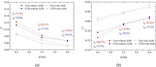
According to Figure 16, it could be seen that the results of the numerical model are highly consistent with the ones of the moving model test. The test and numerical model have similar peak values and valley values in all the cases. For P1, the attenuation ratio of the test is about 70% ∼ 80%, while that of the simulation is about 75%. For V1, the attenuation ratio of the test is about 60% ∼ 75%, while that of the simulation is about 70%. In different cases, the attenuation ratios of the numerical model are comparatively stable, but that of the moving model test have apparent differences, which is possibly ascribed to the vibration of the test system. The maximum difference is at the V1 of the third case, the attenuation ratio of the test is 61.8%, and that of the simulation is 72.3%.

4. Results and analysis

In the following cases, road vehicle and train travel toward each other. The speed of the road vehicle is 80 km/h and the speed of the train is 300 km/h.

4.1. Flow features

First of all, the flow features of the vehicle-bridge system are studied through CFD visualization technology. Figure 17 shows the pressure distribution around the sole-traveling vehicles included the van and the train.

Figure 17. Pressure distribution of sole-traveling vehicle: (a1) ∼ (a2) Pressure iso-value surface of 100 Pa; (b1) ∼ (b2) Pressure distribution on the vehicle-bridge system; (c1) ∼ (c2) Horizontal plane 1.5 m above the deck. (Unit: Pa).

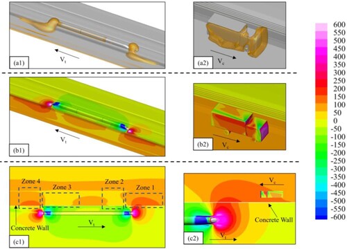
According to Figure 17 (a1), it could be seen that the spatial pressure distribution near the nose and tail of the traveling train is blocked and stretched by the concrete wall. The spherical iso-surface near the train nose and tail moves across the concrete wall and gets superposed with the crosswind, generating a narrow area with high pressure. According to Figure 17 (b1), the pressure wave derived from the moving train significantly changes the pressure distribution on the bridge deck, making the pressure near the train nose and train tail higher and the pressure near the middle carriage is lower. A similar phenomenon could be observed in the horizontal plane 1.5 m above the bridge deck (Figure 17 (c1)). The pressure distribution around the moving train could be divided into four areas denoted by Zone 1 ∼ Zone 4 and a transition. Zone 1 ∼ Zone 4 are considered the leading cause of the aerodynamic variations of the meeting road vehicle.

In contrast, the traveling van has limited influence on its nearby structures. As shown in Figure 17 (a2), the pressure iso-surface of 100 Pa envelopes the van’s body, and Figure 17 (b2) also indicates that the van’s motion has not influenced the nearby bridge deck. There is little upstream bridge deck system for the highway, and the location is more upstream than the railway, so the superposition of vehicle-induced wind and crosswind is more pronounced. The pressure distribution on the vehicle body is nonsymmetrical, and the high-pressure zone locates at the right rear of the vehicle body. Moreover, according to Figure 17 (c2), when the van travels into the influencing zone of the train, it still has little effect on the surrounding pressure distribution.

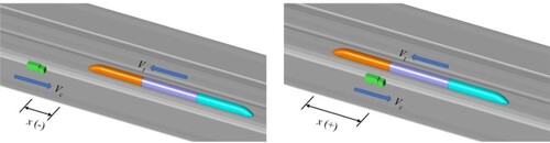
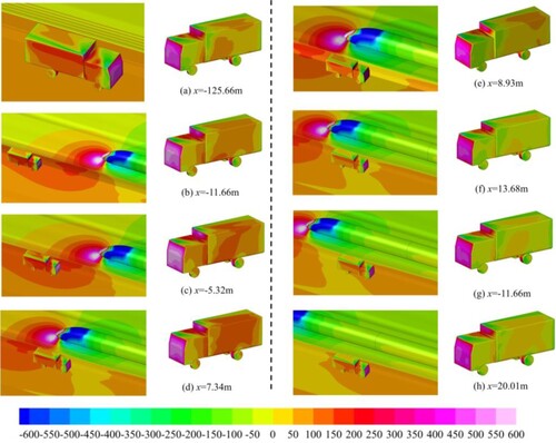
To give an in-depth investigation on the impact mechanism of the train-induced wind, Figure 19 demonstrates the pressure distribution on the van’s body when traveling near the head carriage. As shown in Figure 17, the effect of the train nose and train tail on the vehicle-bridge system is similar. To be concise, only the process when the van traveling near the head carriage is discussed. For each subfigure, the left picture shows the pressure distribution of the vehicle-bridge system, and the right one supplements the pressure distribution of the van’s leeward flank. The net distance in their moving direction (x) is defined to show the vehicles’ relative location (seen in Figure 18). Before the encounter, x is with a negative value. After the vehicles’ heads meet each other, x is with a positive value.

Figure 18. Definition of the relative location.

It could be seen in Figure 19 (a) that the crosswind and the van’s vehicle-wind bring a high-pressure zone on the windward flank of the van, the area with the highest pressure locates at the upper flange. For the leeward side, prominent high-pressure zones exist at the left bottom and the upper right of the carriage. As the van gets close to the train (Figure 19 (b)), the high-pressure area expands, the high-pressure zone on the windward flank spreads downward, while the ones on the leeward flank spread upward right and generate the highest-pressure zone at the left bottom. As the vehicles move on (Figure 19 (c)), the high-pressure zone at the left bottom expands toward the upper right, bringing a sizeable high-pressure area on the leeward flank (Figure 19 (d)). Then the van moves into Zone 2 (Figure 19 (e)), the high-pressure zone leaves the vehicle body from the upper right. At this time, a low-pressure zone occurs at the left bottom of the leeward flank. The low-pressure zone gradually fills the leeward flank (Figure 19 (f)) as the van leaves the scope of influence of the head carriage (Figure 19 (g)), then the pressure on the leeward flank increases and stays stable (Figure 19 (h)), while it is still lower than the one of sole-traveling state (Figure 19 (a)). During the process, the pressure variation on the windward flank is not significant.

Figure 19. Pressure distribution on the vehicle-bridge system (Unit: Pa).

Two points are noteworthy during the process:

Point 1: For the pressure increase and decrease on the leeward flank, the variation starts from the left bottom and gradually fills the whole carriage, then leaves the van body from the upper right.

Point 2: The variation from the high-pressure zone to the low-pressure zone is continuous, so there exist moments when both of them exert on the leeward flank.

4.2. Effect of train-induced wind on different lanes

For traditional long-span bridges, the traveling condition is safer on a downstream lane. As for the three windward lanes on the single-level rail-cum-road bridge, the transverse distance to the train is smaller when the road vehicle travels on a downstream lane. The road vehicle would experience a fiercer fluctuation as the train passes by. The case details are given in Table 5, the aerodynamic coefficients calculated by equation (3(3) $\begin{array}{rl}{C}_{\text{S}}& =\frac{F_{\text{S}}}{\text{q}{A}_f},C_{\text{L}}=\frac{F_{\text{L}}}{\text{q}{A}_f},C_{\text{MR}}=\frac{M_{\text{R}}}{\text{q}{A}_f{h}_v},\\ C_{\text{MY}}& =\frac{M_{\text{Y}}}{\text{q}{A}_f{h}_v},C_{\text{MP}}=\frac{M_{\text{P}}}{\text{q}{A}_f{h}_v}\end{array}$(3) ) are illustrated in Figure 20. The horizontal dotted lines depict the sole-traveling state of the van, which are also represented by N_i (i  = 1, 2, 3, represents the case number). The vertical red dotted lines indicate the peak and valley values.

Figure 20. Aerodynamic coefficients of van on different lanes: (a) C_S; (b) C_L; (c) C_MR; (d) C_MY; (e) C_MP.

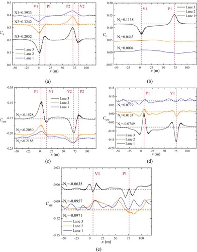
Table 5. Case details on different road lanes.

No. of	Location of	Location of	Speed	Wind Speed
Case	the Van	the Train	(km/h)	(m/s)
1	Lane 1	Track 1	Van: 80	15
2	Lane 2		Train: 300
3	Lane 3

According to Figure 20, it is noted that before the interference, the van traveling on an upstream lane has a larger value of C_S, which is consistent with the results in Section 3.3.2. The wind yaw angle is about 56°, and the C_S of case 1 ∼ 3 are 0.3933, 0.3242 and 0.2052, respectively. The difference with the results in Section 3.3.2 is possibly due to the removed windward deck system, which would increase the C_S, while a wind yaw angle of 56° would decrease it. As illustrated in Figure 11, the windward steel guard blocks the incoming flow and dramatically changes the downstream flow field, which may be why the C_L, C_MR and C_MY have different results from the ones in Section 3.3.2. In general, when all the coefficients are calculated through the resultant wind velocity, the values are all small, and the results are considered reasonable.

In terms of the effect of the train-induced wind, the variation process of all the aerodynamic coefficients could be divided into three stages: the meeting stage (x = −25 m ∼ 25 m), the plateau stage (x = 25 m ∼ 60 m) and the leaving stage (x = 60 m ∼ 110 m). These three stages indicate that the impact of the train-induced wind mainly originates from the head and the tail of the train, and the train body between them provide a relatively stable buffer zone. These features could also be referred from the pressure distribution near the trains (seen in Figure 17 (c1)). The variation trend of aerodynamic coefficients on different lanes also varies with the vehicle location. For the C_S and C_MR, both the meeting and leaving stages have two peak/valley values on lane 3. As it moves to lane 2 and lane 1, the second peak/valley value in the meeting stage and the leaving stage gradually disappear. The variation magnitude decreases as well, which is ascribed to the attenuation of the train-induced wind. The variation slope is less intense on an upstream lane, and the variation is distributed over longer distances. This phenomenon is because the iso-surface of the pressure contour around the train is like concentric circles (seen in Figure 17 (a1)). The further away from the train body, the pressure value is smaller, but the relevant iso-surface has a larger radius. Furthermore, it is noteworthy that the first peak/valley value in the meeting stage and leaving stage have comparable variation magnitude, e.g. for the C_S on lane 3, the difference value of N3 and V1 is close to the one of N3 and P2, so is the second peak/valley one. This phenomenon informs the impact from the head and tail of the train is similar in amplitude but reverse in direction.

For the C_L, there is only one peak/valley value in the meeting stage and the leaving stage on lane 3, while no noticeable fluctuation is observed on lane 1 and lane 2, which indicates that the vertical flow attenuates more rapidly compared to the horizontal flow. As for the C_MY and C_MP, the variation is more complicated. For C_MY on lane 3, three peak/valley values exist in the meeting and the leaving stage. This feature can be explained through Point 2 of Figure 19. Taking the meeting stage in C_MY as an example, it could be deduced that the first peak/valley value comes from Zone 1, the third peak/valley value comes from the Zone 2, and the second one derives from their superposition. The second one is large in amplitude because the suction of Zone 2 acts on the van’s tail and the push of Zone 1 acts on the van’s head, both of them produce a positive yawing moment.

Moreover, by comparing with the results of C_S, it could be seen that the peak/valley values of the C_S and C_MY do not coincide. For example, the V1 in C_S happens at x ≈ 3 m, while the V1 in C_MY happens at x ≈ −3 m, the time of the V1 in C_MY is before the one in C_S, which indicate that the peak/valley values do not cause the peak/valley values in C_MY in C_S. This phenomenon could explain why even the difference value between the V1 and P1 is large in C_S, the first peak/valley possesses a comparable value to the third one in C_MY. As it moves to lane 2 and lane 1, the fluctuation derived from train the are submerged in the oscillations derived from the crosswind. These oscillations are possibly due to the separating flow from the windward bridge deck. For the C_MP, this characteristic is more prominent, bringing a larger variation amplitude on lane 2 and lane 1.

Quantitative information about the variation amplitude, the normalized information with the results on lane 3, and the variation percentage compared to the aerodynamic coefficients before the interference (N_i) are summarized in Table 6. Since the meeting stage and the leaving stage have almost the same variations, only the values in the meeting stage are extracted. The C_S, C_MR and the C_MY, which mainly determine the traveling handling, are further discussed. For the C_S and C_MR, the variation amplitude is defined as the difference value between the V1 and P1; for the C_MY, it is the difference value between P1 and the adjacent valley value at x = −3 m.

Table 6. Quantitative information for the aerodynamic forces of the van on different lanes.

			Variation
Coefficients	Lane	Amplitude	Percentage (%)	Normalized
CS	Lane 1	0.0422	10.72	0.30
	Lane 2	0.0755	23.28	0.53
	Lane 3	0.1416	68.96	1.00
CMR	Lane 1	0.0242	11.09	0.34
	Lane 2	0.0312	15.21	0.44
	Lane 3	0.0705	46.10	1.00
CMY	Lane 1	0.0282	36.09	0.25
	Lane 2	0.0388	310.24	0.34
	Lane 3	0.1144	152.55	1.00

According to Table 6, it is noted that the train-induced wind changes the C_S and C_MR by about 10% for the van on lane 1, 20% for the van on lane 2 and 50% for the van on lane 3. The variation amplitudes of C_S, C_MR and C_MY on lane 2 and lane 1 are about 30% and 40% of those on lane 3, respectively.

4.3. Effect of train-induced wind on different vehicle type

To investigate the effect of train-induced wind on different vehicles. Three types of high-sided road vehicles are introduced in this section. The case details are shown in Table 7.

Table 7. Case details for the influence on different road vehicles.

No. of		Location of the	Location of	Speed	Wind Speed
Case	Vehicle Type	Road Vehicle	the Train	(km/h)	(m/s)
1	Van	Lane 3	Track 1	Road vehicle: 80	15
2	Bus			Train: 300
3	Truck Trailer

The comparison among the three types of vehicles is shown in Figure 21. The aerodynamic coefficients of the road vehicles before the aerodynamic impact are denoted by N_i (i = V - van, B - bus, T - truck trailer) and are listed accordingly.

Figure 21. Aerodynamic forces of different road vehicle: (a) C_S; (b) C_L; (c) C_MR; (d) C_MY; (e) C_MP.

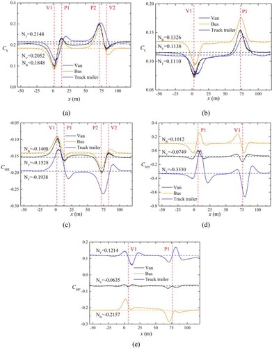
As shown in Figure 21, before the impact of train-induced wind, the aerodynamic forces are highly related to the vehicle’s geometrical feature. Due to their similar height, the C_S of the three cars is about 0.2, the C_L is about 0.1 ∼ 0.15, and the C_MR is about −0.1 ∼ −0.2. Nevertheless, the C_MY and C_MP of the three vehicles vary a lot because of the difference in the vehicle length and geometrical features. For C_MY, the vehicle with a larger length possesses C_MY with a larger absolute value. Since the van and truck trailer have similar geometrical configurations, the directions of their yawing moment are the same. While the bus, with a cuboid vehicle body, has a yawing moment opposite to the one of van and truck trailer. As for the C_MP, it could be inferred that the vehicle type significantly influences the pressure distribution on the vehicle’s top surface and bottom surface. Thus, it could explain that even the C_L are similar, the C_MP of the cars vary significantly with each other.

Under the impact of the train-induced wind, the three vehicles’ aerodynamic variations are similar, consisting of two major fluctuations and a stable plateau. All the vehicles have the same times of force inversion in each major change, and the longer the vehicle is, the shorter the stable plateau becomes.

For C_S, C_L and C_MR, the occurrence times of peak values and valley values are slightly different. In each major fluctuation, the occurrence times of the first peak/valley values of all the vehicles are close, while the vehicle type influences the occurrence time of the second peak/valley. The longer the vehicle is, the later the second peak/valley appears. Taking the meeting stage as example, the first peak/valley value is generated by the positive pressure zone around the train nose, so the time when it moves onto the side flank of the vehicles and the time when it totally acts on the side flank of the vehicles are comparatively fix for different road vehicles. The second peak/valley value, in contrast, is derived from the negative pressure zone with a larger area, so it takes a longer time for the negative pressure zone to totally acts on the flank of vehicles and creates the second peak/valley value.

Moreover, it is noted that for C_MY, the variation trend of the bus slightly differs from the one of van and truck trailer. The first peak/valley value is much larger than the third one, which is possibly due to the rectangular flank of the bus. Moreover, the truck trailer has the largest P1 and V1 among the three vehicles because of its long length, and the third peak/valley value is larger than the first one because its center of gravity is near the front of the vehicle body. The suction from negative pressure possesses a larger arm of force, thus producing a larger yawing moment. A similar phenomenon can also be observed in C_MP.

To further investigate the quantitative difference, variation amplitudes of these three vehicles are extracted and listed in Table 8.

Table 8. Quantitative information of different vehicles (Unit: Force-N, Moment N·m).

	Amplitude	FS	FL	MR	MY	MP
Van	Force	1197	358	918	1664	215
	Coefficient	0.1422	0.0427	0.0706	0.1279	0.0165
Bus	Force	1703	528	1134	5627	1337
	Coefficient	0.1336	0.0414	0.0596	0.2958	0.0702
Truck trailer	Force	2169	632	2689	14404	2636
	Coefficient	0.1160	0.338	0.0888	0.4761	0.0871

According to Table 8, the aerodynamic forces increase with the vehicle’s length. Nevertheless, the condition is more complicated when they are transformed into aerodynamic coefficients. For C_S and C_L, the variation amplitude of the van and bus is larger than the truck trailer, which is determined by the area of the vehicle’s flank and the area of the high-pressure zones from the moving train. Taking the meeting stage of C_S as an example, according to Figure 19, it could be seen that the area of the high-pressure zone almost equals the flank of the van and bus. Therefore, in terms of V1, the van and bus have a close C_S, while the truck trailer has a larger lateral area, its V1 is smaller. For the P1, since the area of the negative pressure zone is larger (seen in Figure 17 (c1)), the bus provides a larger area and gets a larger P1, while further increment on the vehicle’s length would decrease the P1 due to the limited area of the low-pressure zone. It is noteworthy that due to the larger area of the low-pressure zones, the difference of P1 between the van and bus is greater than the one of V1. In general, the variation amplitude of the three vehicles in C_S and C_L are close. The variation amplitude of C_S is about 0.1, the one of C_L is about 0.05.

For the C_MR, the three vehicles have similar variation amplitude of C_MR due to their close height, the values vary from 0.05–0.1. The vehicle’s length determines the variation amplitude of C_MY and C_MP. A longer vehicle possesses a larger variation amplitude of C_MY and C_MP. Among the vehicles, the truck trailer has the largest variation amplitude of C_MY and C_MP, which is 0.4761 and 0.0871, respectively.

4.4. Influence of crosswind on the aerodynamic impact of trains

It could be a nonlinear superposition of the influence of the crosswind and train-induced wind. Hence, direct combining the effect of crosswind and train-induced wind would bring significant error. The numerical simulation could provide a comparatively accurate result while it is very time-consuming. Therefore, figuring out how the wind speed influences the aerodynamic impact from the train-induced wind would promote the process of finding the critical wind speed. In this section, four cases are carried out to investigate the superposition between the crosswind and train-induced wind, relevant case details are shown in Table 9.

Table 9. Case details of the superposition of crosswind and train-induced wind.

No. of	Wind speed	Location of the	Location of	Speed
Case	(m/s)	Road Vehicle	the Train	(km/h)
1	0	Lane 3	Track 1	Van: 80
2	15			Train: 300
3	20
4	25

Firstly, a brief comparison of the aerodynamic forces of the van under different wind speeds is conducted. The aerodynamic coefficients are calculated by equation (3(3) $\begin{array}{rl}{C}_{\text{S}}& =\frac{F_{\text{S}}}{\text{q}{A}_f},C_{\text{L}}=\frac{F_{\text{L}}}{\text{q}{A}_f},C_{\text{MR}}=\frac{M_{\text{R}}}{\text{q}{A}_f{h}_v},\\ C_{\text{MY}}& =\frac{M_{\text{Y}}}{\text{q}{A}_f{h}_v},C_{\text{MP}}=\frac{M_{\text{P}}}{\text{q}{A}_f{h}_v}\end{array}$(3) ) too. The aerodynamic coefficients are shown in Table 10.

Table 10. Aerodynamic coefficients under different wind yaw angles.

No. of Case	β (°)	CS	CL	CMR	CMY	CMP
1	0.00	−0.001	−0.024	−0.001	−0.020	−0.083
2	34.02	0.203	0.112	−0.151	−0.068	−0.063
3	41.98	0.255	0.155	−0.200	−0.020	−0.034
4	48.37	0.285	0.187	−0.227	0.007	−0.026
Static Model in Section 3.3	90.00	0.448	−0.128	−0.078	−0.308	0.114

According to Table 10, it could be seen that the C_S and C_L increase with the yaw angle. The maximum C_S appears at the yaw angle of 90° while the C_L gets a negative value at the yaw angle of 90°. These phenomena are similar to those on a traditional double-deck truss girder (Kim et al., 2020) and the results on the ground (Zhu et al., 2012). For the C_MR and C_MP, Zhu et al. (2012) find that the C_MR slightly increases with the yaw angle on a box girder, and C_MP would not vary a lot when the yaw angle changes from 0° ∼ 90°. Kim et al. (2020) also found that the C_MR slightly increases with the yaw angle and C_MP would not vary a lot when the yaw angle changes from 30° ∼ 90°. These are also highly consistent with the simulation results in this paper. Moreover, it is noted that the static model gets a C_MY much larger than the simulation, which is possibly ascribed to the wake effect of the upstream bridge deck system. In conclusion, the results at different yaw angles show good consistency with previous studies, the reliability of the numerical model is further validated.

The variation of the 5-component aerodynamic forces of the van when meeting the train at different wind speeds is shown in Figure 22. The aerodynamic forces F_S0, F_L0, M_R0,M_Y0 and M_P0 shown in the figure are acquired by subtracting the sole-traveling forces from the original aerodynamic variations.

Figure 22. Aerodynamic variation of the van at different wind speeds.

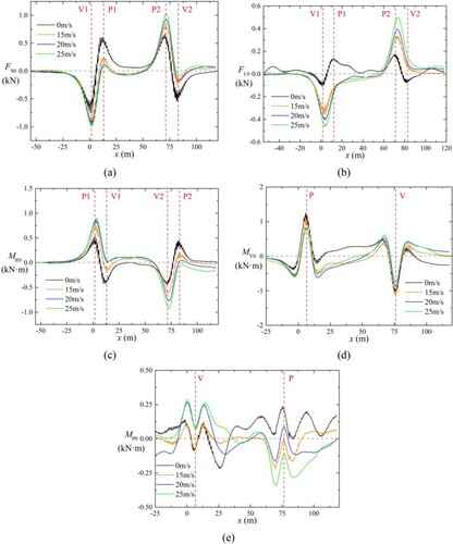
According to Figure 22, it could be seen that for F_S0 and M_R0, the increasing wind speed enhances the first peak/valley value and weakens the second one. Therefore, there is limited influence on the variation amplitude of F_S0 and M_R0. Due to the reduction in the second peak/valley value, the F_S0 and M_R0 when the van traveling around the middle carriage are closer to the ones in the sole-traveling condition. A similar phenomenon could also be seen in M_Y0. For the M_Y0, the first and the third peak/valley value have been increased, and the second peak/valley value has been weakened. The variation amplitude doesn’t vary a lot neither. The variation amplitude of F_L0 varies a lot when wind speed changes. When there is no wind, two peak/valley values could be observed in each major variation, and the variation contains fiercer fluctuation, which shortens the length of the plateau stage. The crosswind has eliminated the second peak/valley value. Instead, it produces a slope between the P1 and P2, and the variation amplitude increases with the wind speed. As for M_P0, it contains a fierce oscillation in the curves, and the variation amplitude seems not to be influenced by the wind speed.

According to Figure 22, it could be seen that the wind speed has a more pronounced influence on F_S0, F_L0 and M_R0. Quantitative analysis is given in Table 11, for F_S0 and M_R0, P1, V1 and their difference value are extracted. For F_L0, V1 is extracted under the crosswind condition, the difference value of V1-P1 is extracted at the wind speed of 0 m/s.

Table 11. Peak/valley values and variation amplitudes at different wind speeds (Unit: kN, kN·m).

No. of Case		1	2	3	4
FS	V1	−0.7598	−0.9665	−0.9471	−0.9969
	P1	0.6070	0.2302	0.1204	0.0946
	P1-V1	1.3668	1.1967	1.0675	1.0914
FL	V1	−0.2013	−0.3583	−0.4038	−0.4638
MR	V1	−0.4246	−0.1539	0.0196	0.0166
	P1	0.5489	0.7646	0.8513	0.8967
	P1-V1	0.9735	0.9185	0.8317	0.8801

As can be seen in Table 11, for F_S0 and M_R0, case 1 gets the largest variation amplitude, and the variation amplitude at different wind speeds is close. For F_S0, the variation amplitude of case 1 is about 1.2 times of case 2 ∼ 4; for M_R0, the variation amplitude of case 1 is about 1.1 times of case 2 ∼ 4. It is noteworthy that the crosswind has increased the proportion of the first peak/valley value. For F_S0, the proportion of the first peak/valley value in the variation amplitude increases from 55% in case 1–91% in case 4. While for M_R0, the aerodynamic variation from the sole-traveling state to P1 gradually becomes the largest variation amplitude. For F_L0, the variation amplitude increases with the wind speed. Compared to case 1, when the wind speed increases by 5 m/s, the variation range increases by about 0.05kN.

Among the aerodynamic forces of road vehicles, F_S determines the sideslip, M_R determines the rollover and M_Y controls the lateral deviation (Dorigatti et al., 2015). In contrast, the influence of F_L and M_P is limited. Through the above analysis, since the variation amplitudes at the wind speed of 0 m/s are about 1.1 ∼ 1.2 times of the ones under the crosswind condition, acquiring the aerodynamic forces by adding the aerodynamic variations at the wind speed of 0 m/s to the sole-traveling state at any wind speeds is conservative. It would produce a quick and comparatively accurate reference to actual engineering.

5. Conclusions

This work has developed a numerical model to identify the aerodynamic loads of road vehicles when traveling on a single-level rail-cum-road bridge under crosswind and train-induced wind. The simulation's accuracy has been validated by the comparison with large-scale wind tunnel tests, moving model tests, and existing relevant wind tunnel tests. The flow features on the vehicle-bridge system, the influence of train-induced wind on different lanes and vehicles, and the superposition effect of crosswind and train-induced wind have been systematically analyzed. The main discoveries are summarized as follows:

1. The superposition of train-induced wind and the crosswind occurs at the windward side of the concrete wall. The superposed area develops along the concrete wall, producing two high-pressure zones and two low-pressure zones near the train nose and train tail that significantly change the aerodynamics of road vehicles.

2. The flow feature near the moving train brings two major aerodynamic variations for the road vehicles near the train nose and train tail. The relatively stable pressure zone around the middle carriage provides a plateau. In each major variation, the train-induced load changes direction two times in F_S and M_R, one time in F_L and three times in M_Y. In contrast, the aerodynamic load of M_P has a constant fluctuation due to the separation flow of the upstream bridge flange and the train-induced wind.

3. For the three windward lanes, the closer it is to the railway, the smaller the static wind load is, while the influence from the train-induced wind is more significant. The variation amplitude of C_S, C_MR and C_MY on lane 1 and lane 2 is about 30% and 40% of that on lane 3. For lane 1 ∼ lane 3, the aerodynamic amplitude of C_S and C_MR induced by the train wind is about 10%, 20% and 50% of the static wind load at the wind speed of 15 m/s, respectively. The variation amplitude of C_MY on lane 3 is about 1.5 times the static wind load.

4. Due to their similar height, the discussed three road vehicles possess similar C_S, C_L and C_MR under the sole-traveling condition, while C_MY varies obviously with the vehicle length. Similar phenomenon exists in the variation amplitude under the train-induced wind. The variation amplitude of C_S and C_L of the three vehicles is about 0.1 and 0.05, and the variation amplitude of C_MR is about 0.05 ∼ 0.1. The longer the vehicle is, the variation amplitude of C_MY and C_MP is larger. The truck trailer gets the largest variation amplitude of C_MY and C_MR of 0.4761 and 0.0871, respectively.

5. The variation trend of C_S, C_L, C_MR and C_MP with the wind yaw angle on the single-level rail-cum-road bridge is similar to the results on the ground and a traditional box girder. Since the highway is further from the windward flange of the bridge, the change in wind yaw angle has little influence on C_MY.

6. The crosswind would decrease the variation amplitude of C_S, C_MR and C_MY by 10% ∼ 20%, while the influence on the variation of C_L and C_MP is limited. Therefore, the aerodynamic forces of the vehicle during meeting the train at different wind speeds can be quickly obtained by superimposing the aerodynamic variation caused by the moving train at the wind speed of 0 m/s and the aerodynamic forces at its sole-traveling state. The results are conservative and can provide a valuable reference for relevant actual engineering.

Since the road vehicles in the present research have a common high-sided feature, other road vehicles with different features are worth discussing. Moreover, exploring the wind-resistant effect of bridge deck system would be helpful for the deck layout of single-level rail-cum-road bridges. In our future work, wind-car-train-bridge coupled system will be developed to discuss the response of the vehicle-bridge system under actual traveling condition.

Disclosure statement

No potential conflict of interest was reported by the author(s).

Additional information

Funding

This work was supported by National Natural Science Foundation of China: [grant numbers 51778544, 51978589, 51908077]; Chinese Universities Scientific Fund: [grant number 2682021CG014].

References

- Alonso-Estébanez, A., Del Coz Díaz, J. J., Álvarez Rabanal, F. P., & Pascual-Muñoz, P. (2017). Numerical simulation of bus aerodynamics on several classes of bridge decks. Engineering Applications of Computational Fluid Mechanics, 11, 435–449. https://doi.org/10.1080/19942060.2016.1201544
- Alonso-Estébanez, A., Juan, J., Dí, C., & Rabanal, FPÁ. (2018). Numerical investigation of truck aerodynamics on several classes of infrastructures. Wind and Structures, 26, 35–43. https://doi.org/10.12989/was.2018.26.1.035
- Baker, C. J. (1988). High sided articulated road vehicles in strong cross winds. Journal of Wind Engineering and Industrial Aerodynamics, 31(1), 67–85. https://doi.org/10.1016/0167-6105(88)90188-2
- Baker, C. J., & Reynolds, S. (1992). Wind-induced accidents of road vehicles. Accident Analysis & Prevention, 24(6), 559–575. https://doi.org/10.1016/0001-4575(92)90009-8
- Broniszewski, J., & Piechna, J. (2019). A fully coupled analysis of unsteady aerodynamics impact on vehicle dynamics during braking. Engineering Applications of Computational Fluid Mechanics, 13, 623–641. https://doi.org/10.1080/19942060.2019.1616326
- Chen, N., Li, Y., Wang, B., Su, Y., & Xiang, H. (2015). Effects of wind barrier on the safety of vehicles driven on bridges. Journal of Wind Engineering and Industrial Aerodynamics, 143, 113–127. https://doi.org/10.1016/j.jweia.2015.04.021
- Chen, Y. G., & Wu, Q. (2018). Study on unsteady aerodynamic characteristics of two trains passing by each other in the open air. Journal of Vibroengineering, 20(2), 1161–1178. https://doi.org/10.21595/jve.2018.18695
- Cheung, M. M. S., & Chan, B. Y. B. (2010). Operational requirements for long-span bridges under strong wind events. Journal of Bridge Engineering, 15(2), 131–143. https://doi.org/10.1061/(ASCE)BE.1943-5592.0000044
- Dorigatti, F., Sterling, M., Baker, C. J., & Quinn, A. D. (2015). Crosswind effects on the stability of a model passenger train—A comparison of static and moving experiments. Journal of Wind Engineering and Industrial Aerodynamics, 138, 36–51. https://doi.org/10.1016/j.jweia.2014.11.009
- Dorigatti, F., Sterling, M., Rocchi, D., Belloli, M., Quinn, A. D., Baker, C. J., & Ozkan, E. (2012). Wind tunnel measurements of crosswind loads on high sided vehicles over long span bridges. Journal of Wind Engineering and Industrial Aerodynamics, 107–108, 214–224. https://doi.org/10.1016/j.jweia.2012.04.017
- Ghalandari, M., Shamshirband, S., Mosavi, A., & Chau, K. W. (2019). Flutter speed estimation using presented differential quadrature method formulation. Engineering Applications of Computational Fluid Mechanics, 13, 804–810. https://doi.org/10.1080/19942060.2019.1627676
- Han, Y., Huang, J., Cai, C. S., Chen, S., & He, X. (2019). Driving safety analysis of various types of vehicles on long-span bridges in crosswinds considering aerodynamic interference. Wind and Structures, 29, 279–297. https://doi.org/10.12989/was.2019.29.4.279
- Han, Y., Li, K., Chen, H., Cai, C. S., & Dong, G. C. (2018). Numerical simulation on aerodynamic characteristics of typical vehicles on bridges and the windshield effects between vehicles. Gongcheng Lixue/Engineering Mech, 35, https://doi.org/10.6052/j.issn.1000-4750.2017.01.0002
- Huang, S., Li, Z., & Yang, M. (2019). Aerodynamics of high-speed maglev trains passing each other in open air. Journal of Wind Engineering and Industrial Aerodynamics, 188, 151–160. https://doi.org/10.1016/j.jweia.2019.02.025
- Jasak, H. (2009). Dynamic Mesh Handling in OpenFOAM. 47th AIAA aerospace sciences meeting including the new horizons forum and aerospace exposition. https://doi.org/10.2514/6.2009-341.
- Kim, S. J., Shim, J. H., & Kim, H. K. (2020). How wind affects vehicles crossing a double-deck suspension bridge. Journal of Wind Engineering and Industrial Aerodynamics, 206, 104329. https://doi.org/10.1016/j.jweia.2020.104329
- Li, W., Liu, T., Chen, Z., Guo, Z., & Huo, X. (2020). Comparative study on the unsteady slipstream induced by a single train and two trains passing each other in a tunnel. Journal of Wind Engineering and Industrial Aerodynamics, 198, 104095. https://doi.org/10.1016/j.jweia.2020.104095
- Liang, X. F., Li, X. B., Chen, G., Sun, B., Wang, Z., Xiong, X. H., Yin, J., Tang, M. Z., Li, X. L., & Krajnović, S. (2020). On the aerodynamic loads when a high speed train passes under an overhead bridge. Journal of Wind Engineering and Industrial Aerodynamics, 202. https://doi.org/10.1016/j.jweia.2020.104208
- Liu, T., Chen, Z., Zhou, X., & Zhang, J. (2018). A CFD analysis of the aerodynamics of a highspeed train passing through a windbreak transition under crosswind. Engineering Applications of Computational Fluid Mechanics, 12, 137–151. https://doi.org/10.1080/19942060.2017.1360211
- Menter, F. R., Kuntz, M., & Langtry, R. (2003). Ten years of industrial experience with the SST turbulence model. Turbulence Heat and Mass Transfer, 4, 625–632. https://cfd.spbstu.ru/agarbaruk/doc/2003_Menter,%20Kuntz,%20Langtry_Ten%20years%20of%20industrial%20experience%20with%20the%20SST%20turbulence%20model.pdf
- Niu, J., Zhou, D., & Liang, X. (2018). Numerical investigation of the aerodynamic characteristics of high-speed trains of different lengths under crosswind with or without windbreaks. Engineering Applications of Computational Fluid Mechanics, 12, 195–215. https://doi.org/10.1080/19942060.2017.1390-786
- Prewitt, N. C., Belk, D. M., & Shyy, W. (2000). Parallel computing of overset grids for aerodynamic problems with moving objects. Progress in Aerospace Sciences, https://doi.org/10.1016/S0376-0421(99)00013-5
- Salati, L., Schito, P., & Cheli, F. (2019). Strategies to reduce the risk of side wind induced accident on heavy truck. Journal of Fluids and Structures, 88, 331–351. https://doi.org/10.1016/j.jfluidstructs.2019.05.004
- Salati, L., Schito, P., Rocchi, D., & Sabbioni, E. (2018). Aerodynamic study on a heavy truck passing by a bridge pylon under crosswinds using CFD. Journal of Bridge Engineering, 23(9), 04018065. https://doi.org/10.1061/(ASCE)BE.1943-5592.0001277
- Salih, S. Q., Aldlemy, M. S., Rasani, M. R., Ariffin, A. K., Ya, T. M. Y. S. T., Al-Ansari, N., Yaseen, Z. M., & Chau, K. W. (2019). Thin and sharp edges bodies-fluid interaction simulation using cut-cell immersed boundary method. Engineering Applications of Computational Fluid Mechanics, 13, 860–877. https://doi.org/10.1080/19942060.2019.1652209
- Schober, M., Weise, M., Orellano, A., Deeg, P., & Wetzel, W. (2010). Wind tunnel investigation of an ICE 3 endcar on three standard ground scenarios. Journal of Wind Engineering and Industrial Aerodynamics, 98(6-7), 345–352. https://doi.org/10.1016/j.jweia.2009.12.004
- Sun, Z., Zhang, Y., Guo, D., Yang, G., & Liu, Y. (2014). Research on running stability of CRH3 high speed trains passing by each other. Engineering Applications of Computational Fluid Mechanics, 8, 140–157. https://doi.org/10.1080/19942060.2014.11015504
- Suzuki, M., Tanemoto, K., & Maeda, T. (2003). Aerodynamic characteristics of train/vehicles under cross winds. Journal of Wind Engineering and Industrial Aerodynamics, 91(1-2), 209–218. https://doi.org/10.1016/S0167-6105(02)00346-X
- Tokunaga, M., Sogabe, M., Santo, T., & Ono, K. (2016). Dynamic response evaluation of tall noise barrier on high speed railway structures. Journal of Sound and Vibration, 366, 293–308. https://doi.org/10.1016/j.jsv.2015.12.015
- Wang, B., Xu, Y., Zhu, L., Cao, S., & Li, Y. (2013). Determination of aerodynamic forces on stationary/moving vehicle-bridge deck system under crosswinds using computational fluid dynamics. Engineering Applications of Computational Fluid Mechanics, 7(3), https://doi.org/10.1080/19942060.2013.11015477
- Wang, Y., & Saul, R. (2020). Wide cable-supported bridges for rail-cum-road traffic. Structural Engineering International, 30, 551–559. https://doi.org/10.1080/10168664.2020.1735-980
- Wang, Y., Zhang, Z., Zhang, Q., Hu, Z., & Su, C. (2021). Dynamic coupling analysis of the aerodynamic performance of a sedan passing by the bridge pylon in a crosswind. Applied Mathematical Modelling, 89, 1279–1293. https://doi.org/10.1016/j.apm.2020.07.003
- Xiang, H., Li, Y., Chen, S., & Li, C. (2017). A wind tunnel test method on aerodynamic characteristics of moving vehicles under crosswinds. Journal of Wind Engineering and Industrial Aerodynamics, 163, 15–23. https://doi.org/10.1016/j.jweia.2017.01.013
- Xiang, H., Li, Y., Wang, B., & Liao, H. (2015). Numerical simulation of the protective effect of railway wind barriers under crosswinds. International Journal of Rail Transportation, 3(3), 151–163. https://doi.org/10.1080/23248378.2015.105-4906
- Xiong, X. H., Li, A. H., Liang, X. F., & Zhang, J. (2018). Field study on high-speed train induced fluctuating pressure on a bridge noise barrier. Journal of Wind Engineering and Industrial Aerodynamics, 177, 157–166. https://doi.org/10.1016/j.jweia.2018.04.017
- Yang, N., Zheng, X. K., Zhang, J., Law, S. S., & Yang, Q. S. (2015). Experimental and numerical studies on aerodynamic loads on an overhead bridge due to passage of high-speed train. Journal of Wind Engineering and Industrial Aerodynamics, 140, 19–33. https://doi.org/10.1016/j.jweia.2015.01.015
- Yang, W., Deng, E., Lei, M., Zhu, Z., & Zhang, P. (2019). Transient aerodynamic performance of high-speed trains when passing through two windproof facilities under crosswinds: A comparative study. Engineering Structures, 188, 729–744. https://doi.org/10.1016/j.engstruct.2019.03.070
- Yao, Z., Zhang, N., Chen, X., Zhang, C., Xia, H., & Li, X. (2020). The effect of moving train on the aerodynamic performances of train-bridge system with a crosswind. Engineering Applications of Computational Fluid Mechanics, 14, 222–235. https://doi.org/10.1080/19942060.2019.1704886
- Zhou, D., Tian, H. Q., Zhang, J., & Yang, M. Z. (2014). Pressure transients induced by a high-speed train passing through a station. Journal of Wind Engineering and Industrial Aerodynamics, 135, 1–9. https://doi.org/10.1016/j.jweia.2014.09.006
- Zhou, Q., & Zhu, L. D. (2020). Numerical and experimental study on wind environment at near tower region of a bridge deck. Heliyon, 6(5), e03902. https://doi.org/10.1016/j.heli-yon.2020.e03902
- Zhu, L. D., Li, L., Xu, Y. L., & Zhu, Q. (2012). Wind tunnel investigations of aerodynamic coefficients of road vehicles on bridge deck. Journal of Fluids and Structures, 30, 35–50. https://doi.org/10.1016/j.jfluidstructs.2011.09.002
- Zou, S., He, X., & Wang, H. (2020). Numerical investigation on the crosswind effects on a train running on a bridge. Engineering Applications of Computational Fluid Mechanics, 14, 1458–1471. https://doi.org/10.1080/19942060.2020.1832920
- Zou, Y., Fu, Z., He, X., Cai, C., Zhou, J., & Zhou, S. (2019). Wind load characteristics of wind barriers induced by high-speed trains based on field measurements. Applied Sciences, 9, https://doi.org/10.3390/app9224865