Research on aerodynamic optimization design method and flow mechanism of a high-subsonic compressor cascade

ABSTRACT

Designing the high-performance, high-subsonic airfoils suitable for different Reynolds number flow is the major challenge for high-altitude long-endurance drones and ultra-high altitude solar aircraft. To overcome the difficulties, this paper proposed a set of aerodynamic optimization design methods that combine the improved category shape function transformation method, parallel computational fluid dynamics, and an improved whale optimization algorithm. This approach achieves high modeling accuracy, computational efficiency, and strong optimization ability. Verification using single-peak, multi-peak, and fixed-dimensional test functions demonstrates that the improved whale optimization algorithm has significantly enhanced optimization capabilities compared with the conventional whale optimization, particle swarm optimization, and gravity search algorithms. Numerical simulations are used to analyze the internal flow mechanisms before and after airfoil optimization under different Reynolds numbers. The results show that, compared with the original airfoil, the optimized airfoil has front loading characteristics that effectively reduce the adverse pressure gradient of the rear part of suction surface, promoting the transition in this region. The reduced adverse pressure gradient also inhibits the development and growth of laminar separation bubbles and slows down the growth of the boundary layer displacement thickness, thereby reducing wake mixing loss and improving the aerodynamic performance.

KEYWORDS:

• Optimization design
• high-subsonic airfoil
• improved whale optimization algorithm
• boundary layer displacement thickness
• Reynolds number

Nomenclature

a	=	Convergence factor
ava	=	Average value
B	=	Bezier spline curve
C	=	Chord length
Cax	=	Axial chord length
Cal	=	Calculation results
CDA	=	Controlled diffusion airfoil
CDM	=	Conjugate direction method
CFD	=	Computational fluid dynamics
Cf	=	Skin friction coefficient
Cp	=	Blade loading coefficient
Dpitch	=	Pitch distance
GA	=	Genetic algorithm
H12	=	Boundary layer shape factor
LE	=	Leading edge
LSB	=	Laminar separation bubble
m	=	Meter
Ma	=	Mach number
N	=	Iteration number
Ori	=	Original cascade
Opt	=	Optimized cascade
PS	=	Pressure surface
$P{s}_{in}$	=	Inlet static pressure
Pt	=	Total pressure
Ptin	=	Inlet total pressure
$P{t}_{out}$	=	Outlet total pressure
RANS	=	Reynolds averaged Navier–Stokes
Re	=	Reynolds number
std	=	Standard deviation
SOP	=	Second order polynomial
SS	=	Suction surface
TE	=	Trailing edge
TKE	=	Turbulent kinetic energy
x	=	Axial length
y	=	Pitch length
$\omega$	=	Total pressure loss coefficient
$\omega (t)$	=	Inertia weight
${\delta }^{\ast }$	=	Boundary layer displacement thickness
$\theta$	=	Boundary layer momentum thickness

1. Introduction

Due to the rapid development of high-altitude long-endurance unmanned aerial vehicles (UAV) and ultra-high altitude solar aircraft, there is an urgent need for high aerodynamic, high-subsonic performance airfoils for low Reynolds number. However, at low Reynolds numbers (Re = 10⁴∼10⁵), the fluid transitions to turbulent flow through laminar separation bubbles (LSBs) in the presence of an adverse pressure gradient, and then separates from blade surface, which significantly deteriorates the aerodynamic performance and stable working range of the airfoil (Lissaman, 1983). Therefore, it is important to consider the design of high-performance airfoils suitable for different Re flows that suppress the influence of Re on the aerodynamic performance. At present, such a design is one of the technical bottlenecks to improving the performance of future airfoils. Thus, the optimization of airfoil designs under different Re conditions has become an important part of the aerodynamic design of airfoils. An optimization method would shorten the design cycle and reduce the cost of the aerodynamic design of airfoils. Such a design method would also effectively reduce the dependence on manual design experience, further improving the aerodynamic design level of airfoils. Research shows that optimization design faces three major problems: the high-dimensionality of the problem, the time-consuming design process, and the black-box nature of the optimization approach (Shan & Wang, 2010). Considerable research has been undertaken to overcome these three problems, with most studies focusing on one of the following three aspects: aerodynamic shape parameterization with high modeling accuracy, fast or accurate numerical methods, and optimization algorithms with strong optimization ability (Dirk et al., 2003).

In terms of aerodynamic shape parameterization, the traditional modeling method involves changing the blade shape of different sections and three-dimensional stacking characteristics along the normal direction of the center of gravity of each section. The shape of the airfoils has had four main stages of development. The first stage was from the 1960s to the 1970s, when countries such as the UK, the USA, and the Soviet Union proposed the C4 airfoil, NACA65 airfoil, and BC6 airfoil, respectively. The common point of these standard airfoils is that the mean camber lines are all parabolic. The second stage was from the 1970s to the 1980s, when the double circular arc profiles and multi-circular arc profiles were developed. The mean camber lines in these cases are composed of two arcs. The third stage saw the introduction of the controlled diffusion airfoil (CDA) and arbitrary polynomial airfoil, which have been widely studied (Shreeve et al., 1991; Song et al., 2008; Steinert et al., 1991). The latest stage of development has seen new aerodynamic shape parameterization methods such as class shape transformation (CST), parametric section (PARSEC), and the free deformation method (FFD) (John et al., 2016; Kulfan & Bussoletti, 2006; Sobieczky, 1999). In 1984, Hobbs and Weingold (1984) found through experimental research: compared with the traditional NACA65 airfoil, the CDA airfoil has a lower flow loss, a higher critical Mach number, and a wider angle of attack range. In 2000, Köller et al. (2000) used a third-order spline function to construct the pressure surface and suction surface, combining a normal distribution random search with the gradient method to optimize the design of several profiles. The results showed that the optimized profile achieved lower flow losses than the original profile, and had an increased working range in which the total pressure loss was low. In 2003, Burguburu and Le Pape (2003) proposed a novel geometric modeling method in which Bezier surfaces were introduced into the field of internal flow to optimize the rotor of the compressor blade. By using the gradient algorithm, the optimized design achieved an increase in efficiency of more than 1% over an unchanged stable working range. In 2019, Adjei et al. (2019) used the B-spline free deformation parameterization method, the Gaussian process response surface method, and a multi-objective genetic algorithm to optimize a high-load compressor stator. After optimization, the blade has a thinner profile in the middle, which eliminates the local separation vortex, redistributes the secondary flow in the span direction, reduces the corner separation near the suction surface of the hub, and reduces the total pressure loss and the outlet pre-swirl angle by 6.05% and 36.87%, respectively. In terms of numerical calculation technology, a variety of techniques have been developed, such as the MIT airfoil analysis and design system XFOIL (Drela, 1989), DLR 3D aerodynamic calculation program TRACE (Becker et al., 2010), NUMECA FINE solver (Wang et al., 2021) and well-known open-source computational fluid dynamics (CFD) program OpenFOAM (Casartelli & Mangani, 2013). Among them, Hager et al. (1993) pointed out that design optimization should be based on accurate flow simulation to achieve the improvement of actual performance. It is recommended to use a 3D aerodynamic calculation program instead of a 2D Euler simulation when time-consuming is acceptable. Wang et al. (2021) combined the FINE solver, artificial neural network, and genetic algorithm to perform multi-condition optimization calculations on the sweep and lean of a compressor. The calculation results show that the isentropic efficiency and stall margin of the compressor are improved after optimization. In terms of optimization, many local and global algorithms have been studied. Local algorithms mainly include gradient algorithms: Newton’s method, the simplex method, sequential quadratic programming, generalized reduced gradient code, and so on (Levin & Wei, 2001). The main disadvantages of these methods are that they are highly sensitive to the noise of the target and the constraint function, the search process can easily become trapped around a local optimum, and the gradient information of the optimization variables needs to be determined during the optimization process. The computational load is proportional to the number of designs, and the calculation cost is high. The global algorithms mainly include bionic algorithms: the genetic algorithm, particle swarm optimization, firefly algorithm, and so on. These algorithms operate a random search method to simulate the evolution of living organisms or the social behavior of populations. They do not depend on gradient information for the solution, and are very robust to the initial solution. With their characteristics of intergenerational inheritance and swarm intelligence, they are suitable for large-scale complex optimization problems and have a wide field of applications. Sanger (1983) introduced the optimized technology into compressor aerodynamic design for the first time, and successfully used a local optimization algorithm to effectively reduce the boundary layer shape factor and flow separation, thereby improving the aerodynamic performance of a compressor airfoil. Subsequently, with the development of CFD techniques, the aerodynamic shape design of compressors has entered the era of three-dimensional numerical optimization. Research by Behlke (1985) showed that the efficiency and stall margin of a multi-stage compressor could be increased by 1.5% and 8%, respectively, by using the second-generation CDA airfoil and considering the end wall loss. Jeong et al. (2005) applied a Kriging-based genetic algorithm to the aerodynamic design of a two-dimensional airfoil. Hergt et al. (2013) applied a multi-objective genetic algorithm to optimize the shape of a highly deflected compressor blade under various conditions. The research results show that, compared with the prototype, the blade loading characteristics of the optimized cascade move forward, and the flow loss is reduced under low Re conditions. Luo et al. (2014) applied the adjoint method to an axial compressor rotor. Baert et al. (2017) proposed an innovative adaptive proxy model for high-dimensional and highly constrained design problems, and applied interpolation/regression and classification fusion to the integrated optimization platform MINAMO. Taking the NASA 37 rotor as an example, optimization of 60 design parameters under 30 constraints led to increases of 3.5% and 2% in the adiabatic efficiency and the stall margin, respectively. Then, Duan et al. (2019) and Cheng et al. (2019) used particle swarm optimization and an improved artificial bee colony algorithm, respectively, to optimize the NASA 37 compressor rotor. Both optimization strategies achieved adiabatic efficiency enhancements of more than 1%.

From the above summary of optimization design methods in the field of airfoils, it can be seen that modern optimization design methods are developing in three directions. The first direction involves improving aerodynamic shape parameterization methods, seeking aerodynamic shape design requirements with high modeling accuracy, effectively reducing the number of optimization variables, and improving the efficiency of optimization design. The second direction focuses on improving the numerical solution tools and using a variety of acceleration techniques to speed up the calculation process. The third direction seeks improved optimization algorithms, enhanced optimization ability and convergence speed, shorter optimization design times, and improved optimization speed.

Although there has been some research on optimization, the optimization of high-subsonic airfoils suitable for a range of Re flows still requires a fast and accurate optimization design method with strong optimization ability. And to date, there has been no unified conclusion about the blade shape design of high-subsonic airfoils suitable for different Re conditions. Therefore, this paper put forwards the improved class shape function transformation method, a CFD-based solution approach, and an improved whale optimization algorithm to design a high-subsonic airfoil suitable for different Re values. We study the internal mechanism between the flow structure of LSBs and flow loss of cascades before and after optimization, and thus identify the complex internal flow mechanisms that occur before and after cascade optimization under different Re conditions.

2. Numerical framework

2.1. Compressor cascade

A high-subsonic V103 compressor airfoil is taken as the research object in the present study (Steinert et al., 1991). Figure 1 shows the sketch map of V103 compressor airfoil. The aerodynamic and geometry parameters are listed in Table 1. The compressor airfoil V103 has a design inlet Mach number of Ma₁= 0.67, inlet flow angle of β₁= 132° (design incidence i = 0°), and installation angle of β_s=  112.5°.

Figure 1. Sketch map of V103 compressor airfoil.

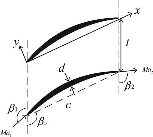
Table 1. Aerodynamic and geometry parameters of compressor airfoil V103.

Design value	Value
Inlet Mach number Ma1	0.67
Chord length c/(m)	0.18
Solidity c/t	1.82
Inlet airflow angle β1/(°)	132
Outlet airflow angle β2/(°)	96
Stagger angle βs/(°)	112.5
Diffusion factor D	0.415
Reynolds number Re	4.5 × 10^5

2.2. Blade profile parameterization method

The original CST method was proposed by Kulfan and Bussoletti (2006). Research shows that the CST method has the advantages of strong robustness, few design parameters, and high modeling accuracy. The CST method uses the product of class functions and shape functions, plus a function that expresses the characteristics of trailing edge to fit blade profile. The details are as follows: (1) $\xi (\mathrm{\Psi })=\text{C}(\mathrm{\Psi })\text{S}(\mathrm{\Psi })+\mathrm{\Psi }\mathrm{\Delta }\zeta$(1) where $\mathrm{\Psi }=x{c}^{-1}$ is the dimensionless abscissa of the blade profile, in which x is the abscissa and c is the chord length; $\zeta =y{c}^{-1}$ is the dimensionless ordinate of blade profile, in which y is the ordinate; and $\mathrm{\Delta }\zeta =\mathrm{\Delta }{y}_{TE}{c}^{-1}$ is the dimensionless trailing edge thickness of the blade profile, in which $\mathrm{\Delta }{y}_{TE}$ is the thickness.

$C(\mathrm{\Psi })$ is a class function describing the blade geometry, the details are as follows: (2) $C(\mathrm{\Psi })={\mathrm{\Psi }}^{N_1}(1-\mathrm{\Psi }{)}^{N_2}$(2) where $N_1$, $N_2$ are control coefficients, usually 0.5, 0.75, or 1, different values of which correspond to different basic shapes.

$S(\mathrm{\Psi })$ is a shape function of the blade geometry correction. In this paper, the weighted sum of Bernstein polynomials of order n is adopted. This has the following form: (3) $S(\mathrm{\Psi })=\sum _{r=0}^n{A}_r\frac{n!}{r!(n-r)!}{\mathrm{\Psi }}^r(1-\mathrm{\Psi }{)}^{n-r}$(3) where r is the exponent of Bernstein polynomial; n is the order of Bernstein polynomial; Ar is the corresponding weight factor.

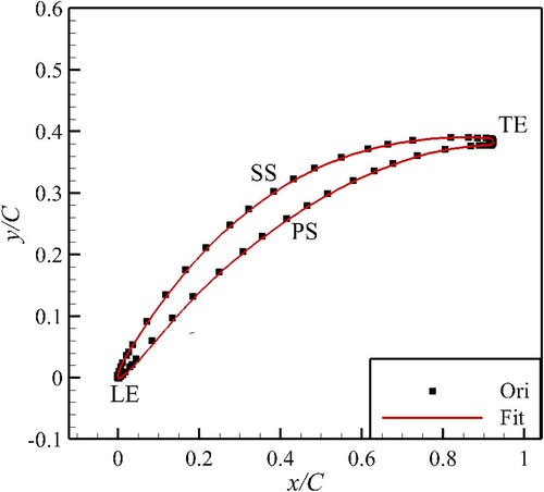
However, if the CST method is used, the control coefficients $N_1$ and $N_2$ are both 0.5, and the max fitting error is 1.3 × 10⁻² m, which does not meet the error requirements for wind tunnel models. In this paper, we propose an improved class shape transformation (ICST) approach. In the ICST method, the control coefficients $N_1$ and $N_2$ are taken as unknowns, and the least-squares method is used to overcome the low fitting accuracy of the CST method at the leading edge and trailing edge. The improvement of the flexible control coefficients in ICST method is one of the innovations of airfoil design in this paper, which can greatly improve the accuracy of airfoil fitting and has wide applicability to different airfoils. Considering the fitting accuracy and the optimization time-consuming, the ICST parameterization method with n = 7 is used to fit the compressor cascade geometry. The max fitting error is 5.09 × 10⁻⁴ m, which satisfies the error requirements for wind tunnel models. The fitting results are shown in Figure 2. The pressure surface and suction surface of the blade profile are expressed by different functions $\xi (\mathrm{\Psi })$. After the coordinates of discrete points along the blade profile are known, the weight factors Ar is solved by the least-squares method, and the parametric design process of the blade profile is complete. In the process of numerical optimization, Ar is used as optimization variables to control the shape of the suction surface and pressure surface of the airfoil, as well as the changes in the shape of the leading edge and trailing edge.

Figure 2. Fitting results of V103 compressor airfoil.

2.3. Solution method

In this study, the commercial CFX code is used as the flow solver. This code is based on the finite volume method and a second-order resolution scheme to solve the three-dimensional, steady, and Reynolds averaged Navier–Stokes (RANS) equations. The differential conservation form of the RANS equation in the Cartesian coordinate system is as follows (Abadi et al., 2020; Chen et al., 2019; Ghalandari et al., 2019): (4) $\begin{array}{rl}& \frac{\mathrm{\partial }\rho }{\mathrm{\partial }t}+\frac{\mathrm{\partial }(\rho U_j)}{\mathrm{\partial }{x}_j}=0\end{array}$(4) (5) $\begin{array}{rl}& \frac{\mathrm{\partial }(\rho U_i)}{\mathrm{\partial }t}+\frac{\mathrm{\partial }(\rho U_i{U}_j)}{\mathrm{\partial }{x}_j}\\ & =-\frac{\mathrm{\partial }p}{\mathrm{\partial }{x}_j}+\frac{\mathrm{\partial }}{\mathrm{\partial }{x}_j}\left[\mu \left(\frac{\mathrm{\partial }{U}_i}{\mathrm{\partial }{x}_j}\text{ + }\frac{\mathrm{\partial }{U}_j}{\mathrm{\partial }{x}_i}\right)\right]\end{array}$(5) (6) $\begin{array}{rl}& \frac{\mathrm{\partial }(\rho h_t)}{\mathrm{\partial }t}-\frac{\mathrm{\partial }p}{\mathrm{\partial }t}+\mathrm{\nabla }(\rho U{h}_t)=\mathrm{\nabla }(\lambda \mathrm{\nabla }T)+\mathrm{\nabla }(U\cdot \tau )\end{array}$(6) where $\rho$, $U$, $p$, $T$ denote density, velocity, pressure, and temperature. h_t is the total enthalpy, and $\mathrm{\nabla }(U\cdot \tau )$ represents the work due to viscous stresses. 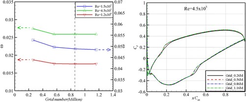To close the control equations, we use the ideal gas state equation: (7) $p=\rho RT$(7) To obtain detailed flow field information and analyze the internal flow loss mechanism of the compressor blade profile under different Re conditions, the shear-stress transport (SST) k-ω model is selected as the turbulence model, and the γ-Re_θ transition model is used to capture the transition phenomenon at different Reynolds numbers. In the numerical calculation, the total pressure, total temperature, and flow direction are applied to inlet boundary, the average static pressure is set at outlet. To study the influence of different Re, the inlet total temperature is kept constant in the numerical calculation, and inlet Re and inlet Ma are changed by adjusting the inlet total pressure and average outlet static pressure to guarantee that both inlet Ma and inlet Re meet the conditions. Figure 3 shows the computational mesh for the V103 compressor cascade. In order to improve the orthogonality of mesh, the O-grids are generated around the blade, and the H-grids are used at the inlet, airfoil passage, and exit. To capture the viscous flow in the boundary layer more accurately, the cell width is set to 1.5 × 10⁻⁶ m so that y⁺ < 1 at the first node away from the solid wall. Periodic conditions are imposed on the circumferential boundary. The solid wall is assigned an adiabatic non-slip boundary condition. To satisfy the grid-independence requirement (Eivaz et al., 2018), the influence of four groups of different grid node numbers (0.26, 0.56, 0.86, 1.16 million) on aerodynamic performance was studied. It can be concluded from Figure 4 that when the number of grid nodes exceeds 0.86 million, the total pressure loss characteristics and blade loading coefficient distribution hardly change. Considering the calculation time and grid-independence requirement, the grid of 0.86 million nodes is finally selected.

Figure 3. Computational mesh for V103 compressor cascade.

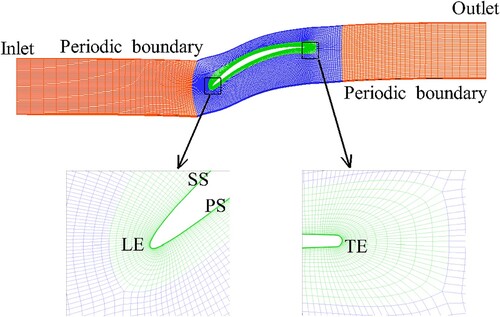
Figure 4. Grid independence for V103 compressor cascade.

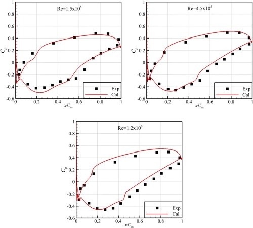
To validate the credibility of the numerical calculations, Figure 5 compares the blade loading coefficient distribution of the V103 compressor cascade under different Re values of the real 2D blade profile. It can be seen that the numerical calculation values are basically consistent with the experimentally measured values (Boese & Fottner, 2002). And the SST k-ω turbulence model coupled with the γ-Reθ transition model accurately captures the ‘platform’ loading distribution characteristics that represent the existence of a separation bubble. The experiment and numerical comparison of (Counsil & Boulama, 2011; Delafin et al., 2014; Seyfert & Krumbein, 2012) also show that the solution model of the CFX can successfully capture details such as LSBs. Therefore, the solution method used to analyze the internal flow mechanism of the compressor blade profile is sufficiently accurate and reliable for this study.

Figure 5. Blade loading coefficient distribution of V103 compressor cascade under different Reynolds numbers.

3. Optimization framework

3.1. Optimization algorithm

Whale optimization is a heuristic algorithm that simulates the predation behavior of whale groups (Mirjalili & Lewis, 2016). The whale optimization algorithm (WOA) has a simple principle, is easy to implement, and has few parameters. The basic principle of WOA is briefly described below. Humpback whales usually prey on fish and shrimp in the ocean by the bubble-net predation method. First, the whales search for quarry at random, and find better quarry by keeping a suitable distance from other whales. Then, the whales identify the location of their quarry, dive to a position about 15 m below the target fish, and move closer to the quarry. Finally, the whales surround their quarry in a spiral, spit out bubbles of different sizes, shrink the radius of the spiral, and force the quarry toward the center of the net. The humpback whales open their mouths upward in an almost upright posture and swallow the quarry in the bubble net. In Addition, it is used by many researchers in different optimization fields. Gharehchopogh and Gholizadeh (2019) systematically summarized the applications of WOA in engineering, classification, image processing, task scheduling, robot path, etc.

To further improve the global optimization ability of the WOA, the initialization strategy, convergence mode, and inertial factor of the WOA are respectively improved to form a novel improved WOA (IWOA) algorithm, which is a further innovative application of the optimization algorithm. The IWOA can greatly improve the optimization ability to search for the optimal value. The innovation of the IWOA in this paper is not only limited to the first application to the turbomachinery optimization problem but also the IWOA algorithm is suitable for various CFD optimization problems. The specific improvements are as follows.

The initial population of WOA is randomly generated in the search space, and the quality of the initialized population has a great influence on the efficiency of the optimization algorithm. A uniformly distributed population is beneficial to expanding the search range, thus improving the convergence speed and accuracy of algorithm. To enhance the individual diversity of population and avoid falling into a local optimum, and considering that chaotic operators are random and regular and not all states can be traversed repeatedly in a certain range, cubic mapping chaotic operators are used to initialize the IWOA population. The cubic mapping chaotic operator is given by the following formula (Gui, 2016): (8) $x_{i+1}=4{x_i}^3-3x_i|x_i|<1\mathrm{\&}{x}_i\ne 0,i=1,2,3\dots$(8) The initialized whale population consists of p n-dimensional whales. The process of initializing the whale population with this cubic mapping is divided into three steps: (1) randomly generate an n-dimensional vector with upper and lower limits of 1 and −1 as the first individual, (2) each dimension of the first individual is iterated to obtain the remaining p-1 individuals according to the above formula 8 and (3) assign the variable values generated by the cubic mappings to a single whale: (9) $X_i=X_{l\text{i}}+(X_{ui}-X_{li})\cdot \frac{x_i\text{ + }1}{2}$(9) where $X_{u\text{i}}$, $X_{l\text{i}}$ are the upper and lower limits of each dimension of each individual, and $X_i$ is the mapped whale individual.

Another important parameter controlling the local search performance and global search performance of WOA is $\overrightarrow{A}$. When $\overrightarrow{A}\ge 1$, the current individual randomly selects other individuals as reference individuals and seeks the optimal solution in the direction of these reference individuals. When $\overrightarrow{A}<1$, the algorithm selects the best whale as the reference whale and seeks the optimal solution in the direction of the reference whale. In this case, the algorithm is no longer conducting a global search, and may become trapped around a locally optimal solution. 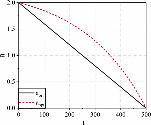$\overrightarrow{A}$ is controlled by a parameter a that decreases linearly in the basic WOA. However, this linear convergence factor is often not conducive to accelerating the algorithm’s optimization process. Therefore, the convergence factor in IWOA is given by: (10) $\text{a}=2-2\left[\left(e^{\frac{2t}{T_{max}}}-1\right)\cdot \frac{1}{e^2-1}\right]$(10) Figure 6 shows the convergence factors before and after this improvement. The improved convergence factor a achieves nonlinear speed attenuation as the number of iterations increases. In the initial stages, the convergence factor decays slowly, which ensures the global search is effective, and then later in the iteration process, the convergence factor decays faster, which improves the speed and efficiency of the local search process. By improving the convergence factor, the optimization capability of the algorithm during the global search is guaranteed to some degree, and optimization efficiency of the algorithm is also accelerated.

Figure 6. Convergence factors before and after improvement.

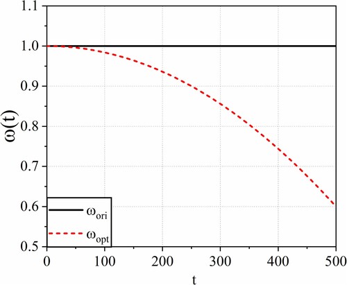
The concept of inertial weight was first applied in particle swarm optimization (PSO) (Li et al., 2012; Lalwani et al., 2013). When the inertial weight is large, the inherited component of the current speed is small, and the particle speed and search range have large ranges. This improves the global search capability of the algorithm, but reduces the local search capability and may prevent the optimal solution from being found. When the inertial weight is small, the inherited component of the current speed is large, and the range over which the particle speed changes is small. In this case, the algorithm searches a certain area finely, but may easily become trapped around a local optimum. Therefore, this paper introduces an inertial weight into IWOA to improve the whale predation behavior. The inertial weight is a decreasing quadratic function of the number of iterations. Figure 7 shows that the rate of change is initially relatively slow, which is conducive to finding the local optimal value that satisfies the conditions in the initial iterations. When approaching the maximum number of iterations, $\omega$ changes rapidly, and quickly converges to the global optimal value after finding the local optimal value, thereby improving operation efficiency. The inertial weight function applied in IWOA is as follows: (11) $\omega (t)=1-\frac{0.4}{{T_{max}}^2}{t}^2$(11) The search process of IWOA can be written as: (12) $\begin{array}{rl}\overrightarrow{X^{\mathrm{\prime }}}(t+1)& =w(t)\cdot \overrightarrow{X^{\ast }}(t)-\overrightarrow{A}\bullet \overrightarrow{D}p<0.\text{5}\end{array}$(12) (13) $\begin{array}{rl}\overrightarrow{X^{\mathrm{\prime }}}(t+1)& =\overrightarrow{D^{\mathrm{\prime }}}{e}^{\text{bl}}\cdot \cos (2\pi l)+w(t)\cdot \overrightarrow{X^{\ast }}(t)p\ge 0.5\end{array}$(13) (14) $\begin{array}{rl}\overrightarrow{X}(t+1)& =\omega (t)\overrightarrow{X_{\text{rand}}}-\overrightarrow{A}\bullet \overrightarrow{D}\end{array}$(14)

Figure 7. Inertia weight before and after improvement.

A flowchart of IWOA is shown in Figure 8. To verify the effectiveness and superiority of IWOA, three benchmark test functions are used to compare the optimization results given by PSO, the gravity search algorithm (GSA), WOA, and IWOA. The three representative test functions selected for this evaluation are a unimodal test function $F_1(x)$, a multimodal test function $F_2(x)$, and a fixed-dimension function $F_3(x)$. Table 2 presents the definitions of these three test functions. For all the test functions, the population size and the maximum number of iterations N_max are uniformly set to 30 and 500, respectively, and each function is tested 30 times. If the average value obtained by the algorithm is close to the theoretical minimum value, then the algorithm has good optimization ability. A smaller standard deviation over the 30 tests indicates better stability and robustness. Table 3 presents the results of optimizing these benchmark test functions. It can be seen that, compared with PSO, GSA, and WOA, the proposed IWOA achieves a smaller average value and standard deviation, that is, IWOA offers better optimization ability and stability.

3.2. Optimization process

The compressor airfoil optimization process combines Latin hypercube sampling (LHS), the response surface proxy model (RSM), and IWOA, as shown in Figure 9. Set the optimization variables A_r, the LHS number N_L, and the N_max to 10, 200, and 500 under multi-condition optimization, respectively. Considering the strength of the blade, the variation range of the thickness of the blade profile should not be too large. Thus, the variation range of the optimization variable A_r is set to 20%. In the optimization process, the weighted sum of the total pressure loss ω under Reynolds numbers of 1.5 × 10⁵, 4.5 × 10⁵, and 1.2 × 10⁶ constitutes the optimization objective function. It means that each iteration of the optimization objective function needs to carry out the numerical simulation of three conditions. By constraining the pressure ratio and mass rate change within 1%, the total pressure loss of airfoil at different Re conditions is reduced to improve the aerodynamic performance. The expression of the optimization objective function F is as follows: (15) $\begin{array}{rl}\text{F}& =\sum c_{Re}(e^{\omega -{\omega }_{ori}})\\ \text{Re}& =1.5\times {10}^5,4.5\times {10}^5,1.2\times {10}^6\end{array}$(15) where $\omega$, $\pi$, and the subscript ori represent the total pressure loss, static pressure ratio, and original blade profile, respectively. $c_{Re}$ represents the weight coefficient. Judging the importance of the objective function based on engineering experience, the coefficients under low Re = 1.5 × 10⁵, design Re = 4.5 × 10⁵, and high Re = 1.2 × 10⁶ are 0.3, 0.4, and 0.3 respectively. Then use RSM to obtain the functional relationship between independent variables that is the optimization variables and dependent variables that is the objective functions. After calculation, the criterion value of RSM is 97.5%. Finally, the IWOA is used to obtain the optimal objective function and the corresponding optimization variable. Using these optimized variable values and the ICST parameterization method, the optimal blade geometry is obtained. Table 4 compares the calculation costs of different optimization examples. It can be seen that the calculation cost of this paper is low enough to be acceptable for engineering calculations.

Figure 8. Flowchart of IWOA.

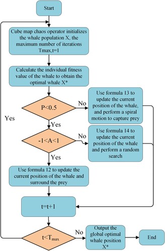
Figure 9. Optimization process for compressor blade profile.

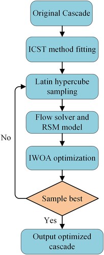
Table 2. Benchmark functions.

Benchmark test function	Dimensions	Domain of definition	Minimum value
Sphere function $F_1(x)=\sum _{i=1}^n{x_i}^2$	30	−100$\sim$100	0
Schwefei function $F_2(x)=\sum _{i=1}^n\left(x_i\sin \left(\sqrt{|x_i|}\right)\right)$	30	−500$\sim$500	−12569.487
Kowalik function $F_3(x)=\sum _{i=1}^{11}{\left[a_i-\frac{x_1({b_i}^2+b_i{x}_2)}{{b_i}^2+b_i{x}_3+x_4}\right]}^2$	4	−5$\sim$5	−1.0316

Table 3. Test results on different benchmark functions.

	PSO		GSA		WOA		IWOA
Function	ave	std	ave	std	ave	std	ave	std
F1	1.0765e-07	3.7783e-07	2.4934e-16	1.1062e-16	7.4022e-76	1.7281e-75	3.2555e-119	1.4774e-118
F2	−8391.1794	0	−2591.2965	514.4203	−10085.6164	1564.6977	−11735.9788	1410.4287
F3	0.020363	0	0.0040831	0.0025884	0.00075732	0.00041599	0.00059053	0.00038309

Table 4. Comparison of the calculation costs of different optimization examples.

Example	Optimization framework	Time
3D stacking optimization (Lee & Kim, 2000)	SOP + CFD + CDM	362h
2D airfoils (Peigin & Epstein, 2004)	BSC + CFD + GA	∼hundred h
3D local optimization (Xiang & Chen, 2021)	DFFD + CFD + MIGA	49 h
3D cascade optimization(this paper)	ICST + CFD + IWOA	24 h

4. Results and discussion

4.1. Comparison of geometry and aerodynamic performance before and after blade profile optimization

Figure 10 compares the geometric characteristics of the V103 blade profile before and after optimization. It can be seen that, compared with the prototype, the maximum thickness of the optimized profile has decreased from 5.5% of chord length to 3.1% of chord length, which is still within the thickness range of the conventional compressor stator blade design. The point of maximum thickness has moved from 43.5% of the chord length to 37.5% of the chord length. There is a similar ‘sharp’ leading edge near leading edge of the optimized airfoil. To analyze more comprehensively and accurately, Table 5 lists several basic aerodynamic performance parameters before and after blade profile optimization, such as inlet flow angle, outlet flow angle, incidence angle, lag angle, diffuser factor, etc. It can be seen that curvature of leading edge and trailing edge have changed in the optimization process, which have a role in changing the inlet metal angle and outlet metal angle. After optimization, the incidence angle is increased by 1.5 degrees, and the lag angle is increased by about 1 degree. Therefore, the diffusion factor slightly increases. In short, the optimization design affects the aerodynamic performance by changing the cascade geometry information. If it is further used to design a multi-stage compressor, it is necessary to change the corresponding angle of the downstream components according to the matching relationship under the premise of the same inflow condition to achieve the best aerodynamic performance. For more information about the process of a multi-stage compressor design, please refer to (Huang et al., 2020).

Figure 10. Comparison of geometric characteristics before and after blade profile optimization.

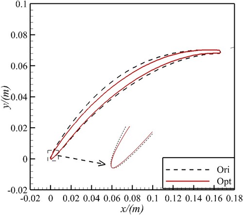
Table 5. Aerodynamic performance parameters before and after blade profile optimization.

Re	Case	β1/(°)	$i$/(°)	β2/(°)	$\delta$/(°)	D
1.5 × 10^5	Ori	132°	0°	99.3°	15.3°	0.397
	Opt	132°	1.5°	98.2°	16.2°	0.404
4.5 × 10^5	Ori	132°	0°	98.3°	14.3°	0.403
	Opt	132°	1.5°	97.5°	15.5°	0.407
1.2 × 10^6	Ori	132°	0°	97.5°	13.5°	0.407
	Opt	132°	1.5°	96.9°	14.9°	0.411

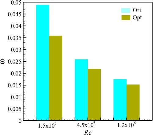
Figure 11 quantifies the total pressure loss characteristics before and after blade profile optimization at different values of Re. The expression of the total pressure loss ω is as follows: (16) $\omega =\frac{P{t}_{in}-P{t}_{out}}{P{t}_{in}-P{s}_{in}}$(16) where $P{t}_{in}$, $P{t}_{out}$, $P{s}_{in}$ denote the inlet total pressure, outlet total pressure, and inlet static pressure, respectively. Compared with the prototype, the ω of the optimized profile has decreased by 26.6%, 15.4%, and 13.1% at Re = 1.5 × 10⁵, 4.5 × 10⁵, and 1.2 × 10⁶, respectively.

Figure 11. Characteristics of total pressure loss before and after blade profile optimization.

4.2. Flow mechanism before and after blade profile optimization

To reveal the mechanism whereby the aerodynamic performance is improved by optimizing the blade profile, the Mach number contours and blade loading distribution before and after blade profile optimization are shown in Figures 12 and 13 for Re = 1.5 × 10⁵, 4.5 × 10⁵, and 1.2 × 10⁶. The expression of the blade loading coefficient C_p is as follows: (17) $C_p=\frac{Ps-P{s}_{in}}{P{t}_{in}-P{s}_{in}}$(17) where $P{t}_{in}$, $P{s}_{in}$, and $Ps$ denote the inlet total pressure, inlet static pressure, and local static pressure of the blade, respectively. Figure 12 indicates that under the same inlet Ma and different Re conditions, the area of high Mach number near the suction surface of the optimized blade profile is smaller than with the original blade profile, and the blade loading moves forward. With Re = 4.5 × 10⁵, the fluid near leading edge of suction side of the original airfoil accelerates, and the velocity peak appears at about 25% of the chord length. A ‘platform’ loading distribution feature then appears from 40∼50% of the chord length, which means separation bubbles occur. According to the Horton separation bubble model (Horton, 1967), the location of the laminar separation point corresponds to the starting point of the ‘platform’ loading. At this time, the boundary layer fluid is very sensitive to disturbance. Then under the disturbances of mainstream, it eventually becomes turbulence. The turbulent boundary layer fluid may reattach to the surface to form turbulent reattachment points. The area surrounded by the laminar separation point and the turbulent reattachment point is called LSB. Figure 13 shows that there are separation bubbles of a certain length on both suction surface and pressure surface of the original compressor cascade. However, due to the sharp leading edge of the optimized blade profile, the airflow reaches its peak velocity near the leading edge of the suction surface and then continues to decelerate to the trailing edge. The loading distribution moves forward, which reduces the streamwise adverse pressure gradient, so that the ‘platform’ loading feature on suction surface and pressure surface does not occur. The reason for this is analyzed in detail below.

Figure 12. Comparison of Mach number before and after blade profile optimization.

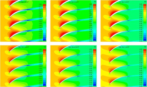
Figure 13. Comparison of blade loading coefficient distribution before and after blade profile optimization.

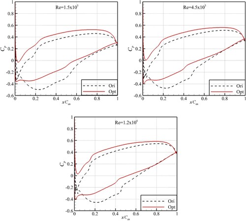
Figure 14 shows the skin friction coefficient C_f on suction surface before and after blade profile optimization. It can be seen that, under different Re values, the optimized profile inhibits the development and growth of LSBs of suction surface compared with the prototype. After optimization, the LSBs of pressure surface are also slightly reduced. Due to space reasons, the analysis will not be repeated here. Table 6 presents the LSB characteristics of suction surface before and after blade profile optimization at Re = 1.5 × 10⁵, 4.5 × 10⁵, and 1.2 × 10⁶. According to Table 6, when Re = 4.5 × 10⁵, laminar separation occurs at 40% of the chord length, turbulent reattachment occurs at 49.2% of the chord length; thus, the LSB length accounts for about 9.2% of the chord length. There is no laminar flow separation on the optimized airfoil, and the LSB disappears. Thus, there is no ‘platform’ loading feature, and the fluid flows well along the whole airfoil passage.

Figure 14. Comparison of skin friction coefficient before and after blade profile optimization.

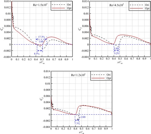
Table 6. LSB characteristics of suction surface before and after blade profile optimization.

Re	Case	LSB Occur (x/Cax)	LSB Reattachment (x/Cax)	Length of LSB (LLSB/Cax)
1.5 × 105	Ori	40.7%	58.0%	17.3%
	Opt	42.8%	51.3%	8.5%
4.5 × 105	Ori	40.0%	49.2%	9.2%
	Opt	/	/	/
1.2 × 106	Ori	38.6%	46.3%	7.7%
	Opt	/	/	/

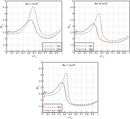
Figure 15 shows the boundary layer shape factor H₁₂ on suction side before and after blade profile optimization. The H₁₂ represents the velocity shape of the boundary layer, which reflects the occurrence of flow separation and flow transition of the boundary layer. The H₁₂ is defined as follows: (18) $H_{12}=\frac{{\delta }^{\ast }}{\theta }$(18) where ${\delta }^{\ast }$ and $\theta$ represent the boundary layer displacement thickness and boundary layer momentum thickness, respectively. Thwaites (1949) and Walker (1975) stated that when H₁₂ exceeds the critical value of 3.7, flow separation occurs on airfoil surface. And the higher the peak value of H₁₂, the more severe the separation of the local flow. As can be seen from Figure 15, the critical H₁₂ corresponding to flow separation, according to the numerical calculations, is basically consistent with the above separation criterion. Compared with the original profile, the peak value of H₁₂ for the optimized profile is much smaller than the critical value, effectively avoiding flow separation.

Figure 15. Comparison of boundary layer shape factors before and after blade profile optimization.

As the loss suffered by the blade suction surface is much greater than that of the pressure surface, Figure 16 shows the distributions of the near-wall velocity field and boundary layer displacement thickness ${\delta }^{\ast }$ over the suction surface before and after blade profile optimization. From Figure 16, we find that the trend in the thickness distribution of LSB is similar to that of ${\delta }^{\ast }$. At the position of maximum LSB thickness, ${\delta }^{\ast }$ has a local extreme value. As Re decreases, the LSB thickness increases, and the ‘displacement’ effect leads to an increase in the turbulent viscous dissipation downstream of the LSB, as well as further thickening of boundary layer and an increasing accumulation of low-energy fluid at the trailing edge. Figure 17 compares the $\theta$ of the suction surface before and after blade profile optimization. After optimization, $\theta$ at trailing edge is significantly lower than in the prototype, and the flow performance of the trailing edge has improved, thereby effectively reducing the flow loss. Figure 18 shows the total pressure ratio at 20% of the chord length downstream of the trailing edge at different Re conditions before and after blade profile optimization. It can be seen that as Re decreases, the wake depth increases. Compared with the prototype profile, the wake depth of the optimized blade profile has decreased at all Re values. To analyze the width and depth of the wake before and after blade shape optimization in a quantitative manner, Table 7 lists the wake depth $\mathrm{\Delta }PR$ and wake width $\mathrm{\Delta }VP$ before and after optimization. $\mathrm{\Delta }PR$ is defined as follows: (19) $\mathrm{\Delta }PR={\left(\frac{P{t}_{out}}{P{t}_{in}}\right)}_{max}-{\left(\frac{P{t}_{out}}{P{t}_{in}}\right)}_{min}$(19) The wake width is given by the width at half of the depth. Table 7 indicates that $\mathrm{\Delta }PR$ in the optimized cascade has been reduced by 2.0%, 0.7%, and 0.6% at Re = 1.5 × 10⁵, 4.5 × 10⁵, and 1.2 × 10⁶, respectively, compared with the original blade profile. $\mathrm{\Delta }VP$ has been reduced by 2.2%, 0.9%, and 0.6%, respectively. This suggests that, as Re decreases, the amplitude of the decrease in $\mathrm{\Delta }PR$ and $\mathrm{\Delta }VP$ after optimization increases. As a result, the extent of the reduction in wake mixing loss also increases. In summary, the increases in the wake mixing loss resulting from displacement effect of LSB is one of the main factors leading to the deterioration of compressor blade profile performance under low-Re conditions. From the velocity field distribution, it can be seen that there is an obvious ‘wedge-shaped’ LSB on suction side of the original profile, but this LSB is suppressed and the growth rate of ${\delta }^{\ast }$ reduces after blade profile optimization. Additionally, both the accumulation of low-energy fluid at the trailing edge and wake mixing loss are reduced, and the aerodynamic performance of airfoil is significantly improved.

Figure 16. Comparison of near-wall velocity field and boundary layer displacement thickness before and after blade profile optimization.

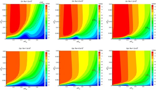
Figure 17. Comparison of boundary layer momentum thickness before and after blade profile optimization.

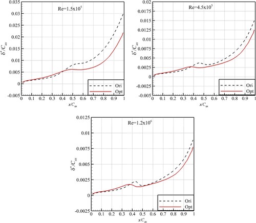
Figure 18. Comparison of total pressure ratio at 20% chord length downstream of trailing edge before and after blade profile optimization.

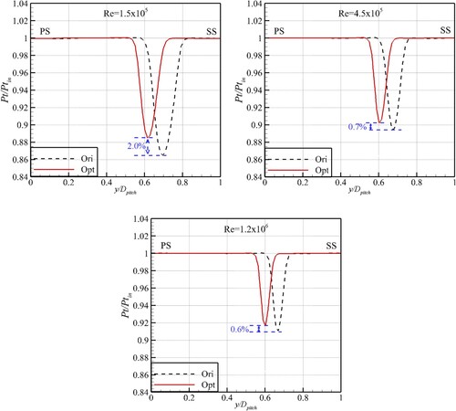
Table 7. Comparison of wake depth and wake width before and after blade profile optimization.

Re	Case	Wake Depth $\mathrm{\Delta }PR$	Wake Width $\mathrm{\Delta }VP$
1.5 × 10^5	Ori	13.5%	11.4%
	Opt	11.5%	9.2%
4.5 × 10^5	Ori	10.5%	7.4%
	Opt	9.8%	6.5%
1.2 × 10^6	Ori	8.9%	5.7%
	Opt	8.3%	5.1%

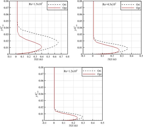
Figure 19 shows the turbulent kinetic energy at 80% of the axial chord length before and after optimization. As Re decreases, the turbulent kinetic energy downstream of the LSB increases rapidly. This main reason is that the LSB becomes thicker and the transition process causes an increase in the degree of mixing between the near-wall fluid and the mainstream downstream of LSB. which in turn leads to a sharp increase in the generation rate of turbulent pulsation. The increased viscous dissipation of the strong turbulence causes the boundary layer to thicken significantly, causing the aerodynamic performance of the compressor cascade to deteriorate.

Figure 19. Comparison of turbulent kinetic energy at 80% axial chord length before and after blade profile optimization.

5. Conclusions

Taking the V103 compressor cascade as the prototype, this paper proposes a set of novel aerodynamic optimization methods to design airfoils suitable for different Re flows, and explores the internal mechanism between the flow structure of LSBs and the flow loss in detail. The main conclusions are as follows: First, a set of optimization design methods that combine the ICST method, parallel CFD, and IWOA proposed in this paper has the advantages of high modeling accuracy, computational efficiency, and strong optimization ability. Verification using single-peak, multi-peak, and fixed-dimensional test functions demonstrated that the optimization ability of IWOA is better than that of WOA, PSO, and GSA. Second, compared with the original cascade, the optimized cascade has a smaller maximum thickness, the position of the maximum thickness has moved forward, and there is a sharp leading edge. The total pressure loss ω of the optimized cascade is 26.6%, 15.4%, and 13.1% lower than that of the original cascade at Re = 1.5 × 10⁵, 4.5 × 10⁵, and 1.2 × 10⁶, respectively. The LSB increases in size as Re decreases. The displacement effect leads to an increase in the turbulent viscous dissipation downstream of the LSB and further thickening of the boundary layer, thus increasing wake mixing loss. This is one of the main factors leading to the deterioration of compressor blade profile performance under low-Re conditions. Third, compared with the prototype, the optimized airfoil has forward loading characteristics under all Re conditions examined in this study. By adjusting the degree of airflow diffusion on suction side, the adverse pressure gradient at the rear part of suction side is effectively reduced. This promotes the transition to occur earlier, inhibits the development and growth of LSBs, and slows the growth of the boundary layer displacement thickness near the trailing edge, which in turn reduces the wake mixing loss and improves aerodynamic performance. Finally, the robustness of the above optimization methods in this study for different turbomachinery cascades and wings needs further study. Future research should focus on the calculation and verification of the above conclusions on various turbomachinery cascades and wings, as well as the continuous improvement of optimization methods, such as the development of advanced aerodynamic shape parameterization composed of combined basis functions and Pareto optimal multi-objective optimization algorithms.

Disclosure statement

No potential conflict of interest was reported by the author(s).

Additional information

Funding

The authors wish to acknowledge the financial support of the National Natural Science Foundation of China [grant number 52106065], and the National Science and Technology Major Projects of China [grant number 2017-II-0010-0024 and 2019-II-0004-0024] for this work.

References

- Abadi, A. M. E., Sadi, M., Farzaneh-Gord, M., Ahmadi, M. H., Kumar, R., & Chau, K. W. (2020). A numerical and experimental study on the energy efficiency of a regenerative heat and mass exchanger utilizing the counter-flow maisotsenko cycle. Engineering Applications of Computational Fluid Mechanics, 14(1), 1–12. https://doi.org/10.1080/19942060.2019.1617193
- Adjei, R. A., Wang, W., & Liu, Y. (2019). Aerodynamic design optimization of an axial flow compressor stator using parameterized free-form deformation. Journal of Engineering for Gas Turbines and Power, 141(10), 1–17. https://doi.org/10.1115/1.4044692
- Baert, L., Beaucaire, P., Leborgne, M., Sainvitu, C., & Lepot, I. (2017). Tackling highly constrained design problems: Efficient optimisation of a highly loaded transonic compressor. ASME Turbo Expo 2017, Charlotte, North Carolina, USA, June 26–30.
- Becker, K., Heitkamp, K., & Kügeler, E. (2010). Recent progress in a hybrid-grid CFD solver for turbomachinery flows. V European Conference on Computational Fluid.
- Behlke, R. F. (1985). The development of a second generation of controlled diffusion airfoils for multistage compressors. Asme Tubo Expo 1985, Beijing, People’s Republic of China, September 1–7.
- Boese, M., & Fottner, L. (2002). Effects of riblets on the loss behavior of a highly loaded compressor cascade. ASME Turbo Expo 2002, Amsterdam, The Netherlands, June 3–6.
- Burguburu, S., & Le Pape, A. (2003). Improved aerodynamic design of turbomachinery bladings by numerical optimization. Aerospace Science and Technology, 7(4), 277–287. https://doi.org/10.1016/S1270-9638(02)00010-X
- Casartelli, E., & Mangani, L. (2013). Object-oriented open-source cfd for turbomachinery applications: A review and recent advances. ASME Turbo Expo 2013, San Antonio, Texas, USA, June 3–7.
- Chen, Y., Hu, Y., & Zhang, S. (2019). Structure optimization of submerged water jet cavitating nozzle with a hybrid algorithm. Engineering Applications of Computational Fluid Mechanics, 13(1), 591–608. https://doi.org/10.1080/19942060.2019.1628106
- Cheng, J., Chen, J., & Xiang, H. (2019). A surface parametric control and global optimization method for axial flow compressor blades. Chinese Journal of Aeronautics, 32(7), 1618–1634. https://doi.org/10.1016/j.cja.2019.05.002
- Counsil, J., & Boulama, K. G. (2011). Validating the URANS shear stress transport γ Reθ model for low-Reynolds-number external aerodynamics. International Journal for Numerical Methods in Fluids, 69(8), 1411–1432. https://doi.org/10.1002/fld.2651
- Delafin, P. L., De Niset, F., & Astolfi, J. A. (2014). Effect of the laminar separation bubble induced transition on the hydrodynamic performance of a hydrofoil. European Journal of Mechanics B/Fluids, 46, 190–200. https://doi.org/10.1016/j.euromechflu.2014.03.013
- Dirk, B., Guidati, G., & Stoll, P. (2003). Automated design optimization of compressor blades for stationary, large-scale turbomachinery . ASME Turbo Expo 2003, Atlanta, Georgia, USA, June 16–19.
- Drela, M. (1989). XFOIL: An analysis and design system for low Reynolds number airfoils. Conference on Low Reynolds Number Airfoil Aerodynamics, University of Notre Dame. Springer Berlin Heidelberg, June.
- Duan, Y., Wu, W., Zhang, P., Tong, F., Fan, Z., Zhou, G., & Luo, J. (2019). Performance improvement of optimization solutions by POD-based data mining. Chinese Journal of Aeronautics, 32(4), 826–838. https://doi.org/10.1016/j.cja.2019.01.014
- Eivaz, A., Bahman, N., Mohsen, J., Sina, F. A., Shahaboddin, S., & Kwok-Wing, C. (2018). Experimental and computational fluid dynamics-based numerical simulation of using natural gas in a dual-fueled diesel engine. Engineering Applications of Computational Fluid Mechanics, 12(1), 517–534. https://doi.org/10.1080/19942060.2018.1472670
- Ghalandari, M., Koohshahi, E. M., Mohamadian, F., Shamshirband, S., & Chau, K. W. (2019). Numerical simulation of nanofluid flow inside a root canal. Engineering Applications of Computational Fluid Mechanics, 13(1), 254–264. https://doi.org/10.1080/19942060.2019.1578696
- Gharehchopogh, F. S., & Gholizadeh, H. (2019). A comprehensive survey: Whale optimization algorithm and its applications. Swarm and Evolutionary Computation, 48, 1–24. https://doi.org/10.1016/j.swevo.2019.03.004
- Gui, C. (2016). The application of chaotic sequence in optimization theory. Nanjing University of Science and Technology.
- Hager, J. O., Eyi, S., & Lee, K. D. (1993). Design efficiency evaluation for transonic airfoil optimization – a case for Navier-Stokes design. 23rd fluid Dynamics, Plasmadynamics, and Lasers Conference, Orlando, FL, USA, July 06-09.
- Hergt, A., Steinert, W., & Grund, S. (2013). Design and experimental investigation of a compressor cascade for low Reynolds number conditions. International Symposium on Air Breathing Engines, DLR, September.
- Hobbs, D. E., & Weingold, H. D. (1984). Development of controlled diffusion airfoils for multistage compressor application. Journal of Engineering for Gas Turbines & Power, 106(2), 271–278.
- Horton, H. P. (1967). A semi-empirical theory for the growth and bursting of Laminar separation bubbles. ARC CF 1073.
- Huang, S., Cheng, J., Yang, C., Zhou, C., Zhao, S., & Lu, X. (2020). Optimization design of a 2.5 stage highly loaded axial compressor with a bezier surface modeling method. Applied Sciences, 10(11), 3860. https://doi.org/10.3390/app10113860
- Jeong, S., Murayama, M., & Yamamoto, K. (2005). Efficient optimization design method using kriging model. Journal of Aircraft, 42(2), 413–420. https://doi.org/10.2514/1.6386
- John, A., Shahpar, S., & Qin, N. (2016). Alleviation of shock-wave effects on a highly loaded axial compressor through novel blade shaping. Asme Turbo Expo2016, Seoul, South Korea, June 13–17.
- Köller, U., Mönig, R., Küsters, B., & Schreiber, H. A. (2000). 1999 Turbomachinery committee best paper award: Development of advanced compressor airfoils for heavy-duty gas turbines— part I: Design and optimization. Journal of Turbomachinery, 122(3), 397–405. https://doi.org/10.1115/1.1302296
- Kulfan, B., & Bussoletti, J. (2006). Fundamental parameteric geometry representations for aircraft component shapes. 11th AIAA/ISSMO Multidisciplinary Analysis and Optimization conference, Portsmouth, Virginia, September 06-08.
- Lalwani, S., Singhal, S., Kumar, R., & Gupta, N. (2013). A comprehensive survey: Applications of multi-objective particle swarm optimization (MOPSO) algorithm. Transactions on Combinatorics, 2(1), 39–101. http://doi.org/10.22108/TOC.2013.2834
- Lee, S. Y., & Kim, K. Y. (2000). Design optimization of axial flow compressor blades with three-dimensional Navier-stokes solver. KSME International Journal, 14(9), 1005–1012. https://doi.org/10.1007/BF03185803
- Levin, O., & Wei, S. (2001). Optimization of a flexible low Reynolds number airfoil. 39th Aerospace Sciences Meeting and Exhibit, Reno, NV, USA, January 08–11.
- Li, Z., Zhu, Z., Song, Y., & Wei, Z. (2012). A multi-objective particle swarm optimizer with distance ranking and its applications to air compressor design optimization. Transactions of the Institute of Measurement and Control, 34(5), 546–556. https://doi.org/10.1177/0142331211406603
- Lissaman, P. B. S. (1983). Low-Reynolds-number airfoils. Annual Review of Fluid Mechanics, 15(1), 223–239. https://doi.org/10.1146/annurev.fl.15.010183.001255
- Luo, J., Zhou, C., & Liu, F. (2014). Multipoint design optimization of a transonic compressor blade by using an adjoint method. Journal of Turbomachinery, 136(5), 051005. https://doi.org/10.1115/1.4025164
- Mirjalili, S., & Lewis, A. (2016). The whale optimization algorithm. Advances in Engineering Software, 95, 51–67. https://doi.org/10.1016/j.advengsoft.2016.01.008
- Peigin, S., & Epstein, B. (2004). Robust optimization of 2d airfoils driven by full navier–stokes computations. Computers & Fluids, 33(9), 1175–1200. https://doi.org/10.1016/j.compfluid.2003.11.001
- Sanger, N. L. (1983). The use of optimization techniques to design-controlled diffusion compressor blading. Journal of Engineering for Power, 105(2), 256–264. https://doi.org/10.1115/1.3227410
- Seyfert, C., & Krumbein, A. (2012). Evaluation of a correlation-based transition model and comparison with the eN method. Journal of Aircraft, 49(6), 1765–1773. https://doi.org/10.2514/1.C031448
- Shan, S., & Wang, G. G. (2010). Survey of modeling and optimization strategies to solve high-dimensional design problems with computationally-expensive black-box functions. Structural & Multidisciplinary Optimization, 41(2), 219–241. https://doi.org/10.1007/s00158-009-0420-2
- Shreeve, R. P., Elazar, Y., Dreon, J. W., & Baydar, A. (1991). Wake measurements and loss evaluation in a controlled diffusion compressor cascade. Journal of Turbomachinery, 113(4), 591–599. https://doi.org/10.1115/1.2929120
- Sobieczky, H. (1999). Parametric airfoils and wings. In Fujii K. Dulikravich G.S. (Ed.), Recent development of aerodynamic design methodologies (pp. 71–87). Vieweg+ Teubner Verlag.
- Song, B., Ng, W., Sonoda, T., & Arima, T. (2008). Loss mechanisms of high-turning supercritical compressor cascades. Journal of Propulsion & Power, 24(3), 416–423. https://doi.org/10.2514/1.30579
- Steinert, W., Eisenberg, B., & Starken, H. (1991). Design and testing of a controlled diffusion airfoil cascade for industrial axial flow compressor application. Journal of Turbomachinery, 113(10), 583–590. https://doi.org/10.1115/1.2929119
- Thwaites, B. (1949). Approximate calculation of the laminar boundary layer. Aeronautical Quarterly, 1(3), 245–280. https://doi.org/10.1017/S0001925900000184
- Walker, G. J. (1975). Observations of separated laminar flow on axial compressor blading. Asme Turbo Expo 1975, Houston, Texas, USA, March 2–6.
- Wang, Z., Qu, F., Wang, Y., Luan, Y., & Wang, M. (2021). Research on the lean and swept optimization of a single stage axial compressor. Engineering Applications of Computational Fluid Mechanics, 15(1), 142–163. https://doi.org/10.1080/19942060.2020.1862708
- Xiang, H., & Chen, J. (2021). Aerothermodynamics optimal design of a multistage axial compressor in a gas turbine using directly manipulated free-form deformation. Case Studies in Thermal Engineering, 26, 101142. https://doi.org/10.1016/j.csite.2021.101142