A steady modeling method to study the effect of fluid–structure interaction on the thrust stiffness of an aerostatic spindle

ABSTRACT

Under support forces from static pressure bearings, the solid deformations of static pressure spindle or slide systems will affect their performance, especially for those with high load-carrying capacity and stiffness. This paper proposes a steady modeling method to study the effect of fluid–structure interaction (FSI) on the thrust stiffness of an H-shaped aerostatic spindle. The proposed method can be readily applied to different static pressure spindles or slides, and can save a lot of time compared with the transient method, which is generally used to consider the phenomenon of FSI. The method proposed in this study is more suitable for studying the performance of spindles and slides with high load-carrying capacity and stiffness, especially in the design phase. In this paper, solid deformations, pressure distributions and the thrust stiffness are all obtained based on this method. Moreover, the effects of the axial position of the spindle and the air film thickness on the thrust stiffness are studied. The proposed method is verified by experimental results. The calculation error of the proposed method is reduced by nearly 77% compared with the traditional method ignoring FSI.

KEYWORDS:

• Fluid–structure interaction
• thrust stiffness
• aerostatic spindle
• aerostatic bearing

1. Introduction

Owing to their advantages, including low friction and low thermal generation, static pressure bearings are widely used on ultra-precision machine tools to support and lubricate spindles and slides (Y. S. Chen et al., 2010; S. J. Zhang et al., 2016). Static pressure bearings mainly consist of hydrostatic bearings and aerostatic bearings, which use oil and air, respectively, as their lubricants (Yu et al., 2019; Zeng et al., 2021; Y. Zhang et al., 2019). As a key performance measure of ultra-precision machine tools, the stiffness of the static pressure bearings has a strong influence on the vibration of the machine tools, which directly affects the workpiece surface topography (An et al., 2010; Lee & Cheung, 2001; S. J. Zhang et al., 2015).

The performance of static pressure bearings, including stiffness, load-carrying capacity and mass flow rates, can currently be acquired with good precision based on computational fluid dynamics (CFD) (Eleshaky, 2009; Novotný et al., 2019; Yifei et al., 2017). However, when studying the stiffness of static pressure bearings, most researchers regard the solid structures of spindle and slide systems as rigid bodies and ignore their deformation under support forces from the static pressure bearings. Under support forces, the solid deformation of static pressure spindles and slide systems can change the shape and size of the bearing. Hence, the solid deformation will inevitably affect the performance of the bearing. This is called the effect of FSI, which is a universal phenomenon in many fields (Ghalandari et al., 2019; Huang et al., 2015; Jiang et al., 2018; Salih et al., 2019; Spentzos et al., 2007), such as aircraft wings, centrifugal pumps and ship propellers.

An H-shaped static pressure spindle, which has two thrust plates that deform under two support forces from the two thrust bearings, is taken as an example. Because the structural rigidity of the thrust plates in the axial direction is relatively low, their deformation in the axial direction will be relatively large. Their deformation will change the shape and size of the thrust bearings and thus affect the performance of the spindle. In particular, since the spindle has high load-carrying capacity and high stiffness, the deformations may be on the micrometer scale. Because the film thicknesses of static pressure bearings are thin, on a scale of 10 µm (Gao et al., 2019; Shi et al., 2019; Wu et al., 2019), the phenomenon of FSI in a spindle with high load-carrying capacity and high stiffness can be very significant, as in the research object of this article, i.e. the aerostatic spindle of an ultra-precision fly-cutting machine tool.

Potassium dihydrogen phosphate (KDP) crystals, used as harmonic frequency converters, are key parts in the laser fusion system of inertial confinement fusion (ICF) (Haynam et al., 2007; Hogan et al., 2001). Because the KDP crystal is soft, fragile, anisotropic and thermally sensitive, it must be processed by ultra-precision fly-cutting machine tools to meet the requirements of ICF (W. Chen et al., 2014). At present, the laser-induced damage threshold (LIDT) of the machined surface of the KDP crystal, which is related to the surface quality, etc., is not high enough, which greatly limits the development of ICF (Norton et al., 2007; Yang et al., 2020). To increase its LIDT, the KDP crystal requires tighter standards on roughness, power spectral density, root mean square gradient, and so on. Because the vibration of the fly-cutting machine tool directly affects the workpiece surface topography, determining the vibration mechanism is essential to find a way to enhance the surface quality of the workpiece. To control and decrease the vibration amplitude of the machine tool to a low level, the stiffness of the spindle has to be very high. Therefore, the spindle has to be large and its thrust plates will also be large. Under the support forces from the thrust bearings, the thrust plates can deform by several micrometers in the axial direction (Gao et al., 2017). We cannot increase the thicknesses of the thrust plates to decrease the solid deformations blindly, because that would greatly increase the weight of the spindle, and thus greatly decrease the natural frequencies of the machine tool. Then, the frequencies of the surface waviness of the workpiece would decrease noticeably, which could significantly reduce the LIDT of the KDP crystal. Therefore, the phenomenon of FSI, in the research objective of this paper, is distinct and cannot be eliminated. When researching its performance, the effect of FSI must be considered; otherwise, the results would deviate markedly from the reality.

Many researchers have investigated the effect of FSI on the performance of static pressure spindles. Gao et al. (2017) proposed a transient FSI modeling method to study the thrust stiffness of an aerostatic spindle from an ultra-precision fly-cutting machine tool. Their work indicated that the sectional shape of the air films of the thrust bearings changes from rectangular to wedge shaped. The maximum solid deformation in the axial direction exceeded one-third of the air film thickness. Furthermore, Lu et al. (2017) studied the effect of FSI on the thrust stiffness of another relatively small aerostatic spindle. They researched the thrust stiffnesses and natural frequencies of spindles with different structure sizes, and noted that the thrust stiffness declines with the decrease in the thrust plate thickness. Aguirre et al. (2010) used three piezoelectric actuators supported on the periphery of the thrust plate of a pad bearing to control its deformation, and tried to change the performance of the bearing. They built a coupled multi-physical model to study the dynamic stiffness of the bearing, which coupled the inner flows of the bearing, solid deformations and piezoelectric actuators. They were able to make changes to the dynamic stiffness by controlling the piezoelectric actuators. Fillon et al. (2015) investigated the influence of pocket depth and pocket size on the characteristics of the main bearing from a power plant hydrogenerator. The rigid body solver in CFX software was used to consider the effect of FSI in their research. However, this action can only consider displacements, but not deformations, under support forces from the bearing.

Other investigators have paid attention to the effect of FSI on static pressure slides. Wang et al. (2014) constructed a transient FSI model of a hydrostatic slide to study the effect of FSI on its performance. They noted that solid deformations reduced the static and dynamic stiffness of the slide, and the effect of FSI became more significant as the supply pressure increased.

However, almost all two-way FSI modeling methods studying the effect of FSI on the performance of static pressure spindles or slides are transient, and such methods have two evident flaws. First, they need to choose an appropriate time step to exchange calculation data between the transient dynamic model and the CFD model, because the spindle in the axial direction or the slide in normal direction is unconstrained. The calculation process will be time consuming if the time step is short, whereas, if the time step is long, the displacement of the spindle or the slide in a time step will be large, which will worsen the quality of the CFD mesh and cause the CFD results to diverge. Therefore, a series of time steps needs to be tried blindly to find a suitable one. Moreover, the proper time steps are also different for different static pressure spindles and slides. Second, the static pressure spindle or the slide system can be regarded as an elastic damping system. From the beginning of the calculation, the support forces change over time. Under dynamic support forces, the spindle or the slide vibrates and then takes a very long time to become static. Therefore, the transient two-way FSI modeling method generally has very low calculation efficiency. Because the phenomenon of FSI is distinct in the static pressure spindle or slide with high load-carrying capacity and high stiffness, the effect of FSI must be considered to analyze its performance precisely. Besides, as a static pressure spindle or slide is being designed, its performance for a series of sizes must be calculated to determine the best size. The low calculation efficiency of the transient modeling method will dramatically prolong the design cycle.

To resolve these two problems, this paper proposes a steady two-way FSI modeling method. Because the proposed method is steady and does not contain a time term, the problem of choosing a proper time step is absent and the method can easily be applied to different static pressure spindles and slides. Besides, because the solid is constrained in the axial direction for the spindle or in the normal direction for the slide based on this method, the solid will not vibrate during the calculation and only a few iterations are needed to achieve convergence. Therefore, the proposed steady method has good applicability to different static pressure spindles and slides, and saves a lot of time compared to the transient method. When a static pressure spindle or slide with high load-carrying capacity and stiffness is designed, the effect of FSI must be considered to study its performance with various parameters, such as bearing clearances, supply pressure and bearing diameters. Using the proposed method, instead of the transient method, the phenomenon of FSI can be considered readily and the design cycle can be shortened greatly.

In this paper, two steady two-way FSI models of an aerostatic spindle based on the steady modeling method are constructed. One is used to calculate the support forces from the upper bearing and the solid deformations under these support forces, while the other is used to obtain the support forces from the lower bearing and the solid deformations under these support forces. Each of these involves a static model to calculate the solid deformations and a CFD model to calculate the support forces. Solid deformations, pressure distributions and the thrust stiffness are obtained from the two FSI models, and compared with those calculated by the commonly used traditional method, which does not consider solid deformations. Moreover, the effects of the axial position and the air film thickness on the thrust stiffness are studied, which are also compared with the traditional method. Finally, the calculated thrust stiffness is compared with that obtained by a test to prove the reliability of the proposed modeling method.

2. Modeling method

The studied aerostatic spindle is applied on an ultra-precision fly-cutting machine tool, which is used to machine KDP crystals with an extremely smooth surface. The flatness and roughness of the workpiece, which has dimensions of 430 × 430 mm, are 1–2 µm and 1–2 nm, respectively. Figure 1 shows the configuration of the aerostatic spindle system. It is an H-shaped aerostatic spindle. Two thrust bearings support the spindle in the axial direction, which is shown as the vertical direction in Figure 1(a), and a radial bearing supports its radial direction, which is shown as the horizontal direction in Figure 1(a). Solid deformations under the radial support force from the radial bearing are ignored, because the radial rigidities of the spindle and spindle sleeve are very high. This paper focuses on the effect of the solid deformations of the spindle system under axial support forces on the thrust stiffness. The upper and lower thrust bearings are designed to be identical in shape and size. They both use pocketed orifice-type restrictors, which are all uniform. The geometric dimensions of the restrictor are shown in Table 1, the schematic diagram of the geometric dimensions in Figure 1(b) and the geometric dimensions of the thrust bearing in Figure 1(c).

Figure 1. Configuration of the aerostatic spindle system.

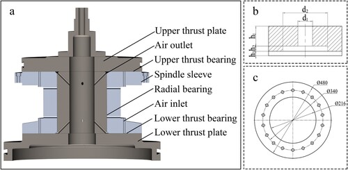
Table 1. Dimensions of the restrictor.

Number per bearing n	Film thickness h3 (µm)	Chamber diameter d2 (mm)	Chamber depth h2 (µm)	Orifice diameter d1 (mm)	Orifice depth h1 (mm)
18	15	8	45	0.2	0.5

The thrust stiffness can be deduced by calculating the axial force when the spindle moves a tiny distance along the axial direction from the stable position, where the axial force is 0. Traditional methods that ignore FSI regard the spindle and spindle sleeve as rigid bodies, as shown in Figure 2(a); this is called the ideal condition in this paper. If external loads and gravity do not exist, the air film thicknesses of the upper and lower thrust bearings will be identical and will be h₃, as shown in Table 1. In this condition, the axial position of the spindle is defined as axial position 0. In the ideal condition, with the spindle at the axial position 0, the ideal upper and lower support forces supporting the spindle, from the upper and lower bearings, respectively, F_i1(0) and F_i2(0), are equal. Hence, the corresponding ideal axial force, F_i(0), is −G, which is less than 0. G is the weight of the spindle. The axial direction from the lower to the upper thrust bearing is defined as the positive direction. Therefore, the spindle has to move in the negative axial direction to a certain axial position z_i0 to achieve stability, which is called the ideal stable position. The ideal axial force, F_i(z_i0), with the spindle at the ideal stable position, is 0, as shown in Equation (1(2) $\{\begin{array}{l}{F}_i(z_{i1})=F_{i1}(z_{i1})-F_{i2}(z_{i1})-G>0\\ F_i(z_{i2})=F_{i1}(z_{i2})-F_{i2}({z_i}_2)-G<0\end{array}$(2) ). F_i1(z_i0) and F_i2(z_i0) represent the ideal upper and lower support forces with the spindle at the axial position z_i0. (1) $F_i(z_{i0})=F_{i1}(z_{i0})-F_{i2}(z_{i0})-G=0$(1) As the spindle moves from the axial position z_i0 along the positive axial direction, the film thickness of the upper thrust bearing increases and the ideal upper support force decreases accordingly. In contrast, the ideal lower support force will increase. Therefore, the ideal axial force will decrease. Similarly, when the spindle moves along the negative axial direction, the ideal axial force will increase. If z_i1 and z_i2 are the adjacent integers of z_i0, and z_i1 is less than z_i2, the ideal axial forces F_i(z_i1) and F_i(z_i2), with the spindle at the axial positions z_i1 and z_i2, will be greater than and less than 0, respectively, as shown in Equation (2(3) $k_{it}=F_i(z_{i1})-F_i(z_{i2})$(3) ). F_i1(z_i1), F_i2(z_i1), F_i1(z_i2) and F_i2(z_i2) represent the ideal upper and lower support forces with the spindle at the axial positions z_i1 and z_i2. (2) $\{\begin{array}{l}{F}_i(z_{i1})=F_{i1}(z_{i1})-F_{i2}(z_{i1})-G>0\\ F_i(z_{i2})=F_{i1}(z_{i2})-F_{i2}({z_i}_2)-G<0\end{array}$(2) Because the distance from the axial position z_i1 to z_i2 is 1 µm, which is small, the ideal thrust stiffness k_it can be regarded as the ratio of the difference between F_i(z_i1) and F_i(z_i2) to the distance from z_i1 to z_i2, as shown in Equation (3(4) $F(z_0)=F_1(z_0)-F_2(z_0)-G=0$(4) ): (3) $k_{it}=F_i(z_{i1})-F_i(z_{i2})$(3) To determine z_i1 and z_i2, and analyze the effect of the axial position of the spindle on the ideal thrust stiffness, the ideal upper and lower support forces, F₁(z) and F₂(z), are calculated separately at 21 axial positions z, which are all integers from −10 µm to 10 µm. With the spindle at the 21 axial positions, the film thicknesses of the thrust bearings are all integers from 5 µm to 25 µm. Besides, because the two thrust bearings are identical, only the support forces of the bearings with the 21 film thicknesses need to be calculated to deduce the ideal thrust stiffness.

Figure 2. Schematic diagram of the phenomenon of fluid–structure interaction (FSI).

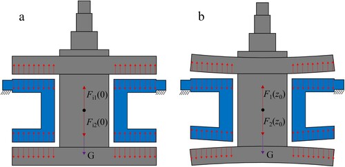
The proposed steady two-way FSI modeling method considers the phenomenon of FSI, as shown in Figure 2(b), which is called the actual condition in this paper. As in the ideal condition, the spindle has to move a certain distance z₀ along the axial direction to be stable in the actual condition and, accordingly, the actual axial force F(z₀) is 0, as shown in Equation (4(5) $\{\begin{array}{l}F(z_1)=F_1(z_1)-F_2(z_1)-G>0\\ F(z_2)=F_1(z_2)-F_2(z_2)-G<0\end{array}$(5) ). F₁(z₀) and F₂(z₀) represent the actual upper and lower support forces with the spindle at the axial position z₀. (4) $F(z_0)=F_1(z_0)-F_2(z_0)-G=0$(4) If z₁ and z₂ are the adjacent integers of z₀, and z₁ is less than z₂, then, as in Equation (2(3) $k_{it}=F_i(z_{i1})-F_i(z_{i2})$(3) ), the actual axial forces F(z₁) and F(z₂), with the spindle at axial positions z₁ and z₂, will be greater than and less than 0, respectively, as shown in Equation (5(6) $k_t=F(z_1)-F(z_2)$(6) ). F₁(z₁), F₂(z₁), F₁(z₂) and F₂(z₂) represent the actual upper and lower support forces with the spindle at the axial positions z₁ and z₂. (5) $\{\begin{array}{l}F(z_1)=F_1(z_1)-F_2(z_1)-G>0\\ F(z_2)=F_1(z_2)-F_2(z_2)-G<0\end{array}$(5) Similarly, the actual thrust stiffness k_t can be regarded as the ratio of the difference value between F(z₁) and F(z₂) to the distance from z₁ to z₂, as shown in Equation (6(7) $\{\begin{array}{l}{k}_{it}(h)=F_{i{z}_{i1}}(h)-F_{i{z}_{i2}}(h)\\ F_{i{z}_{i1}}(h)=F_i(h+z_{i1})-F_i(h-z_{i1})-G>0\\ F_{i{z}_{i2}}(h)=F_i(h+z_{i2})-F_i(h-z_{i2})-G<0\end{array}$(7) ): (6) $k_t=F(z_1)-F(z_2)$(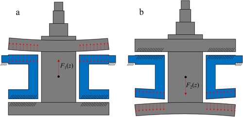6) To determine z₁ and z₂, and analyze the effect of the axial position of the spindle on the actual thrust stiffness, the actual upper and lower support forces, F₁(z) and F₂(z), are also calculated separately at 21 axial positions z, which are all integers from −10 µm to 10 µm. First, the assembly of the spindle system, consisting of the spindle and spindle sleeve, at a certain axial position z, is built. The FSI model used to calculate F₁(z) is composed of a static model of the assembly and a CFD model of the upper bearing. To consider the solid deformations of the upper thrust plate and spindle, the two support surfaces of the lower bearing are fixed, as shown in Figure 3(a). The two support surfaces of the upper bearing from the static model are coupled with those from the CFD model. In one iteration, the solid deformations of the support surfaces calculated from the static model are transferred to update the mesh in the CFD model. The support forces from the support surfaces calculated from the CFD model are transmitted to update the support forces applied to deform the support surfaces in the static model. Similarly, the FSI model used to calculate F₂(z) consists of a static model of the assembly and a CFD model of the lower bearing. In the static model, the two support surfaces of the upper bearing are fixed and the two support surfaces of the lower bearing are coupled with those from the CFD model, as shown in Figure 3(b).

Figure 3. Schematic diagram of the fluid–structure interaction (FSI) models to calculate F₁(z) and F₂(z).

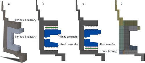
Both the solid structures of the spindle system and the thrust bearings are axially symmetrical. To reduce calculation costs, just 1/18 of the spindle system is modeled, and the support force of the bearing can be gained as the support force calculated from the model multiplied by 18. The solid structures are built as shown in Figure 4(a). The sections of the solid structures are imposed with periodic boundaries. The rest of the constraints in the static models used to calculate F₁(z) and F₂(z) are shown in Figure 4(b) and (c), respectively. Because the CFD mesh has to be dense to guarantee good calculation accuracy, the solid mesh is refined to decrease interpolation errors in the process of data transfer, as shown in Figure 4(d).

Figure 4. Static models of the fluid–structure interaction (FSI) models.

Because the upper and lower bearings are identical, their CFD models are constructed uniformly, as shown in Figure 5. The boundary conditions of the CFD model are shown in Figure 5(a). In the figure, several structural sizes of the thrust bearing are amplified to show the boundary conditions clearly. The inlet is set as the pressure inlet and the supply pressure is 0.5 MPa (gauge pressure). The bearing outlet is set as the pressure outlet and the discharge pressure is 0 (gauge pressure). The sections of the CFD model are also set as periodic boundaries. To enhance the convergence rate and calculation accuracy, a structured hexahedral mesh is generated, as shown in Figure 5(b).

Figure 5. Computational fluid dynamics (CFD) models of the fluid–structure interaction (FSI) models.

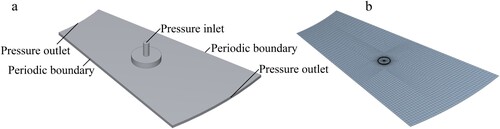
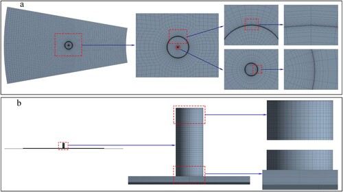
Figure 6 illustrates the details of the CFD mesh. Because the air flow in the field of the air film has a low Reynolds number, the first layer mesh of the air film is generated in the viscous sublayer. Therefore, enhanced wall functions are used to simulate the flow field near the wall surfaces. To guarantee good calculation accuracy, a finer grid scheme in the boundary layer of all wall surfaces must be used to ensure that their first layers are in the viscous sublayer. To avoid calculation errors derived from the large dimensional change of the adjacent mesh, all variation factors of the adjacent mesh are controlled to be less than 1.3. The CFD mesh details of the support surfaces, the ring surface of the chamber and the inlet are shown in Figure 6(a). Given the large structural changes in the orifice inlet and the transition position between the orifice and the chamber, the mesh in the two regions is refined to simulate the flow field accurately. To ensure that the first mesh of the two support surfaces and the chamber ring surface is in the viscous sublayer, and that the CFD mesh has adequate density to simulate the flow field accurately, the mesh layers of the air film and chamber are 25 and 20, respectively, in the thickness direction. The CFD mesh details in the thickness direction are shown in Figure 6(b).

Figure 6. Mesh details of the computational fluid dynamics (CFD) model.

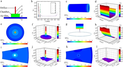
To verify that all of the first layer of the near-wall mesh is in the viscous sublayer, the Y⁺ of all wall surfaces is analyzed when the ideal and actual thrust stiffnesses are calculated. Y⁺ of all the wall surfaces, when the ideal support force F_i1(0) is calculated, is shown in Figure 7. Figure 7(a) is the schematic diagram of all wall surfaces of the thrust bearing. Figure 7(b) is the scatter diagram of Y⁺ of the nodes on the five wall surfaces, where the abscissa is the axial coordinates of all nodes on the surfaces. Figure 7(c), (e), (g), (i) and (k) are the contours of Y⁺ of the five surfaces, 1, 2, 3, 4 and 5, respectively. Because the axial coordinates z of all nodes on any of the wall surfaces 2, 4 and 5 are identical, the three-dimensional surface diagrams of Y⁺ under x and y coordinates of the nodes on the three surfaces can be drawn, as shown in Figure 7(f), (j) and (l), respectively. The Cartesian coordinates x and y of the nodes on the two surfaces 1 and 3 are converted to cylindrical coordinates θ and r. Because the radii r of all nodes on any of the two wall surfaces are identical, the three-dimensional surface diagrams of Y⁺ under θ and z coordinates of the nodes on the two surfaces can be drawn, as shown in Figure 7(d) and (h), respectively. It can be seen that all Y⁺ values are less than 2.5 and almost all Y⁺ values are less than 1.

Figure 7. Y⁺ of the wall surfaces with the ideal thrust stiffness calculated.

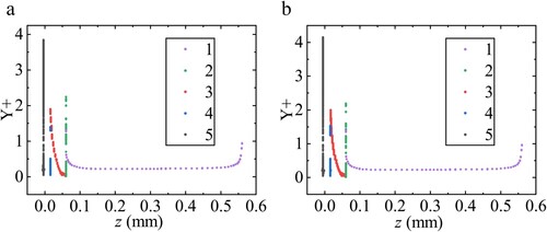
The scatter diagrams of Y⁺ of the nodes on the five wall surfaces when the actual upper and lower support forces F₁(0) and F₂(0), with the spindle at the axial position 0, are calculated as shown in Figure 8. Figure 8(a) and (b) illustrate Y⁺ of the wall surfaces when F₁(0) and F₂(0), respectively, are calculated. It can be seen that all Y⁺ values are less than 4.5 and almost all Y⁺ values are less than 1. Therefore, the near wall mesh of all wall surfaces meets the requirements.

Figure 8. Y⁺ of the wall surfaces with the actual thrust stiffness calculated.

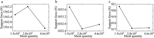
In the CFD model, the RNG k-ϵ turbulence model is used to simulate the turbulent flow in the bearing accurately. Owing to the great pressure change in the bearing, the compressibility of air is considered. Because the calculation results are related to mesh density, the mesh independency test is conducted to guarantee that the current mesh quantity is adequate. Sparser and denser meshes are obtained by refining and rarefying the current mesh. The quantities of sparser, current and denser mesh are 152,000, 282,000 and 459,000, respectively. Because the support forces are the objective calculation results used to deduce the thrust stiffness, F_i1(0), F₁(0) and F₂(0) under the three mesh quantities are calculated, as shown in Figure 9(a)–(c), respectively. Because all errors of the three support forces calculated with the sparse and current mesh are less than 0.4%, taking the calculation results with the denser mesh as the reference, the current mesh quantity is adequate for the CFD model.

Figure 9. Ideal support force and actual upper and lower support forces under three mesh densities.

3. Results and discussion

3.1. Solid deformations

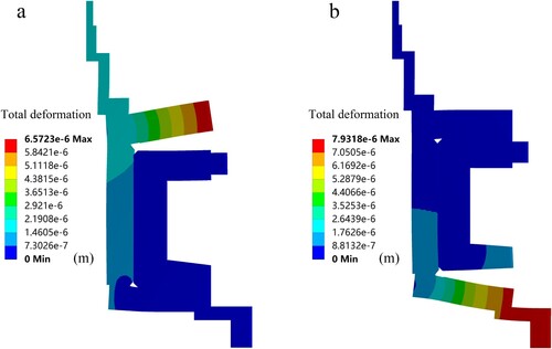
The calculation results of the FSI models with the spindle at the axial position 0 are taken as an example to study solid deformations, as shown in Figure 10. Figure 10(a) and (b) illustrate the solid deformations when F₁(0) and F₂(0), respectively, are calculated. It can be seen that both the upper and lower thrust plates have a large deformation. Their maximum deformations are 6.6 µm and 7.9 µm, which are 44% and 53% of the air film thickness, respectively.

Figure 10. Contours of the solid deformations.

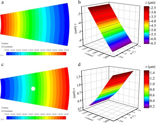
Because the sizes of the support surfaces are large, the small change in the radial coordinates of nodes on the support surfaces hardly deforms the bearing structure, which can be ignored. Nevertheless, the small change in the z coordinates of the nodes can deform the bearing structure a lot, because the air film thickness is thin. Therefore, the change in the z coordinates of the nodes is the major factor that transforms the bearing structure and thus affects the performance. Figure 11 illustrates the variation in the z coordinates of nodes on the two support surfaces of the upper bearing. The contours on the support surfaces of the spindle and spindle sleeve are shown in Figure 11(a) and (c), respectively. The Cartesian coordinates of nodes on the two support surfaces are converted to polar coordinates to draw the three-dimensional surface diagrams of the variations in z, as shown in Figure 11(b) and (d), respectively. Similarly, the contours of the variations in the z coordinates of nodes on the two support surfaces of the lower bearing are shown in Figure 12(a) and (c). The three-dimensional surface diagrams of the variations in z are shown in Figure 12(b) and (d), respectively.

Figure 11. Variations in z of the upper bearing.

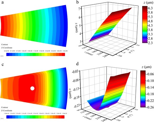
Figure 12. Variations in z of the lower bearing.

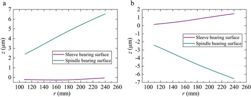
It can be seen from Figures 11 and 12 that the z coordinates of the nodes on any support surface, which have different polar angles and the same polar radius, are almost identical. The variations in z under different polar radii are shown in Figure 13, with the polar angle at 0. Figure 13(a) illustrates the variations in z of the two support surfaces of the upper bearing. It can be seen that the shape of the cross-section of the upper bearing changes from rectangular to right trapezoid, because the variations in z on the support surface from the spindle sleeve can be ignored compared with those from the spindle. Figure 13(b) illustrates the variations in z on the support surfaces of the lower bearing. The shape of the cross-section of the lower bearing can be regarded as a trapezoid.

Figure 13. Variations in z of the upper and lower bearings in the section.

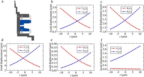
To analyze the effect of the axial position z on solid deformations, 10 points in the cross-section with the polar angle at 0 are chosen, as shown in Figure 14(a). The points, B₁, C₁, D₁ and E₁ are the vertices of the cross-section of the upper bearing, and B₂, C₂, D₂ and E₂ are those of the lower bearing. Figure 14(b)–(f) illustrates the variations in the z coordinates of the 10 points with the spindle at different axial positions. It can be seen that the variations in the z coordinates of the five points of the upper bearing decrease, but those of the five points of the lower bearing increase with the increase in the axial position of the spindle z. That is, the upper solid deformation becomes smaller and the lower solid deformation becomes larger as the spindle moves along the positive axial direction.

Figure 14. Variations in z of 10 points under different axial positions.

3.2. Pressure distribution

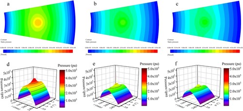
Because of the great structural deformations of the two bearings, the actual inner flow field and support forces will change a lot compared to the ideal condition. The ideal pressure contour of the support surface and the actual pressure contours of the upper and lower support surfaces are shown in Figure 15(a)–(c), respectively. The three-dimensional surface diagrams of pressure under the polar coordinates of the support surfaces are shown in Figure 15(d)–(f), respectively. It can be seen that the actual pressure distribution of the upper support surface is greater than that of the lower support surface, but is less than the ideal pressure distribution.

Figure 15. Ideal and actual pressure distributions of the support surfaces.

3.3. Effect of the axial position

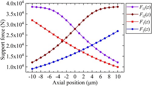
Figure 16 illustrates the ideal and actual upper and lower support forces with the spindle at different axial positions z from −10 µm to 10 µm. It can be seen that the ideal upper and lower support forces F_i1(z) and F_i2(z) are greater than the actual upper and lower support forces F₁(z) and F₂(z), respectively. With the increase in z, the air film thickness of the upper bearing increases and that of the lower bearing decreases. Hence, the ideal and actual upper support forces F_i1(z) and F₁(z) decrease, and the ideal and actual lower support forces F_i2(z) and F₂(z) increase with the increase in z.

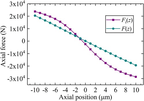
Figure 16. Ideal and actual upper and lower support forces under different axial positions.

The ideal axial force F_i(z) can be obtained by subtracting F_i2(z) and gravity from F_i1(z), and the actual axial force F(z) can be obtained by subtracting F₂(z) and gravity from F₁(z), as shown in Figure 17. It can be seen that both F_i(z) and F(z) decrease with the increase in z. F_i(0) is −2421.58 N, which is less than 0, and F_i(−1) is 1704.92 N, which is greater than 0, so z_i1 is −1 µm and z_i2 is 0. The ideal thrust stiffness k_it can be deduced as 4126.50 N/µm by Equation (3(4) $F(z_0)=F_1(z_0)-F_2(z_0)-G=0$(4) ). Similarly, because F(0) is 158.96 N and F(1) is −1884.50 N, z₁ is 0 and z₂ is 1 µm. The actual thrust stiffness k_t is 2043.46 N/µm, based on Equation (6(7) $\{\begin{array}{l}{k}_{it}(h)=F_{i{z}_{i1}}(h)-F_{i{z}_{i2}}(h)\\ F_{i{z}_{i1}}(h)=F_i(h+z_{i1})-F_i(h-z_{i1})-G>0\\ F_{i{z}_{i2}}(h)=F_i(h+z_{i2})-F_i(h-z_{i2})-G<0\end{array}$(7) ), which is obviously less than k_it. Therefore, the phenomenon of FSI greatly decreases the thrust stiffness of the spindle.

Figure 17. Ideal and actual axial forces under different axial positions.

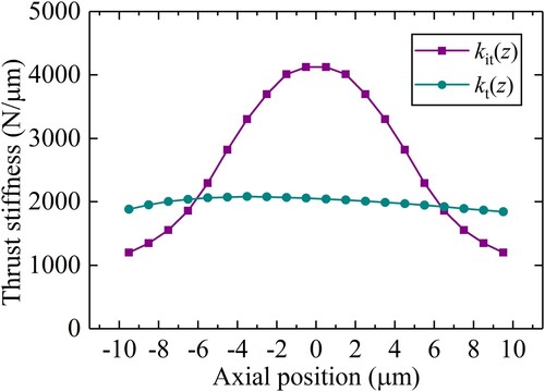
The ideal and actual thrust stiffnesses, k_it(z) and k_t(z), when the spindle is at the axial position of z, can be regarded as the difference of F_i(z) and F(z), respectively, as shown in Figure 18. It can be seen that k_it(z) is symmetrical about the vertical line z = 0. In other words, the ideal thrust stiffnesses k_it(z) and k_it(−z), when the spindle is at the axial positions of z and −z, are identical. As the spindle moves from the axial position 0 along the positive or negative axial direction, k_it(z) decreases. Although k_t(z) increases and then decreases with the increase in z, which is similar to k_it(z), the amplitude of the variation in k_t(z) is less than that of k_it(z). In other words, the existence of FSI notably decreases the effect of the axial position of the spindle on the thrust stiffness.

Figure 18. Ideal and actual thrust stiffness under different axial positions.

3.4. Effect of the air film thickness

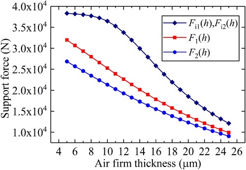
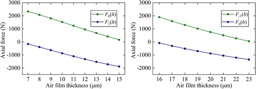
As a key design parameter, the air film thickness h has an important effect on the thrust stiffness, which can also be studied using the data of the support forces with the spindle at different axial positions z. The air film thickness of the upper thrust bearing h₁ is 15 µm plus the axial position z, and that of the lower thrust bearing h₂ is 15 µm minus z. Therefore, h₁ and h₂ can be any integer from 5 µm to 25 µm, because positions z are all integers from −10 µm to 10 µm. The ideal and actual upper and lower support forces F_i1(h), F_i2(h), F₁(h) and F₂(h) under different h from 5 µm to 25 µm can be obtained from the data in Figure 16, as shown in Figure 19. It can be seen that all of these forces decrease with the increase in h. Under the effect of FSI, both F₁(h) and F₂(h) are obviously less than F_i1(h).

Figure 19. Ideal and actual upper and lower support forces under different air film thicknesses.

As in Equations (2(3) $k_{it}=F_i(z_{i1})-F_i(z_{i2})$(3) ) and (3(4) $F(z_0)=F_1(z_0)-F_2(z_0)-G=0$(4) ), the ideal thrust stiffness with the air film thickness of h, k_it(h), can be deduced by Equation (7(8) $\{\begin{array}{l}{k}_t(h)=F_{z_1}(h)-F_{z_2}(h)\\ F_{z_1}(h)=F_1(h+z_1)-F_2(h-z_1)-G>0\\ F_{z_2}(h)=F_1(h+z_2)-F_2(h-z_2)-G<0\end{array}$(8) ). F_izi1(h) and F_izi2(h) represent the ideal axial forces with the spindle at the axial positions z_i1 and z_i2. F_i(h + z_i1), F_i(h + z_i2), F_i(h − z_i1) and F_i(h − z_i2) are the ideal support forces with the air film thicknesses of h + z_i1, h + z_i2, h − z_i1 and h − z_i2, respectively. Therefore, k_it(h) can be acquired by determining the two axial positions, z_i1 and z_i2. As the spindle is at the axial position 0, the ideal axial force F_i0(h) is −G, which is less than 0. Hence, the ideal stable position z_i0 must be less than 0. For a certain air film thickness h, the ideal axial force F_i–1(h), with the spindle at the axial position −1 µm, is calculated. If F_i–1(h) is greater than 0, z_i1 is −1 µm and z_i2 is 0. Or, one can continue to calculate the ideal axial force F_i–2(h) until F_izi1(h) greater than 0 emerges, and z_i2 is equal to z_i1 plus 1. In this way, z_i1 and z_i2 under different film thicknesses can be found. If the air film thicknesses h are 9 µm and 10 µm, z_i1 is −2 µm and z_i2 is −1 µm; if the air film thicknesses h are all integers from 11 µm to 23 µm, z_i1 is −1 µm and z_i2 is 0. (7) $\{\begin{array}{l}{k}_{it}(h)=F_{i{z}_{i1}}(h)-F_{i{z}_{i2}}(h)\\ F_{i{z}_{i1}}(h)=F_i(h+z_{i1})-F_i(h-z_{i1})-G>0\\ F_{i{z}_{i2}}(h)=F_i(h+z_{i2})-F_i(h-z_{i2})-G<0\end{array}$(7) Similarly, as in Equations (5(6) $k_t=F(z_1)-F(z_2)$(6) ) and (6(7) $\{\begin{array}{l}{k}_{it}(h)=F_{i{z}_{i1}}(h)-F_{i{z}_{i2}}(h)\\ F_{i{z}_{i1}}(h)=F_i(h+z_{i1})-F_i(h-z_{i1})-G>0\\ F_{i{z}_{i2}}(h)=F_i(h+z_{i2})-F_i(h-z_{i2})-G<0\end{array}$(7) ), the actual thrust stiffness with the air film thickness of h, k_t(h), can be deduced by Equation (8). F_z1(h) and F_z2(h) are the actual support forces with the spindle at the axial positions of z₁ and z₂. F₁(h + z₁) and F₁(h + z₂) are the actual upper support forces with the air film thicknesses of h + z₁ and h + z₂, respectively; F₂(h − z₁) and F₂(h − z₂) are the actual lower support forces with the air film thicknesses of h − z₁ and h − z₂, respectively. (8) $\{\begin{array}{l}{k}_t(h)=F_{z_1}(h)-F_{z_2}(h)\\ F_{z_1}(h)=F_1(h+z_1)-F_2(h-z_1)-G>0\\ F_{z_2}(h)=F_1(h+z_2)-F_2(h-z_2)-G<0\end{array}$(8) The actual stable positions z₀ are not the same for different air film thicknesses h. The method used to determine F_z1(h) and F_z2(h) is shown in Figure 20, by which k_t(h) can be deduced. First, the actual axial force F₀(h) with the spindle at the axial position 0 is calculated for a certain air film thickness h. If F₀(h) is greater than 0, F₁(h) is calculated. Then, if F₁(h) is greater than 0, F₂(h) is calculated, and so on, until F_z2(h) that is less than 0 emerges, and z₁ is equal to z₂ minus 1. On the contrary, if F₀(h) is less than 0, F₋₁(h) is calculated. Then, if F₋₁(h) is less than 0, F₋₂(h) is calculated, and so on, until F_z1(h) that is greater than 0 emerges, and z₂ is equal to z₁ plus 1. Then, z₁ and z₂ under different air film thicknesses h can be obtained.

Figure 20. Method to find F_z1(h) and F_z2(h).

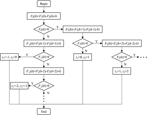
If the air film thicknesses h are all integers from 7 µm to 15 µm, z₁ is 0 and z₂ is 1 µm; if the air film thicknesses h are all integers from 16 µm to 23 µm, z₁ is −1 µm and z₂ is 0. F_z1(h) and F_z2(h) under different air film thicknesses h are shown in Figure 21.

Figure 21. F_z1(h) and F_z2(h) under different air film thicknesses h.

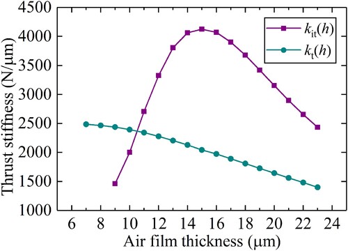
The ideal and actual thrust stiffnesses, k_it(h) and k_t(h), under different air film thicknesses can be deduced by Equations (7(8) $\{\begin{array}{l}{k}_t(h)=F_{z_1}(h)-F_{z_2}(h)\\ F_{z_1}(h)=F_1(h+z_1)-F_2(h-z_1)-G>0\\ F_{z_2}(h)=F_1(h+z_2)-F_2(h-z_2)-G<0\end{array}$(8) ) and (8), as shown in Figure 22. It can be seen that both k_it(h) and k_t(h) increase and then decrease with the increase in h, but the amplitude of the variation in k_it(h) is greater than that of k_t(h). Besides, their extreme points are different. The extreme point of k_it(h) is 15 µm, which is the designed value, and that of k_t(h) is 7 µm. It can be seen that the film thickness of 15 µm is not the best one to obtain the maximum thrust stiffness compared with 7 µm, based on the proposed method. Therefore, the phenomenon of FSI changes considerably the effect of h on the thrust stiffness.

Figure 22. Ideal and actual thrust stiffness under different air film thicknesses.

4. Experimental verification

The thrust stiffness of the aerostatic spindle was measured in the experimental facility shown in Figure 23(a) (Gao et al., 2017). A capacitance micrometer was used to measure the axial displacement of the spindle under the loads of two mass blocks that were hung symmetrically on the two tool holders. The experimental data are shown in Table 2. The scatter diagram of the data and the fitting straight line are shown in Figure 23(b). The gradient of the fitting straight line is 2224.9 N/µm, which can be regarded as the tested thrust stiffness. The thrust stiffness based on the proposed steady two-way FSI modeling method is 2043.46 N/µm. Therefore, the calculation error of the proposed steady method is 8.15%, which mainly stems from the experimental error, and the effects of the assembly error and the bearing surface quality, which are not considered in the FSI models. The thrust stiffness based on the traditional method that does not consider solid deformations is 4126.50 N/µm. Therefore, the calculation error without considering FSI is 85.47%, which is much greater than that based on the proposed steady method. It can be seen that the proposed steady method has good accuracy for studying the thrust stiffness of the static pressure spindle when the phenomenon of FSI is noticeable, and is more reliable than the traditional method, which ignores the effects of FSI.

Figure 23. Experimental facility and data.

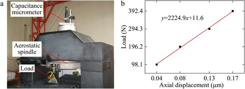
Table 2. Experimental data.

Load (kg)	10	20	30	40
Axial displacement (µm)	0.04	0.08	0.13	0.17

5. Conclusions

This paper proposes a steady two-way FSI modeling method to study the effect of FSI on the thrust stiffness of an aerostatic spindle. The main conclusions are as follows.

1. The maximum solid deformation under support forces is 7.9 µm, which is about 53% of the air film thickness. The sectional shape of the bearing becomes trapezoid owing to the solid deformation.

2. Both the ideal and actual thrust stiffnesses, k_it(z) and k_t(z), increase and then decrease with the increase in the axial position of spindle z. The amplitude of the variation in k_t(z) is less than that of k_it(z) with the increase in z.

3. Both the ideal and actual thrust stiffnesses, k_it(h) and k_t(h), increase and then decrease with the increase in the air film thickness h. The extreme point of k_it(h) is 15 µm, which is the designed value, and that of k_t(h) is 7 µm.

4. The proposed method is verified as reliable by the experimental results. The calculation error of the proposed steady method is 8.15%, which is much less than that based on the traditional method ignoring FSI.

The calculation time can be greatly shortened based on the proposed method instead of the transient method, when the performance of a static pressure spindle or slide is studied with consideration of FSI. However, the proposed method still needs a long design cycle, as a static pressure spindle or slide with high load-carrying capacity and stiffness is being designed. Future research could focus on finding a more efficient method to study the phenomenon of FSI.

Disclosure statement

No potential conflict of interest was reported by the authors.

Additional information

Funding

The authors gratefully acknowledge the financial support from the National Natural Science Foundation of China (52105439) and the Postdoctoral Foundation of Hei Long Jiang Province [grant number LBH-Z19149].

References

- Aguirre, G., Al-Bender, F., & Van Brussel, H. (2010). A multiphysics model for optimizing the design of active aerostatic thrust bearings. Precision Engineering, 34(3), 507–515. https://doi.org/10.1016/j.precisioneng.2010.01.004
- An, C. H., Zhang, Y., Xu, Q., Zhang, F. H., Zhang, J. F., Zhang, L. J., & Wang, J. H. (2010). Modeling of dynamic characteristic of the aerostatic bearing spindle in an ultra-precision fly cutting machine. International Journal of Machine Tools and Manufacture, 50(4), 374–385. https://doi.org/10.1016/j.ijmachtools.2009.11.003
- Chen, W., Liang, Y., Sun, Y., Huo, D., Lu, L., & Liu, H. (2014). Design philosophy of an ultra-precision fly cutting machine tool for KDP crystal machining and its implementation on the structure design. The International Journal of Advanced Manufacturing Technology, 70(1–4), 429–438. https://doi.org/10.1007/s00170-013-5299-9
- Chen, Y. S., Chiu, C. C., & Cheng, Y. D. (2010). Influences of operational conditions and geometric parameters on the stiffness of aerostatic journal bearings. Precision Engineering, 34(4), 722–734. https://doi.org/10.1016/j.precisioneng.2010.04.001
- Eleshaky, M. E. (2009). CFD investigation of pressure depressions in aerostatic circular thrust bearings. Tribology International, 42(7), 1108–1117. https://doi.org/10.1016/j.triboint.2009.03.011
- Fillon, M., Wodtke, M., & Wasilczuk, M. (2015). Effect of presence of lifting pocket on the THD performance of a large tilting-pad thrust bearing. Friction, 3(4), 266–274. https://doi.org/10.1007/s40544-015-0092-4
- Gao, Q., Chen, W., Lu, L., Huo, D., & Cheng, K. (2019). Aerostatic bearings design and analysis with the application to precision engineering: State-of-the-art and future perspectives. Tribology International, 135(February), 1–17. https://doi.org/10.1016/j.triboint.2019.02.020.
- Gao, Q., Lu, L., Chen, W., Chen, G., & Wang, G. (2017). A novel modeling method to investigate the performance of aerostatic spindle considering the fluid-structure interaction. Tribology International, 115(April), 461–469. https://doi.org/10.1016/j.triboint.2017.06.016
- Ghalandari, M., Bornassi, S., Shamshirband, S., Mosavi, A., & Chau, K. W. (2019). Investigation of submerged structures’ flexibility on sloshing frequency using a boundary element method and finite element analysis. Engineering Applications of Computational Fluid Mechanics, 13(1), 519–528. https://doi.org/10.1080/19942060.2019.1619197
- Haynam, C. A., Wegner, P. J., Auerbach, J. M., Bowers, M. W., Dixit, S. N., Erbert, G. V., Heestand, G. M., Henesian, M. A., Hermann, M. R., Jancaitis, K. S., Manes, K. R., Marshall, C. D., Mehta, N. C., Menapace, J., Moses, E., Murray, J. R., Nostrand, M. C., Orth, C. D., Patterson, R., … Van Wonterghem, B. M. (2007). National ignition facility laser performance status. Applied Optics, 46(16), 3276–3303. https://doi.org/10.1364/AO.46.003276
- Hogan, W. J., Moses, E. I., Warner, B. E., Sorem, M. S., & Soures, J. M. (2001). The national ignition facility. Nuclear Fusion, 41(5), 567–573. https://doi.org/10.1088/0029-5515/41/5/309
- Huang, S., Su, X., & Qiu, G. (2015). Transient numerical simulation for solid-liquid flow in a centrifugal pump by DEM-CFD coupling. Engineering Applications of Computational Fluid Mechanics, 9(1), 411–418. https://doi.org/10.1080/19942060.2015.1048619
- Jiang, J., Cai, H., Ma, C., Qian, Z., Chen, K., & Wu, P. (2018). A ship propeller design methodology of multi-objective optimization considering fluid–structure interaction. Engineering Applications of Computational Fluid Mechanics, 12(1), 28–40. https://doi.org/10.1080/19942060.2017.1335653
- Lee, W. B., & Cheung, C. F. (2001). A dynamic surface topography model for the prediction of nano-surface generation in ultra-precision machining. International Journal of Mechanical Sciences, 43(4), 961–991. https://doi.org/10.1016/S0020-7403(00)00050-3
- Lu, L., Gao, Q., Chen, W., Liu, L., & Wang, G. (2017). Investigation on the fluid–structure interaction effect of an aerostatic spindle and the influence of structural dimensions on its performance. Proceedings of the Institution of Mechanical Engineers, Part J: Journal of Engineering Tribology, 231(11), 1434–1440. https://doi.org/10.1177/1350650117697826
- Norton, M. A., Adams, J. J., Carr, C. W., Donohue, E. E., Feit, M. D., Hackel, R. P., Hollingsworth, W. G., Jarboe, J. A., Matthews, M. J., Rubenchik, A. M., & Spaeth, M. L. (2007). Growth of laser damage in fused silica: Diameter to depth ratio. Laser-Induced Damage in Optical Materials, 2007(6720), 67200H. https://doi.org/10.1117/12.748441
- Novotný, P., Hrabovský, J., Juračka, J., Klíma, J., & Hort, V. (2019). Effective thrust bearing model for simulations of transient rotor dynamics. International Journal of Mechanical Sciences, 157-158(December 2018), 374–383. https://doi.org/10.1016/j.ijmecsci.2019.04.057
- Salih, S. Q., Aldlemy, M. S., Rasani, M. R., Ariffin, A. K., Ya, T. M. Y. S. T., Al-Ansari, N., Yaseen, Z. M., & Chau, K. W. (2019). Thin and sharp edges bodies-fluid interaction simulation using cut-cell immersed boundary method. Engineering Applications of Computational Fluid Mechanics, 13(1), 860–877. https://doi.org/10.1080/19942060.2019.1652209
- Shi, J., Cao, H., & Jin, X. (2019). Investigation on the static and dynamic characteristics of 3-DOF aerostatic thrust bearings with orifice restrictor. Tribology International, 138(June), 435–449. https://doi.org/10.1016/j.triboint.2019.06.026
- Spentzos, A., Barakos, G. N., Badcock, K. J., Richards, B. E., Coton, F. N., Galbraith, R. A. M. D., Berton, E., & Favier, D. (2007). Computational fluid dynamics study of three-dimensional dynamic stall of various planform shapes. Journal of Aircraft, 44(4), 1118–1128. https://doi.org/10.2514/1.24331
- Wang, Z., Zha, J., Chen, Y., & Zhao, W. (2014). Influencing of fluid-structure interactions on static and dynamic characteristics of oil hydrostatic guideways. Journal of Mechanical Engineering, 50(9), 148–152. https://doi.org/10.3901/JME.2014.09.148
- Wu, Q., Sun, Y., Chen, W., Liu, H., & Luo, X. (2019). An mechatronics coupling design approach for aerostatic bearing spindles. International Journal of Precision Engineering and Manufacturing, 20(7), 1185–1196. https://doi.org/10.1007/s12541-019-00098-w
- Yang, H., Cheng, J., Liu, Z., Liu, Q., Zhao, L., Wang, J., & Chen, M. (2020). Dynamic behavior modeling of laser-induced damage initiated by surface defects on KDP crystals under nanosecond laser irradiation. Scientific Reports, 10(1), 1–11. https://doi.org/10.1038/s41598-019-56847-4
- Yifei, L., Yihui, Y., Hong, Y., Xinen, L., Jun, M., & Hailong, C. (2017). Modeling for optimization of circular flat pad aerostatic bearing with a single central orifice-type restrictor based on CFD simulation. Tribology International, 109(December 2016), 206–216. https://doi.org/10.1016/j.triboint.2016.12.044
- Yu, X., Wang, Y., Zhou, D., Wu, G., Zhou, W., & Bi, H. (2019). Heat transfer characteristics of high speed and heavy load hydrostatic bearing. IEEE Access, 7, 110770–110780. https://doi.org/10.1109/ACCESS.2019.2933471
- Zeng, C., Wang, W., Cheng, X., Zhao, R., & Cui, H. (2021). Three-dimensional flow state analysis of microstructures of porous graphite restrictor in aerostatic bearings. Tribology International, 159(December 2020), 106955. https://doi.org/10.1016/j.triboint.2021.106955
- Zhang, S. J., To, S., Zhang, G. Q., & Zhu, Z. W. (2015). A review of machine-tool vibration and its influence upon surface generation in ultra-precision machining. International Journal of Machine Tools and Manufacture, 91, 34–42. https://doi.org/10.1016/j.ijmachtools.2015.01.005
- Zhang, S. J., To, S., Zhu, Z. W., & Zhang, G. Q. (2016). A review of fly cutting applied to surface generation in ultra-precision machining. International Journal of Machine Tools and Manufacture, 103, 13–27. https://doi.org/10.1016/j.ijmachtools.2016.01.001
- Zhang, Y., Lu, C., Zhao, H., Shi, W., & Liang, P. (2019). Error averaging effect of hydrostatic journal bearings considering the influences of shaft rotating speed and external load. IEEE Access, 7, 106346–106358. https://doi.org/10.1109/ACCESS.2019.2931948