Effects of pulsed endwall air injection on corner separation and vortical flow of a compressor cascade

ABSTRACT

Air injection is an effective method to eliminate flow separation and improve blade loading in compressors. In existing studies on unsteady air injection, achieving a better control effect than steady injection with lower injection consumption is a major difficulty and challenge. In this work, pulsed endwall air injection (PEAI) was carried out numerically in a highly loaded compressor cascade under different injection frequencies and injection amplitudes. The mechanism through which PEAI influences corner separation and vortical flow, especially the effect of initial injection phase on the flow field of compressor cascade, was revealed. The results showed that PEAI effectively suppressed the corner separation with lower injection mass flow rate compared with steady endwall air injection (SEAI). The time-averaged overall loss coefficient and endwall loss coefficient were reduced by 10.5% and 28.7%, respectively, under the optimal PEAI scheme. Higher injection amplitude exhibited a more effectively controlled range in the suction corner, which led to a decrease in corner separation and deterioration of the mid-span flow field. The interaction between trailing edge separation and low-momentum fluid at mid-span led to the formation of an injection vortex. When conducting PEAI, the effect of inertia was observed for flow in the injection hole, which was derived from the interactions between injection fluid at different velocities and will increase with the improvement of injection frequency. The effects of injection location and diameter of the injection hole were also investigated. The injection location of PEAI affected the flow field by changing the effect region of the injection and low-momentum fluid near the endwall. The injection hole diameter had a significant impact on the intensity of the passage vortex and mid-span flow field.

Keywords:

• Pulsed endwall air injection
• compressor
• corner separation
• flow control
• vortex

1. Introduction

The requirements of higher thrust weight ratio and efficiency of modern aero-engines entail the increasing of blade loading of axial compressors (Bullock & Johnsen, 1965; Wennerstrom, 1990). However, in highly loaded compressors, flow separations, especially three-dimensional (3D) corner separation, inevitably occur, which will limit the improvement of compressor blade loading (Bryce et al., 1995; Gbabebo et al., 2005).

To control flow separations in axial compressors, researchers have been working on developing flow control technologies (both passive flow control methods and active flow control methods) for almost a century (Culley et al., 2004; Kan et al., 2020; Tang et al., 2019). The passive flow control method has been widely used in compressors because of its low cost and simple structure, and the optimization algorithms developed in recent years have further improved its control effect (Ghalandari et al., 2019). Compared with the inherent weakness of passive flow control methods, i.e. the control effect will weaken under off-design conditions (Rivir et al., 2000), active flow control methods, such as air injection (Culley et al., 2004), boundary layer suction (Sun et al., 2021) and plasma actuator (Zhang et al., 2019), can well adapt to a wider range of operating condition of compressors, which attracts much more attention from researchers. In addition, with the development of computational fluid dynamics (CFD), the accuracy in simulating the ability to capture the flow field has been significantly improved, which has effectively decreased the difficulty of active flow control methods in experiments (Salih et al., 2019).

Among the active control methods, air injection has been proved to be able to suppress flow separations in compressors effectively (Brück et al., 2016; Culley et al., 2004; Sarimurat & Dang, 2014). The existing literature (Evans et al., 2012; Zheng et al., 2005) on air injection has proved that air injection can re-energize the low-momentum fluid in the boundary layer, which suppresses or eliminates the flow separation. Culley et al. (2004) studied the effect of air injection on the suction surface flow separation of a compressor stator blade, and found that the flow separation was effectively controlled, with the air injection mass flow rate accounting for only 1% of the bulk flow, and the loss coefficient was reduced by 25%. Estevadeordal et al. (2004) carried out air injection on the suction surface of a compressor stator, and the results showed that suction surface injection reduced the wake region and increased the flow-turning angle, with the injection mass flow rate accounting for only 1% of core flow. Sarimurat and Dang (2014) applied air injection on the suction surface of a NACA-65-410 cascade and analyzed the influence of injection parameters on boundary layer characteristics by an integral method. It was found that the change in the boundary layer momentum thickness across the blowing location was a linear function of the blown flow momentum coefficient as well as a decaying function of the blown-flow velocity ratio. Evans et al. (2012) applied vortex generator injection to control the separation on the suction surface of a compressor cascade at high incidence, and investigated the influence of the blowing ratio. The results showed that a loss reduction of 61% was achieved at a blowing ratio of 70%. Cao et al. (2017) designed a highly loaded injected compressor cascade with a diffusion factor of 0.61; by applying air injection on the suction surface, the loss coefficient was reduced by 65.4%. Nerger et al. (2012) conducted endwall injection, suction surface injection and combined injection in a highly loaded compressor cascade, and found that the combined injection achieved the optimal control effect.

Studies on unsteady or pulsed air injection in compressor blades have shown that unsteady injection has a better effective flow control effect on flow separations (Chen et al., 2017; Zheng et al., 2005). Compared with steady injection, unsteady injection has significant advantages in power input and mass flow consumption.

In the research field of unsteady injection on the blade suction surface, Staats and Nitsche (2017) experimentally investigated the influence of unsteady injection in a low-speed compressor. The results showed that flow separations were suppressed with the momentum coefficient of 0.9%, the time-averaged overall loss was reduced by 11.5% and the static pressure rise was increased by 6.8%, with a Strouhal number of about 0.5. Gmelin et al. (2010) found that the flow separation was sensitive to unsteady injection frequency within a certain range; low frequencies had a negative effect on the performance of the compressor cascade. In another study (Gmelin et al., 2012), the optimal unsteady injection configurations (injecting at both the endwall and suction surface) led to a reduction of total pressure loss by 13% and an increase in static pressure rise by 9%, with an injection mass flow rate below 0.5%. Zheng et al. (2005, 2011, 2006) carried out a series of studies on unsteady injection in compressor cascades to identify the injection parameters affecting the control effect, such as injection amplitude, injection angle, injection frequency and injection location. The results showed that an optimal injection frequency existed, which was nearly equal to the characteristic frequency of vortex shedding; the excitation amplitude exhibited a threshold value and an optimal value; the optimal injection location was just upstream of the separation point. Meng et al. (2018) performed sweeping injection in a compressor cascade. The numerical results showed that corner separation was delayed effectively by reasonably using sweeping injection, and the sweeping injection location close to the center of the corner separation would be beneficial for achieving a better flow control effect; after injection, the overall time-averaged total pressure loss coefficient was reduced by 5.6% at most. However, existing studies show that suction surface injection, under both steady and unsteady conditions, in spite of its favorable influence on trailing edge separation, has an insignificant control effect on corner separation.

Research on pulsed endwall air injection (PEAI) has been rarely reported. Staats and Nitsche (2016) found that endwall actuation could stabilize the flow field and extend the operating range of the compressor stator; time-averaged experimental results also showed that the static pressure rise was increased by 6% and loss was reduced by 4%. Tiedemann et al. (2012) performed unsteady injection through an endwall slit in a compressor cascade designed with a controlled diffusion airfoil. The results showed that unsteady injection on one side could reduce the backflow region and corner vortex; the injection duty cycle of 75% was the optimal condition for the unsteady injection scheme. Hecklau et al. (2011) investigated the combination effect of two unsteady injection methods, i.e. using endwall injection to reduce the secondary flow and using suction surface injection to eliminate trailing edge flow separation, and achieved a static pressure rise of 8–9% and a loss reduction of up to 13% under suitable injection parameter combinations. Li et al. (2016) carried out coupling endwall pulsed jet and bowed blade in a compressor cascade. However, the results showed that unsteady injection did not achieve better control effects than steady injection, which was contradictory to the conventional view on pulsed injection. The flow mechanism was found to be that, when performing unsteady injection, a counter-rotating vortex pair occurred, in which one vortex increased the size of the passage vortex, thus increasing the loss.

For unsteady air injection, it is a major difficulty and challenge to achieve the same or better control effect with less injection consumption. The existing literature on unsteady or pulsed air injection in compressor blades has mainly concentrated on improving performance and suppressing flow separation under optimal injection parameters. The control mechanism on the flow field in the suction corner, especially the effect of injection parameters on the vortical structure, has seldom been investigated. Therefore, the flow mechanism of PEAI on corner separation and vortical flows in the compressor cascade remains unclear.

Based on foregoing analysis, PEAI was carried out numerically in a highly loaded compressor cascade in this study. According to the authors’ previous research on steady endwall air injection (SEAI) (Cao et al., 2021), PEAI schemes under different injection amplitudes and frequencies were designed and studied. The mechanism through which PEAI parameters influence corner separation and vortical flows, especially the effect of the initial injection phase on the flow field of the compressor cascade, were revealed.

2. Geometric parameters and operating conditions of investigated compressor cascades

Unsteady PEAI was carried out in a highly loaded linear compressor cascade in this study, as shown in Figure 1. The design inlet Mach number of the cascade is 0.6, the design incidence is 0.5° and the Reynolds number (Re) is 9.01 × 10⁵ under the design condition. Details of the cascade are provided in the authors’ previous research (Cao et al., 2014), and the basic geometric and aerodynamic parameters of the cascade are shown in Table 1.

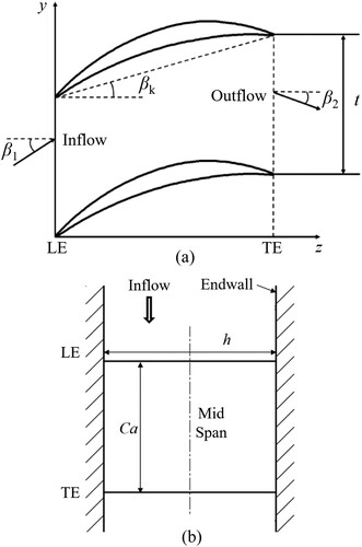
Figure 1. Schematic of baseline cascade: (a) blade-to-blade view; (b) side view. LE = leading edge; TE = trailing edge.

3. CFD methodology, valuations and flow field of baseline cascade

3.1. CFD methodology and validations

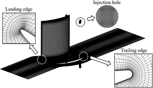
Based on the assumption of periodicity, 3D numerical simulations were performed using the commercial software package NUMECA FINE/Turbo, and the structured mesh of the endwall air injection cascade is shown in Figure 2. The injection hole mesh and the blade passage mesh were joined together with full non-matching connection technology in commercial software package NUMECA IGG. At the inlet boundary of the cascade, the total pressure, total temperature and flow direction are presented. At the outlet boundary, the average static pressure was adopted. For the solid wall boundary, the no-slip wall condition was used. Total pressure, total temperature and flow direction are presented at the inlet boundary of the injection hole; the flow direction was parallel with the axial direction of the injection hole. The inlet boundary of the cascade was located at the 150% axial chord upstream of the leading edge, while the outlet boundary was located at the 200% axial chord downstream of the trailing edge.

Figure 2. Blade surface and endwall mesh of endwall air injection compressor cascade.

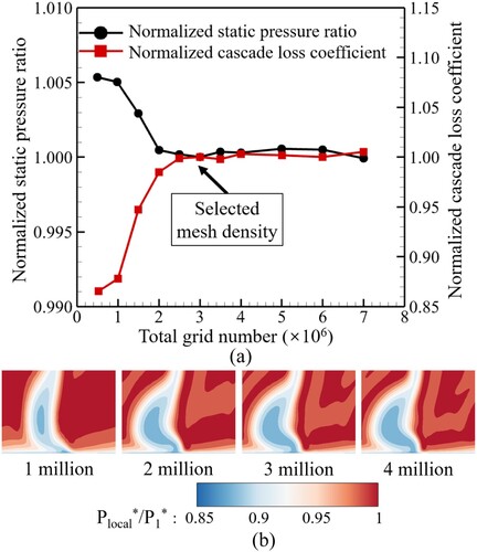
A total grid density of 3.0 million and the Spalart–Allmaras (SA) turbulence model were utilized, as validated in the authors’ previous study on SEAI with the same cascade configuration (Cao et al., 2021). The validation of grid independence is shown in Figure 3. The baseline compressor cascade was simulated with different grid densities ranging from 0.5 to 7 million. In Figure 3(a), the static pressure ratio and the cascade loss coefficient were normalized by the result under the grid density of 3 million. The cascade loss coefficient (ω_ca) was defined as: (1) $\begin{array}{r}{\omega }_{\text{ca}}=\frac{P_1^{\ast }-P_2^{\ast }}{P_1^{\ast }-P_1}\end{array}$(1) where P is static pressure, P* is total pressure, and subscripts 1 and 2 represent the inlet boundary of the cascade and the location at the 150% axial chord section, respectively. It can be seen that the static pressure ratio and the cascade loss coefficient varied obviously when the total grid number was lower than 2.5 million. As the total grid number reached 2.5 million, the static pressure ratio and cascade loss coefficient exhibited slight changes with the increase in total grid number. Figure 3(b) shows the endwall total pressure contour at the 150% axial chord section of the cascade, where the total pressure distribution remained unchanged when the total grid number exceeded 2 million. Therefore, the total grid number of 3 million was selected in this study.

Figure 3. Validation of grid independence: (a) static pressure ratio and cascade loss coefficient; (b) total pressure contour near endwall.

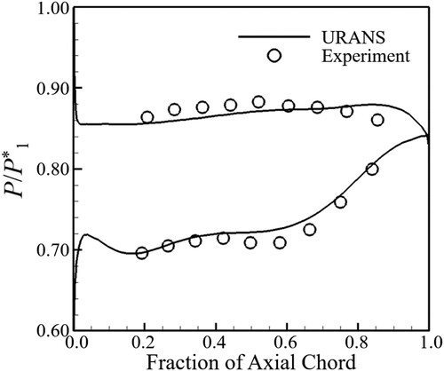
The baseline cascade was experimentally investigated on a high-speed cascade wind tunnel in Northwestern Polytechnical University, PR China (Cao et al., 2014). The measuring section of the cascade wind tunnel is shown in Figure 4. The inlet boundary condition and outlet boundary condition in the numerical simulation were consistent with the results of the experimental measurement. The total pressure of 110,700 Pa, total temperature of 330 K and inflow angle of 40.67° are presented at the inlet boundary, and the static pressure of 95,920 Pa at the outlet boundary. Figure 5 shows the comparison of the time-averaged unsteady numerical results and experimental results of the static pressure distribution of the cascade at mid-span under the design condition, from which it can be seen that the static pressure was well captured.

Figure 4. Measuring section of the cascade wind tunnel (Cao et al., 2014).

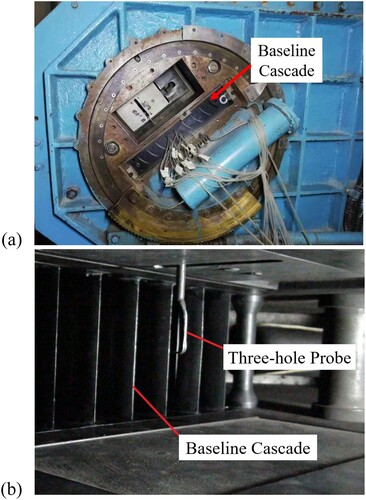
Figure 5. Comparison of numerical results and experimental results of baseline cascade at mid-span. URANS =  Unsteady Reynolds-averaged Navier–Stokes.

Unsteady Reynolds-averaged Navier–Stokes (URANS) equations with an explicit four-stage Runge–Kutta scheme were solved in FINE/TURBO. Several convergence acceleration techniques, such as full multi-grid, dual time stepping and implicit residual smoothing, were employed. The maximum number of iterations within each time-step was set to 20 and the CFL number was 3, which was a parameter controlling the time step. In addition, the steady calculation results were used as the initial solution of the unsteady calculation to accelerate convergence. In total, 20 time steps were calculated in an air injection period.

3.2. Computational flow field analysis of baseline cascade

The flow field of the baseline cascade is shown in Figure 6, including limiting streamlines on solid walls, reverse flow iso-surface, 3D streamlines and axial velocity contour at the exit section of the cascade. From the figure, it can be seen that there was a reversed flow in the suction corner, which led to significant loss of the baseline cascade. Compared with the low-velocity region caused by trailing edge separation, the corner separation was the major source of the loss coefficient in the baseline cascade.

Figure 6. Reverse flow iso-surfaces, axial velocity contour and limiting streamlines of baseline cascade.

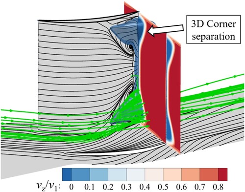
Figure 7 shows the iso-surfaces with the Q-criterion of 0.5 × 10⁶ and contours of the local loss coefficient at axial sections of 145%, 210% and 285% relative axial chord, respectively. The Q-criterion is defined as (Hunt et al., 1988): (2) $\begin{array}{r}Q=\frac{1}{2}\left({||\mathrm{\Omega }||}^2-{||S||}^2\right)\end{array}$(2) The local loss coefficient (ω) is defined as: (3) $\begin{array}{r}\omega =\frac{P_1^{\ast }-P_{\text{local}}^{\ast }}{P_1^{\ast }-P_1}\end{array}$(3) where Ω is the vorticity, S is shear strain rate tensors, and the subscript local represents the local value. All contours on iso-surfaces in this study represent vorticity in the axial direction, where the red color represents the counterclockwise rotating flow and the blue color represents the clockwise rotating flow when viewed from downstream to upstream.

Figure 7. Q-criterion iso-surfaces and contours of local loss coefficient at different axial sections. HP = pressure surface side leg of horseshoe vortex; HS = suction surface side leg of horseshoe vortex; CV = corner vortex; PV = passage vortex; CSV = concentrating shedding vortex.

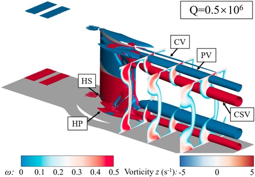
From Figure 7, it can be seen that a series of vortices existed near the endwall of the cascade, and the rotation directions of the same kind of vortices were opposite to each other. Owing to the effect of the cross-passage pressure gradient, the endwall low-momentum fluid rolled up and moved to the suction surface, which led to the formation of a passage vortex. Meanwhile, the pressure surface side leg of the horseshoe vortex moved toward the suction corner of the adjacent blade and finally merged into the passage vortex because of the cross-passage pressure gradient and the same direction of rotation. Compared with the pressure surface side leg, both the spatial scale and stability of the suction surface side leg of the horseshoe vortex were much weaker, and exerted little influence on the flow field. In addition, the low-momentum fluid near the endwall migrated toward the suction corner, resulting in 3D corner separation. As corner separation and trailing edge separation were shed from the cascade, the concentrating shedding vortex formed above the passage vortex. In addition, a typical corner vortex with the same direction of rotation as the passage vortex was found at the endwall corner and trailing edge of the cascade.

4. Schemes of endwall unsteady injection

4.1. Endwall injection hole configuration

Based on the authors’ previous study on single-hole endwall steady injection in the same compressor cascade (Cao et al., 2021), the most effective injection scheme for controlling corner separation was selected for the investigation of unsteady injection in this study. The injection hole, with a diameter of 4 mm, was located at the 74.1% axial chord close to the suction surface. There were two endwall injection holes on both endwalls of the cascade, which were symmetrically placed with 50% blade span section as reference, as shown in Figure 2.

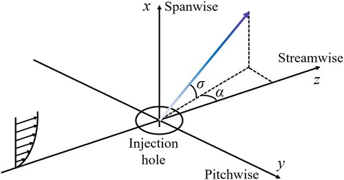
The definition of endwall injection direction is shown in Figure 8, where x is the spanwise direction, y is the pitchwise direction and z is the axial direction. In this study, the angle σ was set to 45° and the angle α was set to 48.8° for the injection hole at the lower endwall; for the other injection hole, the angle σ was set to −45° and the angle α was set to 48.8°, which are optimal steady injection angles of this cascade based on the authors’ previous study (Cao et al., 2021).

Figure 8. Definition of endwall injection direction.

4.2. Pulsed injection computation definition

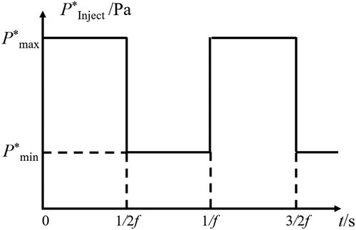
PEAI was carried out under different injection amplitudes and injection frequencies. The pulsed boundary condition of the injection hole is defined as: $P_{\text{inject}}^{\ast }\left(t\right)=\{\begin{array}{l}{P}_{max}^{\ast }\begin{array}{ll}& nT\le t<nT+0.5T\end{array}\\ P_{min}^{\ast }\begin{array}{ll}& nT+0.5T\le t<\left(n+1\right)T\end{array}\end{array}$$\left(n=0,1,2,3\cdots \right)$ (4)where P*_max is the maximum injection total pressure, P*_min is the minimum injection total pressure, t is time, and T is the period of PEAI, which is the reciprocal of injection frequency f. In this study, P*_min is a constant value (93,000 Pa), under which the injection mass flow rate of SEAI can be maintained at 0. The values of P*_max and T depend on the injection amplitude and frequency, respectively. According to Equation (4)(5) $\begin{array}{r}\overline{A}=\frac{P_{max}^{\ast }}{P_1^{\ast }}\end{array}$(5) , the total pressure of the injection hole changed in the form of a square wave with a duty cycle of 0.5, as shown in Figure 9. In this study, the value of the time-step number per air-injection period used in all PEAI cases was 20.

Relevant parameters for PEAI are introduced in the following equations.

Figure 9. Variation of total pressure at the injection hole inlet.

Injection amplitude $\left(\overline{A}\right)$ is defined as: (5) $\begin{array}{r}\overline{A}=\frac{P_{max}^{\ast }}{P_1^{\ast }}\end{array}$(5) Injection frequency is represented by the Strouhal number (St): (6) $\begin{array}{r}St=\frac{fC}{\overline{v_1}}\end{array}$(6) Considering the loss caused by air injection, the mass-weighted approach was adopted in the calculation of the overall loss coefficient (ω_et) (Evans & Hodson, 2011), as shown in Equation (7)(8) $\begin{array}{r}\overline{\omega }=\frac{{\int }_0^T{m}_1\left(t\right)\omega \left(t\right)dt}{{\int }_0^T{m}_1\left(t\right)dt}\end{array}$(8) : (7) $\begin{array}{r}{\omega }_{\text{et}}=\frac{m_1\left(P_1^{\ast }-P_2^{\ast }\right)+m_{\text{jet}}\left(P_{\text{jet}}^{\ast }-P_2^{\ast }\right)}{\left(m_1+m_{\text{jet}}\right)\left(P_1^{\ast }-P_1\right)}\end{array}$(7) The time-averaged loss coefficient is defined as: (8) $\begin{array}{r}\overline{\omega }=\frac{{\int }_0^T{m}_1\left(t\right)\omega \left(t\right)dt}{{\int }_0^T{m}_1\left(t\right)dt}\end{array}$(8) The static pressure coefficient (Cp) is defined as: (9) $\begin{array}{r}Cp=\frac{P_{\text{local}}-P_1}{P_1^{\ast }-P_1}\end{array}$(9) where P is static pressure, P* is total pressure, m is mass flow rate, C is the chord length of the cascade, v is the velocity, and subscripts 1, 2, local and jet represent the inlet boundary of the cascade, 150% axial chord section, local value and injection inlet boundary, respectively.

Considering the mixing loss between the mainstream and the injection flow, the accurate entropy generation of the PEAI cascade during the mixing process (Young & Horlock, 2006) was calculated. For the PEAI cascade in this study, the entropy generation (Δs) is defined as: (10) $\begin{array}{rl}\Delta s& =\left(\frac{m_1}{m_2}\right)\left[C_p\ln \left(T_2^{\ast }-T_1^{\ast }\right)-R\ln \left(\frac{m_1{P}_2^{\ast }}{m_2{P}_1^{\ast }}\right)\right]\\ & +\left(\frac{m_{\text{jet}}}{m_2}\right)\left[C_p\ln \left(T_2^{\ast }-T_{\text{jet}}^{\ast }\right)-R\ln \left(\frac{m_{\text{jet}}{P}_2^{\ast }}{2m_2{P}_{\text{jet}}^{\ast }}\right)\right]\end{array}$(10) where C_p is specific heat capacity, R is the specific gas constant, and T* is total temperature. Assuming that the injection flow and the mainstream were completely mixed, the entropy generation during the mixing process accounted for 13.3% of the total entropy generation, which was a small proportion. The mixing loss is not the main concern of this study, but, rather, the loss caused by flow separation and vortical structures. In addition, the mixing loss can be reflected in the decrease in total pressure. Therefore, the definition of the loss coefficient can be used to evaluate the loss generation in the whole cascade passage in a comprehensive way.

5. Results and discussion

5.1. Influence of pulsed endwall air injection on time-averaged performance and flow field of compressor cascade

In the existing literature (Gmelin et al., 2010, 2012; Meng et al., 2018; Zheng et al., 2005, 2006, 2011), the St value of pulsed air injection ranged from 0 to 2. In the authors’ previous SEAI study on an identical cascade, the injection amplitude was 1.22, under which the endwall loss coefficient (ω_ew) was reduced significantly and the corner separation was controlled effectively (Cao et al., 2021). In this study, the injection frequency of PEAI was set from 0 to 4500 Hz (St ranging from 0 to 1.463) and the injection amplitude of PEAI ranged from 0.87 to 1.40.

Figure 10 shows the time-averaged cascade loss coefficient (ω_ca) and overall loss coefficient (ω_et) of PEAI cases under four injection amplitudes (0.87, 1.00, 1.22 and 1.40) and different injection frequencies. Except for the injection amplitude of 0.87, both ω_ca and ω_et of PEAI cases showed a tendency toward first decreasing and then increasing with St, so the selected range of injection frequencies was appropriate.

Figure 10. Cascade loss coefficient and overall loss coefficient of different pulsed endwall air injection (PEAI) cases: (a) time-averaged cascade loss coefficient; (b) time-averaged overall loss coefficient.

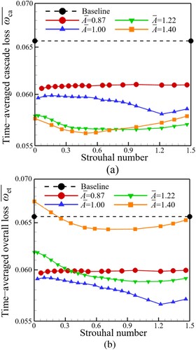
Since the injection strength of PEAI cases under the injection amplitude of 0.87 was too weak, the variation of St had little effect on the loss coefficients. In Figure 10(a), the PEAI cases under the injection amplitude of 1.22 and 1.40 provided sufficient high-momentum injection fluid, which improved the flow field in the corner, and the cascade loss coefficients reached a low level. Considering the loss brought about by air injection, the variation of the overall loss coefficient in Figure 10(b) indicated that the lowest loss was achieved under the injection amplitude of 1.00, and the loss coefficient of the scheme with the injection amplitude of 1.40 reached a similar magnitude to the baseline cascade. Therefore, the range of injection amplitude was set from 0.87 to 1.40.

The numerical results showed that the corner separation could not be effectively controlled by SEAI and PEAI when the injection amplitude was lower than 1.22 (in Section 5.2). Therefore, the cases in which the injection amplitude was set to 1.22 and 1.40 were analyzed in the following.

In Figure 11, four typical PEAI cases with different injection frequencies (St = 0.002, 0.488, 0.975 and 1.463) and SEAI cases are compared. It is shown that the loss coefficients were reduced significantly after applying SEAI and PEAI; the maximum reduction of the cascade loss coefficient and overall loss coefficient loss was 14.5% and 10.5%, respectively. In Figure 11(a), the time-averaged cascade loss coefficient under different St values was approximately the same as that of SEAI, and the minimum cascade loss coefficients with injection amplitudes of 1.22 and 1.40 were lower than those of the SEAI results under the same injection amplitudes. The minimum time-averaged cascade loss coefficient was 14.5% lower than that of the baseline cascade. These results indicate that PEAI can achieve approximately the same control effect on the corner separation as that of SEAI, even under lower injection mass flow. The overall loss coefficients of the SEAI and time-averaged PEAI cases are shown in Figure 11(b). It is worth noting that the overall loss coefficient of the SEAI cases was higher than that of the baseline cascade, which means that the SEAI brought additional injection loss while suppressing flow separations. In contrast to Figure 11(a), overall loss coefficients of both injection amplitudes reached the lowest value when St was 0.975. Compared with the baseline cascade, the overall loss coefficients of the PEAI cases with injection amplitudes of 1.22 and 1.40 were reduced by 10.5% and 2.1%, respectively. This indicates that PEAI cases exhibited lower overall loss coefficients compared with SEAI cases.

Figure 11. Cascade loss coefficient and overall loss coefficient of different cases: (a) time-averaged cascade loss coefficient; (b) time-averaged overall loss coefficient.

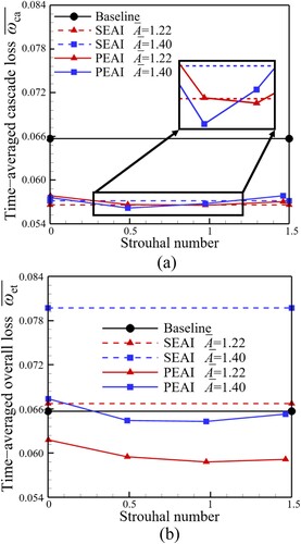
From the above analysis, although the PEAI case with an injection amplitude of 1.40 achieved the lowest cascade loss coefficient (St = 0.488 in Figure 11a), the high injection amplitude led to significant injection loss, which made the overall loss coefficient of PEAI nearly the same as that of the baseline cascade. By contrast, the PEAI case (St = 0.975, $\overline{A}$ = 1.22) significantly reduced the overall loss coefficient. Therefore, the PEAI case (St = 0.975, $\overline{A}$ = 1.22) was regarded as the optimal PEAI case in this study. The analysis in the following paragraphs will be carried out based on this case.

Figure 12 shows the comparison of the endwall loss coefficients of the baseline cascade, the optimal PEAI case and the SEAI case under $\overline{A}$ = 1.22. The endwall loss coefficient (ω_ew) was calculated with the aerodynamic parameter of 20% cascade mass flow near the endwall (Taylor & Miller, 2017). It can be seen that the SEAI case significantly reduced endwall loss compared with the baseline cascade, with a rate of reduction of 39.4%, which indicates that the corner separation was suppressed effectively with SEAI (Cao et al., 2021). Compared with the baseline cascade, the endwall loss coefficient of the optimal PEAI case was reduced by 28.7%, indicating that PEAI had a less significant control effect on corner separation than SEAI. Although SEAI exhibited a better control effect near the endwall, it brought more loss at mid-span than PEAI, which resulted in a higher overall loss coefficient.

Figure 12. Endwall loss coefficient of different cascades. SEAI = steady endwall air injection; PEAI = pulsed endwall air injection.

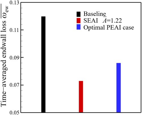
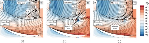
Figure 13 shows the distribution of the static pressure coefficient (Cp) and limiting streamlines on the suction surface and endwall of the baseline cascade, SEAI cascade ($\overline{A}$ = 1.22) and optimal PEAI cascade. It can be seen that there is a separation line consisting of the trailing edge separation line and the corner separation line along the whole blade span. Compared with the baseline cascade, both SEAI and PEAI cascades exhibited increased Cp on the suction surface and endwall near the trailing edge. On the one hand, the injection fluid brought enough streamwise momentum to the separation fluid, which promoted the reattachment of near-wall flow. On the other hand, the spanwise momentum caused the fluid in the suction corner to migrate toward the mid-span, and the blockage in the suction corner was reduced. Therefore, SEAI significantly suppressed the corner separation. However, as the low-momentum fluid migrated toward and accumulated at the mid-span, the trailing edge separation was increased under a higher streamwise pressure gradient. Compared with SEAI, PEAI exhibited a weaker control effect on corner separation, and thus reduced the mid-span flow field less significantly.

Figure 13. Time-averaged Cp contour and limiting streamlines on the suction surface and endwall of cascades: (a) baseline cascade; (b) steady endwall air injection (SEAI) cascade ($\overline{A}$ = 1.22); (c) optimal pulsed endwall air injection (PEAI) cascade (St = 0.975, $\overline{A}$ = 1.22). LE = leading edge; TE = trailing edge; CSL = corner separation line; TSL = trailing separation line.

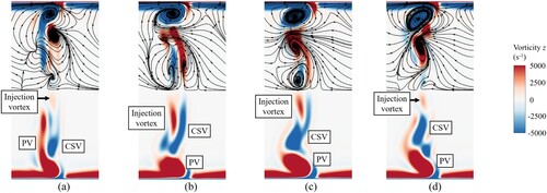
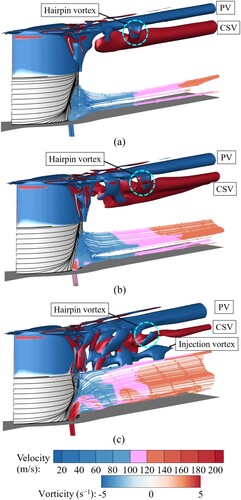
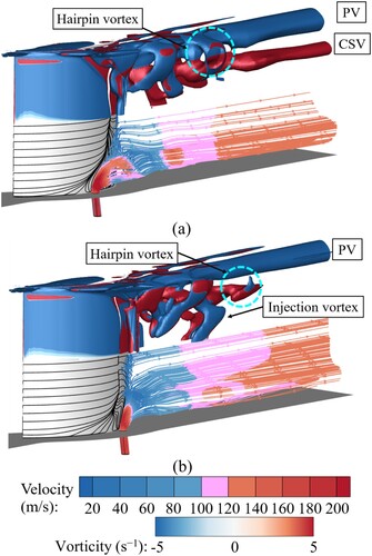
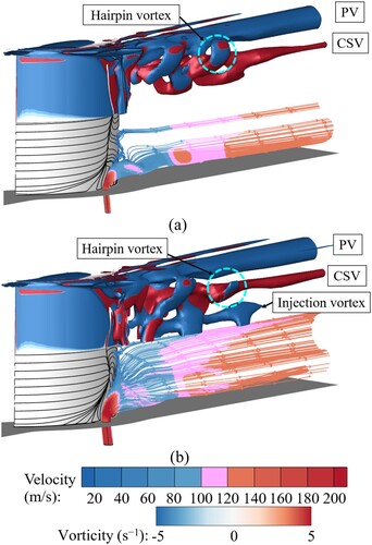
In total, 20 time steps were calculated in an air injection period. Figure 14 shows the transient flow fields at four equally spaced times steps during one injection period of the optimal PEAI cascade. Compared with the baseline cascade in Figure 7, the spatial scale of the concentrating shedding vortex was obviously reduced after applying the optimal PEAI. After mixing the high-velocity injection flow with low-momentum fluid in the suction corner, the mixed flow was divided into three branches, distributed in the ranges 0–20%, 20–40% and 40–50%, respectively. The first two branches eventually flowed into the passage vortex and concentrating shedding vortex, respectively. After PEAI, the high-velocity injection fluid periodically forced a portion of the passage vortex and concentrating shedding vortex to migrate toward the injection direction and squeeze each other, which led to the formation of a hairpin vortex distributed at equal intervals. The vortex has previously been observed in a study on film cooling (Zhong et al., 2016), but the authors have not found it in a compressor cascade with air injection. Because the directions of rotation of the passage vortex and the concentrating vortex were opposite to each other, the interaction between them (the hairpin vortex with a disordered axial vorticity) reduced their intensity, especially for the concentrating shedding vortex. With the extension of time, the hairpin vortex moved downstream while a new hairpin vortex formed from the trailing edge near the suction corner.

Figure 14. Transient vortex structures and distributions of injection flow at different times [optimal pulsed endwall air injection (PEAI) cascade, Q = 5 × 10⁵ s⁻²]: (a) t = 0T/20; (b) t = 5T/20; (c) t = 10T/20; (d) t = 15T/20. PV = passage vortex; CSV = concentrating shedding vortex.

Apart from the hairpin vortex, a new vortex named the injection vortex appeared at the mid-span of the cascade passage. The mechanism of formation of the injection vortex was more complex. Figure 15 shows the transient flow field of the optimal PEAI cascade at 10T/20, including the contour of axial vorticity at the 150% axial chord section and streamlines across the injection vortex region. It can be seen that the injection vortex consisted of three parts of fluid: (1) the low-momentum fluid on the suction surface; (2) the low-momentum fluid near the endwall; and (3) the injection fluid from the injection holes. After PEAI, these three parts of the fluid migrated toward the mid-span and shed from the trailing edge. In addition, the passage vortex and concentrating shedding vortex expanded to the mid-span. Regarding the effect of the expanded concentrating shedding vortex, the fluid near the mid-span periodically rolled up the injection vortex, with the opposite direction of rotation to the concentrating shedding vortex.

Figure 15. Transient distribution of streamlines forming the injection vortex [optimal pulsed endwall air injection (PEAI) cascade, t = 10T/20]. PV = passage vortex; CSV = concentrating shedding vortex.

Figure 16 shows the transient axial vorticity contour and limiting streamlines at the 150% axial chord section of the optimal PEAI cascade during an injection period. The flow field at different time steps showed that the intensity of the injection vortex was mainly affected by the concentrating shedding vortex. As the hairpin vortex flowed through the axial section with time, high-vorticity regions of the passage vortex and concentrating shedding vortex exhibited obviously spanwise extension. When the concentrating shedding vortex expanded to the mid-span, the accumulated low-momentum fluid rolled up the obvious injection vortex, as shown in Figure 16(b) and (c). Because the injection vortex was too weak to be maintained, it dissipated rapidly as it flowed downstream. In addition, Figure 16(d) shows that a weak vortex rolled up between the passage vortex and concentrating shedding vortex because of the spanwise extended passage vortex.

Figure 16. Transient axial vorticity contour and limiting streamlines of the optimal cascade at 150% axial chord section: (a) t = 0T/20; (b) t = 5T/20; (c) t = 10T/20; (d) t = 15T/20. PV = passage vortex; CSV = concentrating shedding vortex.

5.2. Effect of injection amplitude on flow field in PEAI cascade

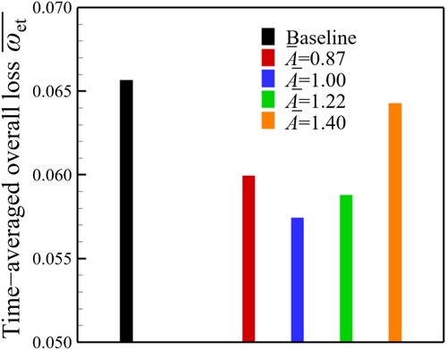
When the St value was 0.975, the cascade loss and overall loss of most PEAI cases were relatively low, and the St value of the optimal PEAI case was also 0.975. Therefore, the St value of 0.975 was selected to investigate the effect of injection amplitude ($\overline{A}$) on the PEAI cascade.

Figure 17 shows the time-averaged overall loss coefficient under different injection amplitudes with an St value of 0.975. It is shown that the time-averaged overall loss coefficient of the cascade was reduced significantly after applying PEAI. As the injection amplitude increased, the time-averaged overall loss coefficient showed a tendency to first decrease and then increase. The optimal injection amplitude reduced the time-averaged overall loss coefficient by 12.5% at most, with the injection amplitude of 1.0. The increased overall loss was a result of the higher injection mass flow rate.

Figure 17. Variation of time-averaged overall loss coefficient under different injection amplitudes (St = 0.975).

The time-averaged flow fields of the endwall and suction surface of the compressor cascade under different injection amplitudes are presented in Figure 18. Compared with the baseline cascade in Figure 13(a), the area of the high static pressure region on both the endwall and suction surface expanded significantly, which indicates that the diffusion ability of the cascade was improved after applying PEAI. Regarding the effect of the injection fluid, the endwall low-momentum fluid migrated toward the mid-span. The higher the injection amplitude provided by PEAI, the more energy was obtained by the endwall low-momentum fluid. Therefore, with the increase in the injection amplitude, the 3D corner separation region was suppressed, and the flow separation near the mid-span increased owing to the accumulation of the low-momentum fluid. When the injection amplitude was 1.40, there was no reversed flow in the suction corner, indicating that the 3D corner separation was removed completely. As the injection amplitude was lower than 1.0, the spanwise region of the corner separation line increased with the injection amplitude. However, as this increase in the spanwise region of corner separation line was caused by the spanwise migration of the corner fluid, it does not indicate that the corner separation was increased. As more low-momentum fluid migrated toward the mid-span, the trailing edge separation was increased, as shown in Figure 18(c).

Figure 18. Cp contours and limiting streamlines on the suction surface and endwall (St = 0.975): (a) $\overline{A}$ = 0.87; (b) $\overline{A}$ = 1.00; (c) $\overline{A}$ = 1.40. LE = leading edge; TE = trailing edge; CSL = corner separation line; TSL = trailing separation line.

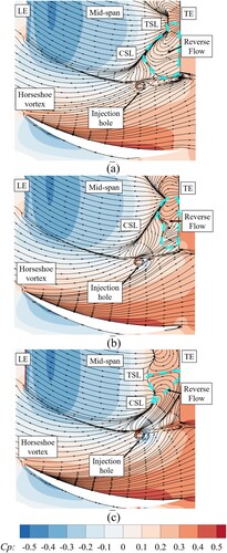
Figure 19 shows the spanwise distribution of the time-averaged local loss coefficient of PEAI cases with an St value of 0.975. Compared with the baseline cascade, the loss of all PEAI cases was reduced in the region from 0% to 26% blade span. For PEAI cases with injection amplitudes lower than 1.00, the loss near mid-span was the same as that of the baseline cascade, and the loss was slightly increased in the range between 30% and 40% spanwise owing to the spanwise migration of low-momentum fluid. Under injection amplitudes higher than 1.00, low-momentum fluid migrated to the mid-span, so the cascade loss between 25% and 50% blade span increased significantly compared with that of the baseline cascade. Meanwhile, since the corner separation was effectively controlled, the loss near the endwall of PEAI cases with high injection amplitude was reduced significantly.

Figure 19. Time-averaged local loss coefficient distribution along spanwise at 150% relative axial chord (St = 0.975).

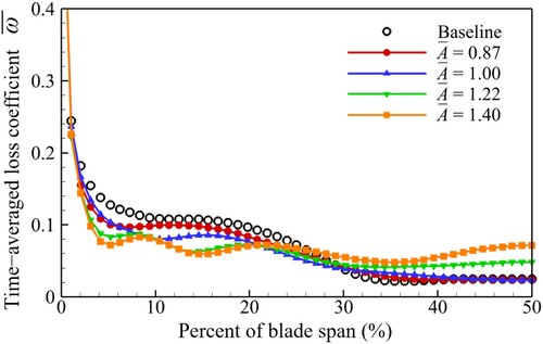
Figure 20 shows the comparison of the static pressure coefficient distribution at 5% and 50% blade span under different injection amplitudes. At 5% blade span, PEAI cases under lower injection amplitudes (0.87 and 1.00) made the location of corner separation move downstream, whereas the corner separation was effectively controlled under higher injection amplitudes. As the injection amplitude increased, the blade loading from the 0.3 axial chord to the trailing edge and the diffusion capability were improved gradually. At the mid-span, too much low-momentum fluid migrated toward the mid-span, so the mid-span flow field deteriorated with the increase in injection amplitude, which is consistent with the results in Figures 18 and 13(c).

Figure 20. Cp distribution of cascade under different injection amplitudes at 5% and 50% spanwise: (a) 5% blade span; (b) 50% blade span.

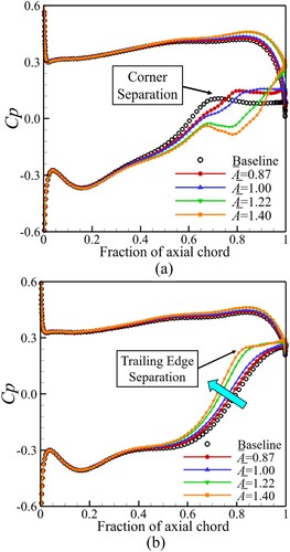
Figure 21 shows the time-averaged 3D vortex structure and local loss coefficient contours at different axial sections under different injection amplitudes. Under low injection amplitudes, as shown in Figure 21(a) and (b), low-momentum fluid migrated toward 30–40% blade span, causing expansion of the concentrating shedding vortex and contraction of the passage vortex compared with the baseline cascade. Because the injection amplitude was insufficient, after time averaging, there was no injection vortex at the mid-span. Under high injection amplitudes, as shown in Figure 21(c) and (d), since the low-momentum fluid was blown toward the mid-span and mixed with the bulk stream, the concentrating shedding vortex decreased rapidly while the mid-span loss increased significantly. Meanwhile, because of the enhancement of the cross-passage pressure gradient at the endwall (as shown in Figure 20), more endwall low-momentum fluid migrated to the suction corner, leading to an increase in the passage vortex. Under an injection amplitude of 1.40, two stable injection vortices appeared at the mid-span after time averaging. The direction of rotation of the injection vortex was opposite to that of the adjacent concentrating shedding vortex.

Figure 21. Time-averaged Q-criterion iso-surfaces and contours of local loss coefficient of pulsed endwall air injection (PEAI) cases (Q = 5 × 10⁵ s⁻²): (a) $\overline{A}$ = 0.87; (b) $\overline{A}$ = 1.00; (c) $\overline{A}$ = 1.22; (d) $\overline{A}$ = 1.40. HP = pressure surface side leg of horseshoe vortex; HS = suction surface side leg of horseshoe vortex; CV = corner vortex; PV = passage vortex; CSV = concentrating shedding vortex.

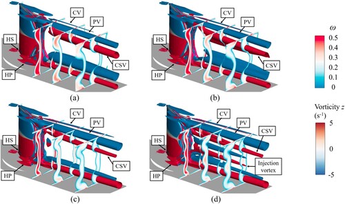
Figure 22 shows the comparison of time-averaged secondary flows and vorticity magnitude contours at the 50% axial chord downstream of the blade trailing edge of the baseline cascade and PEAI cascades under different injection amplitudes. For the baseline cascade, the passage vortex and concentrating shedding vortex occurred. Compared with the baseline cascade, under an injection amplitude of 0.87, the distribution area of high vorticity magnitude was reduced near the endwall, and the concentrating shedding vortex increased because of the migration of low-momentum fluid. As the injection amplitude increased, the pitchwise area of the high vorticity region decreased near the endwall but increased near the mid-span, which was due to the migration of low-momentum fluid. Meanwhile, the suppression of corner separation weakened the concentrating shedding vortex, which relieved the blockage caused by the concentrating shedding vortex and produced more space for the development of the passage vortex. As the injection amplitude reached 1.40, the migration of low-momentum fluid eventually led to the occurrence of an injection vortex, as shown in Figure 22(d).

Figure 22. Time-averaged secondary flow and vorticity contours at 150% axial chord: (a) baseline cascade; (b) $\overline{A}$ = 0.87; (c) $\overline{A}$ = 1.22; (d) $\overline{A}$ = 1.40. CSV = concentrating shedding vortex; PV = passage vortex.

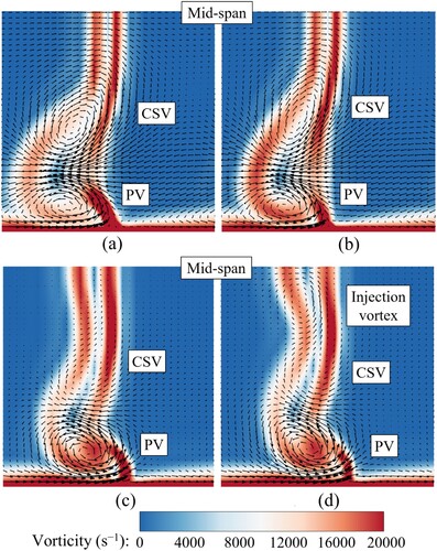
Figure 23 shows the variations in both the cascade loss coefficient (ω_ca) and overall loss coefficient (ω_et) during an entire PEAI period. As shown in Figure 23(a) (the injection loss was not taken into account), it can be seen that the loss in all PEAI cases was reduced at all time steps. However, the variation trends of cascade loss were not consistent with the authors’ expectation, i.e. lower loss in the first half injection period and higher loss in the last half injection period. Under a low injection amplitude of 0.87, the loss coefficient was almost constant, which was due to the damping in the injection hole. As the injection amplitude increased, the cascade loss coefficient increased in the first few time steps and then decreased significantly to the minimum value. The maximum reduction of transient loss was obtained when the injection amplitude was 1.40. The time step number of extreme points decreased with the improvement of the injection amplitude.

Figure 23. Variation of loss coefficients with time step under different injection amplitudes: (a) cascade loss coefficient; (b) overall loss coefficient.

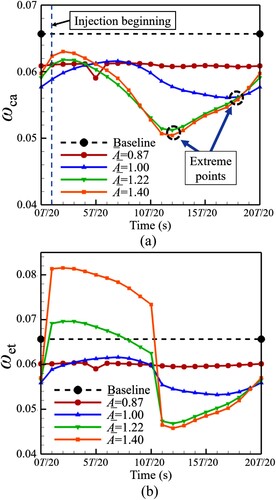
The reason for the characteristics of the cascade loss coefficient in Figure 23(a) was that a higher injection amplitude is related to a higher injection velocity, and therefore the injection fluid will spend less time flowing across the injection hole. Therefore, a smaller time interval existed before the injection began to have an influence on the flow field, and the minimal loss coefficient was found during the final 10 time steps under high injection amplitudes. This detailed flow characteristic will be explained in detail in Section 5.3. In Figure 23(b), the overall loss coefficient was improved in the first 10 time steps, and it increased with injection amplitude. For the last 10 time steps, the overall loss coefficient decreased significantly; as the injection amplitude increased, the overall loss coefficient decreased.

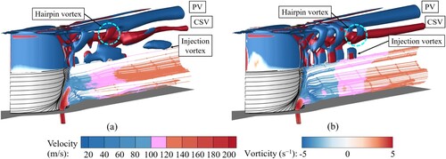
The transient vortex structure and distribution of injection flow with the St value of 0.975 at 10T/20 under different injection amplitudes are shown in Figure 24; the transient flow field of injection amplitude $\overline{A}$ = 1.22 was shown earlier, in Figure 14(c). Under low injection amplitude ($\overline{A}$ = 0.87 and 1.00), the spatial scale of the hairpin vortex was tiny and the injection fluid did not directly affect the flow field at the mid-span. Owing to the migration of low-momentum fluid, the concentrating shedding vortex increased. Under high injection amplitude ($\overline{A}$ = 1.22 and 1.40), as shown in Figures 14(c) and 24(c), the spatial scale of the hairpin vortex increased; at the mid-span, there were obvious injection vortices, which were caused by the mid-span low-momentum fluid and the spanwise expanded concentrating vortex caused by PEAI. However, these injection vortices still failed to form a stable vortex in the mid-span when the injection amplitude was 1.40.

Figure 24. Transient vortex structures and distributions of injection flow (t = 10T/20, Q = 5 × 10⁵ s⁻²): (a) $\overline{A}$ = 0.87; (b) $\overline{A}$ = 1.00; (c) $\overline{A}$ = 1.40. PV = passage vortex; CSV = concentrating shedding vortex.

In summary, under the St value of 0.975, the PEAI cases with higher injection amplitude exhibited a better flow control effect in the suction corner, thus effectively suppressing the corner separation. However, owing to the spanwise migration of low-momentum fluid under injection, the flow field near the mid-span deteriorated. The periodical PEAI led to a series of hairpin vortices, distributed at equal intervals.

5.3. Effect of injection frequency on flow field in PEAI cascade

Under an injection amplitude of $\overline{A}$ =  1.22, the injection frequency effect was studied. Figure 25 shows the variation of the overall loss coefficient under different injection frequencies (St = 0.002, 0.488, 0.975 and 1.463). The results showed that as the injection frequency increased, the overall loss coefficient showed a tendency to first decrease and then increase. The time-averaged cascade loss coefficient of the optimal PEAI case (St = 0.975) reached a minimum value of 0.0588, which was lower than that of the SEAI case under the same injection amplitude.

Figure 25. Variation of time-averaged overall loss coefficient under different injection frequencies ($\overline{A}$ = 1.22).

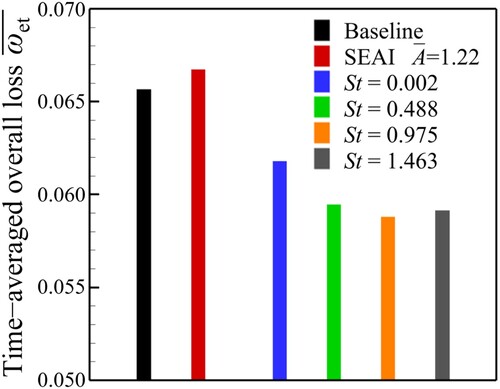
Figure 26 shows the distribution of the time-averaged local loss coefficient along the spanwise under different injection frequencies. Both SEAI and PEAI suppressed endwall loss but intensified mid-span loss. It is worth noting that SEAI had a larger influence on loss than PEAI along the whole blade span. As St increased, the loss of the whole blade span gradually decreased and then tended to become stable. The Cp distribution shown in Figure 27 indicates that higher St values correspond to higher endwall loading and more severe trailing edge separation at the mid-span.

Figure 26. Time-averaged local loss coefficient distribution along spanwise at 150% relative axial chord ($\overline{A}$ = 1.22).

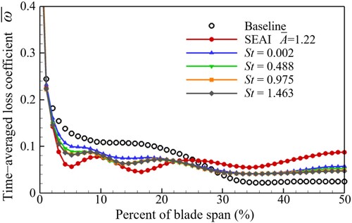
Figure 27. Cp distribution of cascade under different injection amplitudes at 5% and 50% spanwise: (a) 5% blade span; (b) 50% blade span.

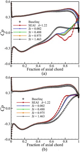
Figure 28 shows the variations of the cascade loss coefficient (ω_ca) and overall loss coefficient (ω_et). In Figure 28(a), the PEAI reduced cascade loss effectively at every time step. Under an St of 0.002, the variation curve of loss showed a convex shape in the first 10 time steps and the final 10 time steps, which was inconsistent with expectations, i.e. the cascade loss stayed at a low level in the first 10 time steps and maintained a high level in the final 10 time steps. The reason for these two convex shapes was that the PEAI had enough time to change the flow field at low injection frequency, so that the flow fields before and after 10T/20 and 20T/20 were completely different. The sudden change in the flow field led to a strong effect of mixing and viscous dissipation in the suction corner, and therefore the cascade loss coefficient increased within a few time steps. In Figure 28(b), the overall loss coefficient of all PEAI cases increased in the first 10 time steps and decreased in the final 10 time steps. In addition, under high injection frequencies (St = 0.488, 0.975 and 1.463), the maximum reduction of transient loss decreased with the increase in St.

Figure 28. Variation of loss coefficients with time step under different injection frequencies: (a) cascade loss coefficient; (b) overall loss coefficient.

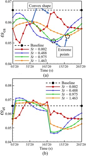
The variation of the cascade loss coefficient under high St was distinctly different from that under low St. The time step number of extreme points increased with the St, and the relevant flow mechanism is explained in Figures 29 and 30.

Figure 29. Transient velocity distribution of a section of endwall injection hole (St = 0.975).

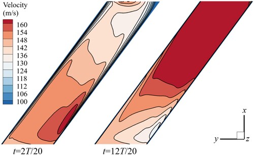
Figure 30. Variation of injection velocity with time step under different injection frequencies. PV = passage vortex; CSV = concentrating shedding vortex.

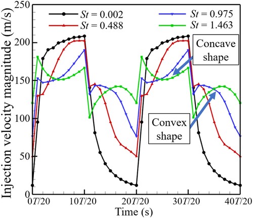
Table 1. Main geometric and aerodynamic parameters of the cascade.

Parameter	Notation	Data
Chord (mm)	C	65
Inflow angle (°)	β1	40.67
Outflow angle (°)	β2	−13.21
Stagger angle (°)	βk	15.4
Aspect ratio	h/C	1.54
Solidity	τ	1.66
Inflow Mach number	Ma1	0.6
Reynolds number	Re	9.01 × 10^5
2D diffusion factor	D	0.42

Unlike the PEAI case under low injection frequency (St = 0.002), for PEAI cases with a high injection frequency, the magnitude of the temporal scale of a single time step reached the same level as when the injection fluid flowed across the injection hole. In the case with St = 0.975, the time required for the injection fluid to flow across the hole was approximately 7.5 × 10⁻⁵s; the actual time of each time step was 1.67 × 10⁻⁵s, so the injection flow required about 4.5 time steps to flow across the hole. When there was a sudden total pressure change at the inlet of the injection holes at the end of every 10 time steps, the fluid that had not flowed out of the hole would interact with the new injection flow until the previous fluid in injection holes had completely drained, which indicates that there was an inertia effect for the flow in the injection hole, as shown in Figure 29.

Figure 30 shows the injection velocity magnitude at each time step for two continuous periods under different injection frequencies. Compared with the transient total pressure distribution at the injection hole, the transient variation of injection velocity did not exhibit a square wave in shape. As the St value increased, the amplitude of the injection velocity reduced significantly. Under St of 0.975 and 1.463, the velocity variation curve showed a concave shape in the first 10 time steps and a convex shape in the second 10 time steps, which indicates that a stronger inertia effect occurred under higher St. Above all, the inertia was a special unsteady effect in the PEAI cascade, which increased with the increase in frequency.

To investigate the vortex structure under different injection frequencies, and especially the influence of the initial injection phase on the baseline flow field, the flow field under an injection frequency of 0.002 was selected because it had the weakest unsteady effect of inertia.

Figure 31 shows the transient vortex structures and distributions of injection flow at four equally spaced time steps during one injection period (St = 0.002). At the time of 0T/20 (the time step just before the beginning of air injection), there were few low-velocity injection flows distributing in the region between 0% and 30% blade span. The injection flow was divided into two branches, which mixed with the low-momentum fluid in the suction corner and then developed into the passage vortex and concentrating shedding vortex, respectively. At the time of 5T/20, the high-velocity injection flow caused much of the low-momentum fluid to migrate to the mid-span, and the injection flow was divided into three branches. On the one hand, the concentrating shedding vortex was suppressed by the injection flow. On the other hand, the low-momentum fluid accumulating near the mid-span rolled up a new injection vortex due to the effect of the concentrating shedding vortex as the injection remained stable at the time of 10T/20. Finally, the injection vortex disappeared with the decrease in low-momentum fluid near the mid-span at the time of 15T/20. Compared with the low-frequency case (St = 0.002, Figure 31), the variation of flow fields of the high-frequency case (St = 0.975, Figure 14) at different time steps was more moderate because of the strong unsteady effect of inertia.

Figure 31. Transient vortex structures and distributions of injection flow at different time steps (St = 0.002, $\overline{A}$ = 1.22, Q = 5 × 10⁵ s⁻²): (a) t = 0T/20; (b) t = 5T/20; (c) t = 10T/20; (d) t = 15T/20. PV = passage vortex; CSV = concentrating shedding vortex.

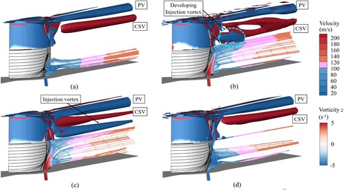
Figure 32 shows the transient flow field of different injection frequencies (St = 0.488, 1.463) at the time of 10T/20. The flow fields of different injection frequency cases at St = 0.002 and 0.975 have been shown previously in Figures 31(c) and 14(c). The passage vortices of all different injection frequency cases were approximately the same. As the injection frequency increased, the intensity of the concentrating shedding vortex increased. However, owing to the interaction of PEAI, the shape of the concentrating shedding vortex was no longer a regular streamwise vortex, but, rather, a distorted vortex. As the injection frequency exceeded 0.488, a hairpin vortex appeared near the endwall. It can be seen from Figure 32 that the interval between adjacent hairpin vortices decreased as the injection frequency increased.

Figure 32. Transient vortex structures and distributions of injection flow (t = 10T/20, Q = 5 × 10⁵ s⁻²): (a) St = 0.488; (b) St = 1.463. PV = passage vortex; CSV = concentrating shedding vortex.

In summary, there existed an optimal injection frequency under which the cascade exhibited the best performance. The inertia derived from the interaction of injection air with different velocities intensified with the increase in the injection frequency. Under a low injection frequency, the length of a single time step was long enough to allow the injection flow to flow through the injection hole, so the difference among flow fields became obvious over time. Under high St, the variation of flow fields with time was moderate because of the strong effect of inertia.

5.4. Effect of injection hole location on PEAI

To further investigate the effect of injection locations on the flow field of the PEAI cascade, two new single-hole PEAI schemes were designed, which are named the Lead-PEAI case and the Trail-PEAI case. The initial injection location investigated in the Section 5.1 named the Mid-PEAI case in this subsection. The new injection holes were located at the 62.9% and 85.3% axial chords of the cascade, as shown in Figure 33. Based on the previous subsections, the Lead-PEAI case and Trail-PEAI case were numerically simulated under the optimal injection parameters, i.e. with an St value of 0.975 and injection amplitude of 1.22.

Figure 33. Pulsed endwall air injection (PEAI) cases at different injection locations.

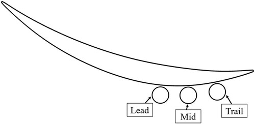
Figure 34 shows the time-averaged cascade loss coefficient, overall loss coefficient and endwall loss coefficient of SEAI cases and PEAI cases at different injection locations. As the injection location moved to the trailing edge, the time-averaged cascade loss coefficient and overall loss coefficient of both SEAI and PEAI cases decreased. As shown in Figure 34(a), the Mid-PEAI case and Trail-PEAI case achieved the same control effect as that of the SEAI cases, and the Trail-PEAI case exhibited the lowest cascade loss coefficient. After considering the injection loss (Figure 34b), the injection loss of the PEAI cases was much lower than that of the SEAI cases, indicating the significant advantage of PEAI in mass flow consumption. From Figure 34(c), the variation trends of the time-averaged endwall loss of SEAI cases and PEAI cases were opposite to each other, and the endwall loss of the PEAI case was higher than that of the SEAI case at the same injection location.

Figure 34. Variation of time-averaged cascade loss coefficient and endwall loss coefficient: (a) time-averaged cascade loss coefficient; (b) time-averaged overall loss coefficient; (c) time-averaged endwall loss coefficient. SEAI = steady endwall air injection; PEAI = pulsed endwall air injection.

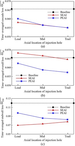
Figure 35 shows the time-averaged flow field of PEAI cases at different injection locations. Compared with Figure 13(c), there was only a corner separation line on the suction surface of the Lead-PEAI case and the separation region near the mid-span decreased significantly. However, near the endwall, the movement of the injection hole caused the migration of the corner separation line toward the leading edge, which led to an increase in the endwall loss. For the Trail-PEAI case, the corner separation line migrated toward the trailing edge while the effect region of trailing edge separation increased. The Trail-PEAI case effectively controlled the corner separation and improved the diffusion ability of the cascade. The control mechanism was the concentrating shedding vortex in the Trail-PEAI case, which was completely controlled by air injection, as shown in Figure 36(b). The low-momentum fluid gathered near 20% blade span was directly blown downstream by PEAI and the concentrating shedding vortex dissipated in a short axial distance.

Figure 35. Distribution of Cp and limiting streamlines of pulsed endwall air injection (PEAI) cases at different injection locations (St = 0.975, $\overline{A}$ = 1.22): (a) Lead-PEAI case; (b) Trail-PEAI case. LE = leading edge; TE = trailing edge; CSL = corner separation line; TSL = trailing separation line.

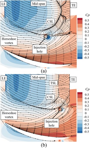
Figure 36. Time-averaged Q-criterion iso-surfaces and contours of local loss coefficient at different injection locations (St = 0.975, $\overline{A}$ = 1.22, Q = 5 × 10⁵ s⁻²): (a) Lead-PEAI case; (b) Trail-PEAI case. HP = pressure surface side leg of horseshoe vortex; HS = suction surface side leg of horseshoe vortex; CV = corner vortex; PV = passage vortex; CSV = concentrating shedding vortex.

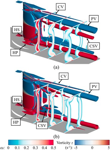
Figure 37 shows the secondary flows and vorticity contours at the 50% axial chord downstream of the cascade at different PEAI locations. Compared with the baseline cascade in Figure 22(a), the strength of secondary flows was reduced significantly after PEAI. Compared with the Mid-PEAI case, since the Lead-PEAI case had a larger region of effect in the suction corner, both the passage vortex and concentrating shedding vortex migrated toward the mid-span. For the Trail-PEAI case, injection closer to the trailing edge not only directly controlled the concentrating shedding vortex, but also limited the development of the passage vortex on a spatial scale, as shown in Figure 37(b).

Figure 37. Time-averaged secondary flow and vorticity contours at 150% relative axial chord at different pulsed endwall air injection (PEAI) locations (St = 0.975, $\overline{A}$ = 1.22): (a) Lead-PEAI case; (b) Trail-PEAI case. CSV = concentrating shedding vortex; PV = passage vortex.

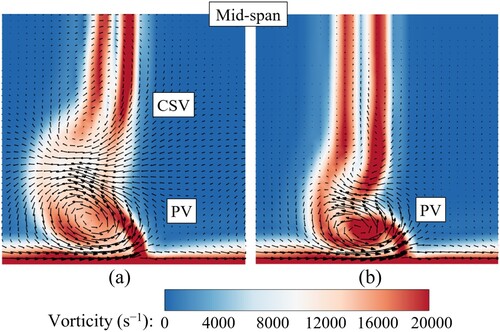
Figure 38 shows the transient distribution of the endwall flow, injection flow and axial vorticity at the 150% axial chord section at 10T/20. It can be seen that the endwall low-momentum fluid was divided into two branches at the injection location, which were denoted as Branch-A (green lines) and Branch-B (orange lines). Regarding the effect of injection fluid with high momentum, Branch-A migrated to a higher cascade span and Branch-B still flowed near the endwall. Compared with the Mid-PEAI case, Branch-B of the Trail-PEAI case reduced significantly, indicating that more endwall low-momentum fluid migrated toward the mid-span. Therefore, an injection location closer to the trailing edge can effectively suppress the development of the passage vortex. According to the distribution of streamlines of injection flow, the spanwise velocity of the injection fluid decreased as it flowed downstream. Compared with the other cases, the injection fluid of the Trail-PEAI case exhibited higher spanwise momentum when reaching the trailing edge, so most of the streamlines of the injection fluid accumulated near 30–40% cascade span, and more low-momentum fluid migrated to the mid-span. The more spanwise migration of low-momentum fluid for the Trail-PEAI case caused a decrease in the concentrating shedding vortex (Figure 36b) and an increase in the trailing edge separation (Figure 35b).

Figure 38. Transient distribution of endwall flow and injection flow at different pulsed endwall air injection (PEAI) locations (t = 10T/20): (a) Mid-PEAI case; (b) Trail-PEAI case. CSV = concentrating shedding vortex; PV = passage vortex.

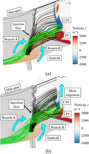
Figure 39 shows the transient vortex structure and distribution of injection flow at 10/20T under different injection locations. Since the injection fluid of the Lead-PEAI case affected more regions in the suction corner, the spanwise velocity component of the injection fluid was much less than in the other PEAI cases. Therefore, less low-momentum fluid migrated to the mid-span, which can be seen from the streamwise vortex in Figure 39(a). As a result, there was no injection vortex near the mid-span but there was a larger hairpin vortex. In Figure 39(b), the injection vortex appeared at the mid-span; its formation mechanism has been explained in Section 5.1. The intensity of the hairpin vortex was obviously suppressed and the concentrating shedding vortex was eliminated by the Trail cascade.

Figure 39. Transient vortex structures and injection flow distribution at different pulsed endwall air injection (PEAI) locations (t = 10T/20, Q = 5 × 10⁵ s⁻²): (a) Lead-PEAI case; (b) Trail-PEAI case. PV = passage vortex; CSV = concentrating shedding vortex.

5.5. Effect of injection hole diameter on PEAI

In previous subsections from Section 5.1 to Section 5.4, the injection hole diameter of all PEAI cases was set to 4 mm. To reveal the effect of injection hole diameter on the flow field of PEAI cascades, PEAI cases with different injection hole diameters (3 and 5 mm) are investigated in this subsection. Under the injection amplitude of 1.22, injection frequency of 0.975 and injection location at the 74.1% axial chord, PEAI cases with different injection hole diameters (3 and 5 mm) are investigated in this subsection.

Figure 40 shows the time-averaged cascade loss coefficient, overall loss coefficient and endwall loss coefficient of SEAI cases and PEAI cases with different injection hole diameters. From Figure 40(a), the cascade loss of all injection cases increased with the increase in the injection hole diameter, and there was little difference between PEAI cases and SEAI cases. Considering the injection loss in Figure 40(b), the larger injection hole diameter led to a greater injection loss, and the PEAI case with the injection hole diameter of 3 mm exhibited the lowest overall loss coefficient. In Figure 40(c), in contrast to the results for injection amplitudes in Section 5.2, the endwall losses of PEAI cases were almost unchanged, whereas the endwall loss of SEAI cases increased with the increase in injection hole diameter, which meant that variation of the injection hole diameter did not simply affect the flow field by changing the injection mass flow rate.

Figure 40. Variation of loss coefficients under different injection hole diameters (St = 0.975, $\overline{A}$ = 1.22): (a) time-averaged cascade loss coefficient; (b) time-averaged overall loss coefficient; (c) time-averaged endwall loss coefficient. SEAI = steady endwall air injection; PEAI = pulsed endwall air injection.

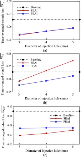
Figure 41 shows the spanwise distribution of the time-averaged local loss coefficients of SEAI and PEAI cases with different injection hole diameters. According to the figure, the injection hole diameter mainly affected the local loss coefficients ranging from 0% to 15% blade span and from 25% to 50% blade span. The case with a larger injection hole diameter exhibited higher losses near the endwall and mid-span, especially in the SEAI case.

Figure 41. Time-averaged local loss coefficient distribution along spanwise at 150% relative axial chord (St = 0.975, $\overline{A}$ = 1.22): (a) steady endwall air injection (SEAI) cases; (b) pulsed endwall air injection (PEAI) cases.

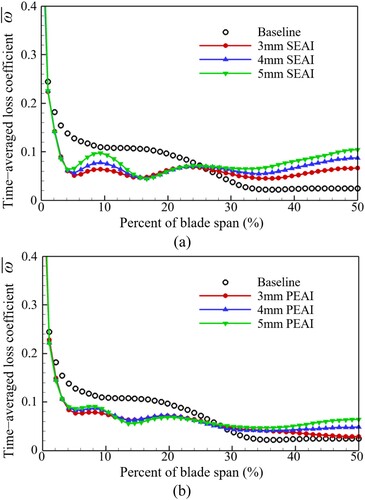
Figure 42 shows the time-averaged secondary flows and vorticity magnitude contours at the 150% axial chord of SEAI and PEAI cases with different injection hole diameters. It can be seen that the vorticity magnitude near the endwall and the intensity of the passage vortex were obviously increased with the increase in the injection hole diameter. Compared with the other cases, the concentrating shedding vortex of the PEAI case with an injection hole diameter of 3 mm (Figure 42c) exhibited the largest spanwise distribution range. When injection hole diameter increased to 5 mm, because plenty of low-momentum fluid migrated toward the mid-span, the injection vortex appeared at the mid-span.

Figure 42. Time-averaged secondary flow and vorticity contours at 150% relative axial chord with different injection hole diameters (St = 0.975, $\overline{A}$ = 1.22): (a) steady endwall air injection (SEAI) (3 mm); (b) SEAI (5 mm); (c) pulsed endwall air injection (PEAI) (3 mm); (d) PEAI (5 mm). CSV = concentrating shedding vortex; PV = passage vortex.

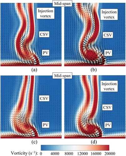
Figure 43 shows the transient vortex structure and distribution of injection flow of PEAI cases at 10T/20 with different injection hole diameters. For the case with an injection hole diameter of 3 mm in Figure 43(a), most of the injection fluids were distributed near the endwall, and a branch of injection fluid ranging near 40% blade span enlarged the spanwise scale of the concentrating shedding vortex. For the case with the injection hole diameter of 5 mm, the transient flow field was similar to the flow field of the PEAI case (St = 0.975, $\overline{A}$ = 1.40 and injection hole diameter of 4 mm), as shown in Figure 24(c). The excess injection fluid strengthened the intensity of the vortices in the cascade passage, which brought about the extra loss.

Figure 43. Transient vortex structures and distributions of injection flow with different injection hole diameters (t = 10T/20, $\overline{A}$ = 1.22, Q = 5 × 10⁵ s⁻²): (a) pulsed endwall air injection (PEAI) (3 mm); (b) PEAI (5 mm). PV = passage vortex; CSV = concentrating shedding vortex.

6. Conclusions and prospects

In this study, PEAI was numerically carried out in a compressor cascade, and the mechanisms through which it influenced corner separation and the vortex structure were revealed. The effects of PEAI parameters (injection amplitude, injection frequency, injection location and diameter of the injection hole) were also investigated. Conclusions are drawn as follows:

1. PEAI can effectively suppress the 3D corner separation. The optimal control scheme reduced the time-averaged overall loss coefficient by 10.5%, with the relative injection amplitude of 1.22 and St of 0.975, which showed that PEAI had a better control effect than SEAI under the same injection amplitude. Low-momentum fluid migrated toward the mid-span after applying PEAI, which deteriorated the flow field at mid-span. Regarding the effect of PEAI, the interaction between the passage vortex and concentrating shedding vortex resulted in the formation of a hairpin vortex. The accumulated low-momentum fluid at mid-span rolled up the injection vortex because of the spanwise expanded concentrating shedding vortex.

2. As the injection amplitude increased, the area of the reverse flow region in the suction corner gradually disappeared. Under a low injection amplitude, the effect of PEAI was confined to a limited area. Since the injection amplitude was too weak to provide enough energy for the low-momentum fluid in the suction corner, plenty of low-momentum fluid migrated toward the 30–40% blade span, which resulted in an increase in the concentrating shedding vortex. Under a high injection amplitude, the flow field near the mid-span was deteriorated owing to the spanwise migration of low-momentum fluid. The interaction among trailing edge separation, low-momentum fluid near the mid-span and the spanwise expanded concentrating shedding vortex led to the formation of an obvious injection vortex when the injection amplitude was 1.40.

3. When conducting PEAI, the effect of inertia existed for the flow in the injection hole. Under low St (0.002), the length of a single time step was long enough to allow injection fluid to flow across the injection hole, so the effect of inertia was extremely weak. Therefore, in the PEAI case with a sufficiently small St, the effect of the initial injection phase on the baseline flow field could be clearly observed. The injection vortex was found near the mid-span at time 15T/20 and then disappeared as the injection flow significantly declined during the remaining injection period. Under high injection frequency, the variation of flow fields at different times was moderate because of the strong effect of inertia. The periodic injection led to a series of hairpin vortices distributed at equal intervals.

4. Unlike the SEAI cases, the PEAI case with further downstream injection location featured lower endwall loss. The injection scheme of the Trail-PEAI case directly controlled the concentrating shedding vortex. The injection hole location of PEAI affected the flow field by changing the effect region of the injection and low-momentum fluid near the endwall. As the injection hole location moved downstream, the corner separation line migrated toward the trailing edge, and the injection fluid featured more spanwise momentum at the trailing edge, which led to more endwall low-momentum fluid accumulating toward the mid-span. Meanwhile, the injection location close to the trailing edge reduced the endwall fluid forming the passage vortex, which suppressed the endwall loss. In addition, the injection vortex was found in the transient flow field of the Trail-PEAI case.

5. The variation of injection hole diameter did not simply affect the flow field by changing the injection mass flow rate. The injection hole diameter had a significant impact on the intensity of the passage vortex and mid-span flow field. As the injection hole diameter increased, the intensity of the passage vortex increased and the mid-span flow field deteriorated.

In this work, PEAI was preliminarily investigated in a compressor cascade, and achieved an excellent control effect on flow separation with a lower injection mass flow rate. However, in the actual multi-stage axial compressor, the unsteady effect, especially the blade wake from the upstream blades, could be regarded as an unsteady actuator in a compressor, so it must be considered. In this condition, the injection frequency is a decisive factor affecting the effectiveness of PEAI, and the interaction effect between the unsteady inflow and PEAI needs to be determined. The authors are investigating the effect of PEAI on compressor blades under the actual multi-stage axial compressor, and relevant research results will be presented in another manuscript in the near future.

Acknowledgement

This work was supported by the National Natural Science Foundation of China (number 51806174), National Science and Technology Major Project (number J2019-II-0011-0031), and National Natural Science Foundation of China (number 51790512).

Disclosure statement

No potential conflict of interest was reported by the authors.

Additional information

Funding

This work was supported by the National Natural Science Foundation of China [grant numbers 51790512 and 51806174]; National Major Science and Technology Projects of China [grant number J2019-II-0011-0031].

Appendix

Notation

$\overline{A}$	=	Injection amplitude
C	=	Chord
Ca	=	Axial chord
Cp	=	Static pressure coefficient
Cp	=	Specific heat capacity
D	=	2D diffusion factor
f	=	Injection frequency
h	=	Blade height
m	=	Mass flow rate
Ma1	=	Inlet Mach number
P	=	Static pressure
P*	=	Total pressure
Q	=	Q-criterion
R	=	Specific gas constant
Re	=	Reynolds number
S	=	Shear strain rate tensors
St	=	Strouhal number
t	=	Time
T	=	Period of pulsed endwall air injection
T*	=	Total temperature
v	=	Velocity
x	=	Spanwise coordinate
y	=	Pitchwise coordinate
z	=	Axial coordinate
β1	=	Inflow angle
β2	=	Outflow angle
βk	=	Stagger angle
Δs	=	Entropy generation
ρ	=	Density
τ	=	Solidity of cascade
Ω	=	Vorticity
ω	=	Local loss coefficient
ωca	=	Cascade loss coefficient
ωet	=	Overall loss coefficient
ωew	=	Endwall loss coefficient

Subscripts

1	=	Inlet boundary of the cascade
2	=	150% axial chord section
jet	=	Injection inlet boundary
local	=	Local value
z	=	Axial

Abbreviations

CSL	=	Corner separation line
CSV	=	Concentrating shedding vortex
CV	=	Corner vortex
HP	=	Pressure surface side leg of horseshoe vortex
HS	=	Suction surface side leg of horseshoe vortex
LE	=	Blade leading edge
PEAI	=	Pulsed endwall air injection
PV	=	Passage vortex
SEAI	=	Steady endwall air injection
TE	=	Blade trailing edge
TSL	=	Trailing separation line

References

- Brück, C., Tiedemann, C., & Peitsch, D. (2016). Experimental investigation on highly loaded compressor airfoils with active flow control under non-steady flow conditions in a 3D-annular low-speed cascade. ASME Turbo Expo 2016: Turbomachinery Technical Conference and Exposition (ASME paper no. GT2016-56891).
- Bryce, J. D., Cherrett, M. A., & Lyes, P. A. (1995). Three-dimensional flow in a highly loaded single-stage transonic fan. Journal of Turbomachinery, 117(1), 22–28. https://doi.org/10.1115/1.2835640
- Bullock, R. O., & Johnsen, I. A. (1965). Aerodynamic design of axial-flow compressors. NASA (NASA Report No. SP-36).
- Cao, Z. Y., Gao, X., & Liu, B. (2021). Influence of endwall Air injection with discrete holes on corner separation of a compressor cascade. Journal of Thermal Science, 30(5), 1684–1704. https://doi.org/10.1007/s11630-021-1513-5
- Cao, Z. Y., Liu, B., & Zhang, T. (2014). Control of separations in a highly loaded diffusion cascade by tailored boundary layer suction. Proceedings of the Institution of Mechanical Engineers, Part C: Journal of Mechanical Engineering Science, 228(8), 1363–1374. https://doi.org/10.1177/0954406213508281
- Cao, Z. Y., Zhou, C., & Sun, Z. L. (2017). Comparison of aerodynamic characteristics between a novel highly loaded injected blade with curvature induced pressure-recovery concept and one with conventional design. Chinese Journal of Aeronautics, 30(3), 939–950. https://doi.org/10.1016/j.cja.2017.03.018
- Chen, J., Lu, W. Y., Huang, G. P., Zhu, J. F., & Wang, J. C. (2017). Numerical simulation and experimental verification of suppressing flow separation in a cascade by pulsed jet without external energy injection. 53rd AIAA/SAE/ASEE Joint Propulsion Conference (AIAA Paper No. AIAA 2017-4732).
- Culley, D. E., Bright, M. M., Prahst, P. S., & Strazisar, A. J. (2004). Active flow separation control of a stator vane using embedded injection in a multistage compressor experiment. Journal of Turbomachinery, 126(1), 24–34. https://doi.org/10.1115/1.1643912
- Estevadeordal, J., Koch, P., Guillot, S., Ng, W., Car, D., & Puterbaugh, S. (2004). Benefits of suction-surface blowing in a transonic compressor stator vane. 2nd AIAA Flow Control Conference (AIAA Paper No. AIAA 2004-2207).
- Evans, S., Coull, J., Haneef, I., & Hodson, H. (2012). Minimizing the loss produced by a turbulent separation using vortex generator jets. AIAA Journal, 50(4), 778–787. https://doi.org/10.2514/1.J050790
- Evans, S., & Hodson, H. (2011). The cost of flow control in a compressor. ASME 2011 Turbo Expo: Turbine Technical Conference and Exposition (ASME paper No. GT2011-45059).
- Gbabebo, S. A., Cumpsty, N. A., & Hynes, T. P. (2005). Three-dimensional separations in axial compressors. Journal of Turbomachinery, 127(2), 331–339. https://doi.org/10.1115/1.1811093
- Ghalandari, M., Ziamolki, A., Mosavi, A., Shamshirband, S., & Chau, K. W. (2019). Aeromechanical optimization of first row compressor test stand blades using a hybrid machine learning model of genetic algorithm, artificial neural networks and design of experiments. Engineering Applications of Computational Fluid Mechanics, 13(1), 892–904. https://doi.org/10.1080/19942060.2019.1649196
- Gmelin, C., Steger, M., Thiele, F., Thielex, F., Huppertz, A., & Swoboda, M. (2010). Unsteady RANS simulations of a highly loaded low aspect ratio compressor stator cascade with active flow control. ASME Turbo Expo 2010: Power for Land, Sea, and Air (ASME paper no. GT2010-22516).
- Gmelin, C., Zander, V., Hecklau, M., Thiele, F., Nitsche, W., Huppertz, A., & Swoboda, M. (2012). Active flow control concepts on a highly loaded subsonic compressor cascade: Résumé of experimental and numerical results. Journal of Turbomachinery, 134(6), 061021. https://doi.org/10.1115/1.4006308
- Hecklau, M., Wiederhold, O., Zander, V., King, R., Nitsche, W., Huppertz, A., & Swoboda, M. (2011). Active separation control with pulsed jets in a critically loaded compressor cascade. AIAA Journal, 49(8), 1729–1739. https://doi.org/10.2514/1.J050931
- Hunt, J. C. R., Wray, A. A., & Moin, P. (1988). Eddies streams and convergence zones in turbulent flows. Technical Report CTR-S88, Center for Turbulence Research.
- Kan, X. X., Wu, W. Y., & Zhong, J. J. (2020). Effects of vortex dynamics mechanism of blade-end treatment on the flow losses in a compressor cascade at critical condition. Aerospace Science and Technology, 102, 105857. https://doi.org/10.1016/j.ast.2020.105857
- Li, L. T., Song, Y. P., Chen, F., & Liu, H. P. (2016). Flow control investigations of steady and pulsed jets in bowed compressor cascades. ASME Turbo Expo 2016: Turbomachinery Technical Conference and Exposition (ASME paper no. GT2016-56855).
- Meng, Q. H., Chen, S. W., Li, W. H., & Wang, S. T. (2018). Numerical investigation of a sweeping jet actuator for active flow control in a compressor cascade. ASME Turbo Expo 2018: Turbomachinery Technical Conference and Exposition (ASME paper no. GT2018-76052).
- Nerger, D., Saathoff, H., Radespiel, R., Gummer, V., & Clemen, C. (2012). Experimental investigation of endwall and suction side blowing in a highly loaded compressor stator cascade. Journal of Turbomachinery, 134(2), 021010. https://doi.org/10.1115/1.4003254
- Rivir, R. B., Sondergaard, R., Bons, J. P., & Lake, J. P. (2000). Passive and active control of separation in gas turbines. Fluids 2000 Conference and Exhibit (AIAA paper no. AIAA 2000-2235).
- Salih, S. Q., Aldlemy, M. S., Rasani, M. R., Ariffin, A. K., Ya, T. M. Y. S. T., Al-Ansari, N., Yaseen, Z. M., & Chau, K. W. (2019). Thin and sharp edges bodies-fluid interaction simulation using cut-cell immersed boundary method. Engineering Applications of Computational Fluid Mechanics, 13(1), 860–877. https://doi.org/10.1080/19942060.2019.1652209
- Sarimurat, M. N., & Dang, T. Q. (2014). An analytical model for boundary layer control via steady blowing and its application to NACA-65-410 cascade. Journal of Turbomachinery, 136(6), 061011. https://doi.org/10.1115/1.4025585
- Staats, M., & Nitsche, W. (2016). Active control of the corner separation on a highly loaded compressor cascade with periodic non-steady boundary conditions by means of fluidic actuators. Journal of Turbomachinery, 138(3), 031004. https://doi.org/10.1115/1.4031934
- Staats, M., & Nitsche, W. (2017). Experimental investigations on the efficiency of active flow control in a compressor cascade with periodic non-steady outflow conditions. ASME Turbo Expo 2017: Turbomachinery Technical Conference and Exposition (ASME paper no. GT2017-63246).
- Sun, S. J., Wang, S. T., Zhang, L. X., & Ji, L. C. (2021). Design and performance analysis of a two-stage transonic low-reaction counter-rotating aspirated fan/compressor with inlet counter-swirl. Aerospace Science and Technology, 111, 106519. https://doi.org/10.1016/j.ast.2021.106519
- Tang, Y. M., Liu, Y. W., Lu, L. P., Lu, H. W., & Wang, M. (2019). Passive separation control with blade-end slots in a highly loaded compressor cascade. AIAA Journal, 58(1), 85–97. https://doi.org/10.2514/1.J058488
- Taylor, J. V., & Miller, R. B. (2017). Competing three-dimensional mechanisms in compressor flows. Journal of Turbomachinery, 139(2), 021009. https://doi.org/10.1115/1.4034685
- Tiedemann, C., Heinrich, A., & Peitsch, D. (2012). A new linear high speed compressor stator cascade for active flow control investigations. 6th AIAA Flow Control conference (AIAA paper no. 2012-3251).
- Wennerstrom, A. J. (1990). Highly loaded axial flow compressors: History and current developments. Journal of Turbomachinery, 112(4), 567–578. https://doi.org/10.1115/1.2927695
- Young, J. B., & Horlock, J. H. (2006). Defining the efficiency of a cooled turbine. Journal of Turbomachinery, 128(4), 658–667. https://doi.org/10.1115/1.2218890
- Zhang, H. D., Wu, Y., Li, Y. H., Yu, X. J., & Liu, B. J. (2019). Control of compressor tip leakage flow using plasma actuation. Aerospace Science and Technology, 86, 244–255. https://doi.org/10.1016/j.ast.2019.01.009
- Zheng, X. Q., Zhang, Y. J., Xing, W. D., & Zhang, J. Y. (2011). Separation control of axial compressor cascade by fluidic-based excitations. Journal of Turbomachinery, 133(4), 041016. https://doi.org/10.1115/1.4002407
- Zheng, X. Q., Zhou, S., Hou, A. P., Jiang, Z. L., & Ling, D. J. (2006). Separation control using synthetic vortex generator jets in axial compressor cascade. Acta Mechanica Sinica, 22(6), 521–527. https://doi.org/10.1007/s10409-006-0042-5
- Zheng, X. Q., Zhou, X. B., & Zhou, S. (2005). Investigation on a type of flow control to weaken unsteady separated flows by unsteady excitation in axial flow compressors. Journal of Turbomachinery, 127(3), 489–496. https://doi.org/10.1115/1.1860572
- Zhong, L. X., Zhou, C., & Chen, S. Y. (2016). Effects of approaching main flow boundary layer on flow and cooling performance of an inclined jet in cross flow. International Journal of Heat and Mass Transfer, 103: 572-581. https://doi.org/10.1016/j.ijheatmasstransfer.2016.07.089