Hydrodynamic numerical simulation and prediction of bionic fish based on computational fluid dynamics and multilayer perceptron

ABSTRACT

This paper proposes a prediction strategy for the hydrodynamic performance of bionic fish. The major challenges are meshing and building prediction model. The NACA0012 airfoil is used to replace the fish driven by the body and/or caudal fin (BCF), and a two-dimensional swimming geometric model is constructed. The geometric model is divided into hybrid meshes using the overset mesh method. The classical traveling wave model is studied using Matlab, and an improved self-propelled motion model is established. The hydrodynamic performance of the self-propelled model is numerically simulated based on computational fluid dynamics (CFD). In this strategy, the geometric model and the self-propelled motion model are integrated with user defined functions (UDF). The influences of the parameters such as inflow velocity, frequency, wavelength, and head fluctuation amplitude on the motion performance are studied. The results show that when inflow velocity is uniform, the self-propelled motion will eventually reach a quasi-steady state. According to the numerical simulation results, a hydrodynamic performance prediction model is established based on multilayer perceptron (MLP). The model is used to predict the performance of the optimized traveling wave parameters, and the error is within 3$\mathrm{\%}$. The accuracy and generalization ability of the MLP prediction model is verified.

KEYWORDS:

• Bionic fish
• traveling wave
• self-propelled model
• computational fluid dynamics
• multilayer perceptron

1. Introduction

After millions of years of evolution, fish demonstrates superior hydrodynamic performance and high movement efficiency. In addition, 85$\mathrm{\%}$ of fish are driven by the body and/or caudal fin (BCF). Studies have shown that the flapping and wave propulsion methods of most fish are generally more efficient than conventional propellers. Compared with traditional autonomous underwater vehicles (AUVs), the bionic robotic fish has better mobility, flexibility, and concealment. Many scholars at home and abroad have never interrupted their research on bionic fish.

Lighthill (1960) expounded the slender body theory for the first time, established a traveling wave model, and laid the foundation for subsequent research. Videler and Hess (1984) proposed a kinematic analysis method and analyzed the continuous swimming of fish. C. Zhou et al. (2008) analyzed the propulsion generated by the tail wave and modified the swimming law of robotic fish. Guang et al. (2014) proposed a circle threshold interval discretion (CTID) method to fit the traveling wave of a bionic robotic fish. Scaradozzi et al. (2017) reviewed the research process of bionic robotic fish and applied the cam-like mechanism to move closer with the traveling wave formula. Cui et al. (2018) studied the swimming of the fish's midline and analyzed the traveling waves using the traveling index. H. Liu and Curet (2018) conducted theoretical analysis and experimental research on the swimming performance of the wave-fin propelled bionic robotic fish. Thekkethil et al. (2018) used a general kinematic model to study various types of fluctuations in fluid dynamics. Gibouin et al. (2018) studied the characteristics of thrust and resistance and their balance when swimming with a bionic robotic fish. Tanha and Feeny (2019) derived the properties of traveling wave and evaluated the accuracy of traveling wave model. Xie et al. (2019) studied the influence of the fish body wave mode on the cruise performance and analyzed the thrust, cruise speed, and swimming efficiency using traveling wave model. The above references carried out abundant theoretical research and experimental analysis on traveling wave model, but no optimization strategy was proposed.

It can be seen from traveling wave model that amplitude, wavelength, and frequency are the main parameters that affect wave pattern. With the gradual improvement of computer performance, it is more and more convenient to use computational fluid dynamics (CFD) to study the swimming performance of bionic fish. The immersed boundary method (IBM) has been widely used (Cui et al., 2017; Han et al., 2020; Khalid et al., 2018; G. Liu et al., 2017; Salih et al., 2019; Tytell et al., 2010; Wang & Wu, 2010; Zhang et al., 2018). Using IBM can improve efficiency.

In addition, Yong-hua et al. (2007) employed the CFD method to analyze the thrust and efficiency of the wave-like bionic fish under different swimming models. H. Zhou et al. (2010) numerically simulated the wave propulsion scheme through a two-dimensional model. Chang et al. (2012) used a dynamic hybrid mesh method to numerically simulate fish swimming patterns under different Reynolds numbers ($\mathrm{R}\mathrm{e}$). Ji and Huang (2017) carried out a numerical simulation on the influence of $\mathrm{R}\mathrm{e}$ on energy extraction efficiency of the wave flexible model. Ming et al. (2019) coupled the three-dimensional CFD model to the motion of fish, calculated the distribution of torque and power. Zhao and Dou (2019a) carried out a numerical simulation on the combined undulating-motion pattern (CUMP) of bionic fish. They also studied the effects of spatial distance between the undulating foil and the flapping foil on the propulsive performance. R. Li et al. (2020) combined CFD and multi-body dynamics (MBD) to study the self-propelled motion of fish in the acceleration and quasi-steady state phases. Gao et al. (2021) used grid deformation technology to simulate the hydrodynamic performance of traveling waves numerically. Tian (2020) used the Deforming-Spatial-Domain/Stabilize-Space-Time (DSD/SST) method to study the hydrodynamic mucus effects of the two-dimensional fish model. Sun et al. (2020) established a simplified two-dimensional model and studied the influence of the shape of the leading edge on the hydrodynamic characteristics of wave airfoil based on CFD. Ma et al. (2021) used NACA0012 airfoil to create a simplified two-dimensional model, studied the effect of spacing and phase difference on the energy harvesting of dual wave airfoils based on numerical simulation. The references cited in this paragraph studied the impact of boundary conditions and traveling wave parameters on hydrodynamic performance based on CFD. However, the corresponding mapping relationship and optimization model were not established.

Machine learning provides a wealth of technology to extract and process data and has been widely used in fluid mechanics and engineering (Brunton et al., 2020). Gazzola et al. (2014) proposed a numerical simulation method for self-propelled swimming based on reinforcement learning. H. Zhou et al. (2015) established the mapping relationship between the inlet velocity and the near-body pressure under different fluctuation parameters based on CFD and a filtering algorithm. Novati et al. (2017) optimized the cooperative swimming mode of two self-propelled bionic fish based on reinforcement learning. Xu et al. (2017) obtained the pressure simulation data of the bionic fish swimming flow field based on CFD and classified the flow field using a back-propagation neural network (BPNN). Colvert et al. (2018) classified the wake vortices of bionic fish swimming based on a neural network. Based on CFD numerical simulation and machine learning, S. Li et al. (2019) established the flow velocity prediction model and spacing judgment model of the bionic fish formation. Shen et al. (2020) established a genetic algorithm back-propagation neural network (GA-BPNN) model to predict the velocity of a hybrid robotic fish (HRF) driven by waves and sails. Based on CFD and deep reinforcement learning methods, Yan et al. (2020) established a hydrodynamic/kinematic/motion-control coupling model to study the self-propelled swimming of bionic fish. Dong et al. (2021) optimized the gliding efficiency of robotic fish based on deep reinforcement learning. Huang et al. (2021) studied the drag reduction of underwater series multiple bombs based on CFD and machine learning and established a drag coefficient prediction model using simulation data. Kochkov et al. (2021) improved the numerical simulation of two-dimensional turbulence in CFD based on deep learning. N. Li et al. (2021) optimized the lightweight design parameters of the AUV pressure hull based on BPNN. Although the above scholars have carried out much analysis on the swimming of bionic fish based on CFD and machine learning, the optimization of traveling wave parameters and the prediction of hydrodynamic performance of self-propelled motion still need continuous and in-depth research.

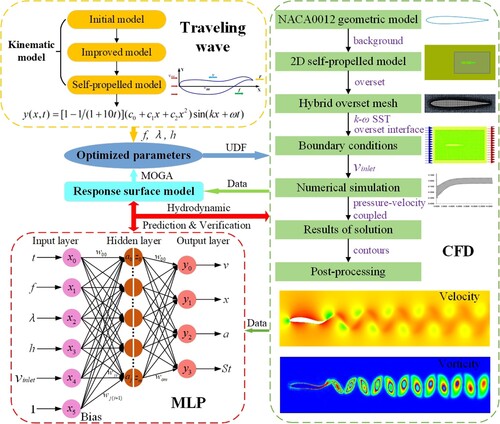
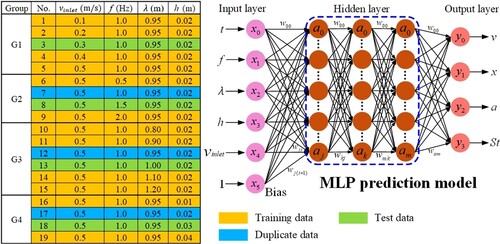
A novel hydrodynamic prediction strategy is proposed based on CFD and multilayer perceptron (MLP), as shown in Figure 1. The major challenges are meshing and building prediction model. A two-dimensional self-propelled motion model driven by user defined functions (UDF) is established. Numerical simulations are performed on the motion performance under different parameters, and the simulation results are used as a data set to construct a hydrodynamic prediction model. The results show that the prediction effect of the model is superior, and the reliability of the prediction strategy is verified. This paper consists of 6 sections: the research process of bionic fish is introduced in Section 1; the classic traveling wave model and improved self-propelled model are described in Section 2; the overset mesh, numerical simulation method, and boundary conditions are introduced in Section 3; the results of the numerical simulation are discussed in Section 4; a hydrodynamic prediction model is established based on MLP, and the predicted results are verified in Section 5; the conclusions and prospect are given in Section 6. Combining CFD and MLP to make hydrodynamic predictions for bionic fish is the original achievement of this paper.

Figure 1. Hydrodynamic numerical simulation and prediction strategy.

2. Kinematic model optimization

2.1. Kinematic model of traveling wave

The motion of fish can be expressed as a propulsion wave with increasing amplitude (Cui et al., 2018). In the 1960s, Lighthill proposed a classic traveling wave kinematic model, which is expressed as follows: (1) $\{\begin{array}{l}y(x,t)=(c_{1}x+c_2{x}^2)\sin (kx+\omega t)\\ k={\displaystyle \frac{2\pi }{\lambda }}\\ \omega =2\pi f\end{array}$(1) where y is the lateral fluctuation displacement; x is the displacement along the axial direction; t is time; $c_1$ and $c_2$ are the coefficients of linear amplitude envelope and quadratic envelope, respectively; k is the wavenumber of the traveling wave; λ represents the wavelength; f represents the frequency of fluctuations.

This model describes the ideal swimming pattern of a bionic fish, assuming that the head is rigid and does not swing to the sides of the x-axis. Although the motion of bionic fish is very realistic, its performance is still very different from that of the fish. When a fish swims, the head swing caused by inertia and reaction force can be restrained by biological function. When a bionic fish swims, inertia and reaction forces also exist. In addition, with the influence of fish body size, proportion configuration, and processing errors, the head swing cannot be eliminated entirely. Therefore, using the above kinematic model to describe the motion of bionic fish is not completely accurate.

After that, researchers modified the model to translate fish's swimming as a function of tail movement relative to head (Gao et al., 2021; J. Liu & Hu, 2010). The improved model is expressed as follows: (2) $f_T(x,t)=(c_{1}x+c_2{x}^2)\sin (kx+\omega t)-c_{1}x\sin \left(\omega t\right)$(2) where $c_1\sin \left(\omega t\right)$ is the first derivative of $y(x,t)$ at x = 0. The results show that the improved model has superior propulsion performance. However, the improved model does not have a self-propelled effect. It does not show a process from static to acceleration and then to stability.

2.2. Self-propelled kinematic model

In this paper, considering the small swing of the head of bionic fish, the initial model is optimized, and a constant term is added to the amplitude envelope (Cui et al., 2017, 2018; Khalid et al., 2018; Wang & Wu, 2010). In order to realize the self-propelled motion launching at t = 0, the time coefficient is added in front of the traveling wave function. It is clear that bionic fish does not swim when t = 0. As time goes on, the time coefficient gets closer to 1. That is to say, the time coefficient works mainly at the initial moment of launch. The optimized self-propelled model is expressed as follows: (3) $\begin{array}{rl}y(x,t)& =[1-1/(1+10t\left)\right](c_0+c_{1}x+c_2{x}^2)\\ & \times \sin (kx+\omega t)\end{array}$(3) where $1-1/(1+10t)$ is the time coefficient; $c_0$ is the constant term of the envelope. In order to facilitate the comparison between the research results and the references, the initial values of the self-propelled kinematic model refer to the references above (Wang & Wu, 2010; Zhao & Dou, 2019b). We assume that the total length of bionic fish is 1 m, and define $c_0=0.02$, $c_1=-0.08$, $c_2=0.16$, $\lambda =0.95\mathrm{m}$, and f = 1.0 Hz.

The self-propelled model indicates that bionic fish starts to swim at t = 0, and the body and tail wave generate the thrust. The forward acceleration, velocity, and displacement are calculated in real-time according to the thrust at different moments. With the increase of velocity, the resistance improves until the thrust and resistance are in a dynamic balance, and the swimming reaches a quasi-steady state. The coordinate system and variables of the self-propelled model are shown in Figure 2, and the calculation formula is expressed as follows: (4) $\{\begin{array}{l}{a}_i=-{\displaystyle \frac{F_i-f_i}{m}}\\ v_{i+1}=v_i+{\displaystyle \frac{a_i+a_{i+1}}{2}}dt\\ d{x}_{i+1}={\displaystyle \frac{v_i+v_{i+1}}{2}}dt\\ x_{i+1}=x_i+d{x}_{i+1}\\ i=0,1,2,3\dots \dots \end{array}$(4) where $F_i$ is the thrust generated by bionic fish at point i; $f_i$ is the resistance at point i; m is the weight of bionic fish; $a_i$ is the acceleration at point i; $v_i$ is the velocity along the x-axis at point i; x represents the displacement along the x-axis; dt and dx represent time and displacement increment, respectively. Based on Matlab, the initial model, the improved model, and the self-propelled model are simulated and analyzed, and the analysis results are shown in Figure 3.

Figure 2. Self-propelled model coordinate system and variables.

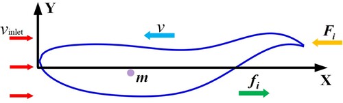
Figure 3. The posture analysis of the three models at different moments: (a) The initial model, (b) The improved model, (c) The self-propelled model, (d) t = 0.25 s, (e) t = 0.5 s, (f) t = 0.75 s.

In Figure 3(a–c) respectively represent the initial model, the improved model, and the self-propelled model. The upper figure shows the posture of bionic fish at different moments, and the lower figure shows the traveling waves at different moments in a cycle. In the initial model, there is no fluctuation in the head and middle part of the body, while the fluctuation in the back and tail of the body is significant. In the improved model, the head does not fluctuate. The front and tail of the body fluctuate slightly, and the back of the body fluctuates more obviously. However, in the self-propelled model, there is a slight fluctuation of the head and the front of the body and an extensive fluctuation of the back and tail of the body. The detailed difference of the three models at different moments are shown in Figure 3(d–f). The self-propelled model is similar to the initial model's wave pattern and significantly differs from the improved model. However, the difference in the maximum fluctuation amplitude of the three models is not obvious. At the moment of t = 0.5, the traveling waves of the initial model and the improved model are consistent. In Figure 3(e), the green line and the red line completely coincide. In summary, the motion posture simulation shows that the self-propelled model is more consistent with the swimming mode of bionic fish.

3. Numerical simulation

In this paper, NACA0012 airfoil is used as geometric model. Firstly, overset mesh method is used to divide bionic fish and fluid zones. Then bionic fish swimming mode and boundary conditions are customized through UDF, and numerical simulation is conducted based on Fluent. Finally, the simulation results are post-processed and analyzed by Tecplot. Two-dimensional modeling and numerical simulation are carried out on the ASUS ExpertCenter D5 Tower desktop computer. The computer is configured with 16-core Intel(R) Core(TM) i7-10700 CPU @2.90 GHz and 32.0 GB RAM.

3.1. Geometric model

The NACA0012 airfoil is widely used because of its superior hydrodynamic performance and similar appearance to the fish body (Khalid et al., 2018; Thekkethil et al., 2018). NACA0012 airfoil is also applied as the fish body in this paper, and the total length (L) of the fish is 1 m. Taking the airfoil chord length as the midline of the fish body, the amplitude of the lateral fluctuation is described by a quadratic function, as shown below: (5) $\{\begin{array}{l}h\left(x\right)=c_0+c_{1}x+c_2{x}^2\\ 0\le x\le 1\end{array}$(5) The self-propelled model studied in this paper only involves axial movement and lateral fluctuations. When x approaches 0, h represents the fluctuation amplitude of the head. It is worth mentioning that the back of the NACA airfoil curve is not closed. After importing to SolidWorks, the curve is manually repaired. We use an arc with a radius of 3 mm to connect the upper and lower edges, and the two-dimensional model is generated, as shown in Figure 4.

Figure 4. The two-dimensional geometric model.

3.2. Overset mesh

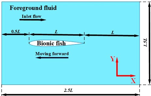
The geometric model is established in SolidWorks and DesignModeler, and then set up progressively based on ANSYS Workbench. After the model is created, the overset mesh (Broniszewski & Piechna, 2019; Dai et al., 2021; Kandula et al., 2008; Shi et al., 2017; Su et al., 2019; Yao et al., 2020) is divided. Overset mesh can simplify the meshing of complex geometries and facilitate the generation of meshes for relatively moving parts. In addition, the overset mesh is adopted to deal with dynamic mesh problems, which facilitates the solution of negative volume of the dynamic mesh. In this paper, the foreground component is meshed firstly. The foreground area is $2.5L\times 1.5L$, and the size of the surface mesh is set to 20 mm. The size of the edge line and the fish contour line in the foreground area are defined, respectively. The size of the edge in the foreground area is 30 mm, and the size of the fish body contour is 5 mm.

Furthermore, the boundary layer is added to the fish body contour. The boundary layer is a thin layer of flow close to the surface of the fish body in high $\mathrm{R}\mathrm{e}$ flow. The boundary layer is formed when the inlet flow passes through the surface of the fish body, and the fluid in the boundary layer has a large velocity gradient. Adding boundary layer mesh can improve the accuracy of numerical simulation, as well as reduce simulation time and complexity. The boundary layer mesh is mainly determined by the height of the first layer and the number of layers, and the height of the first layer is closely related to $\mathrm{R}\mathrm{e}$ and $y^{+}$ (Ariff et al., 2009). $\mathrm{R}\mathrm{e}$ is a dimensionless number that characterizes the effect of viscosity in fluid mechanics, and $y^{+}$ is also a dimensionless value that characterizes the dimensionless distance from the mesh to the wall. $\mathrm{R}\mathrm{e}$, $y^{+}$ and the height of the first layer are defined as follows: (6) $\begin{array}{rl}\mathrm{R}\mathrm{e}& =\frac{\rho VL}{\mu }=\frac{VL}{\nu }\end{array}$(6) (7) $\begin{array}{rl}{y}^{+}& =\frac{y{u}_{\tau }\rho }{\mu }=\frac{y{u}_{\tau }}{\nu }\end{array}$(7) (8) $\begin{array}{rl}{u}_{\tau }& =\sqrt{\frac{{\tau }_w}{\rho }}\end{array}$(8) (9) $\begin{array}{rl}{\tau }_w& =\frac{1}{2}\rho C_f{V}^2\end{array}$(9) (10) $\begin{array}{rl}{C}_f& =0.0576{\mathrm{R}\mathrm{e}}^{-0.2}\end{array}$(10) (11) $\begin{array}{rl}{h}_f& =\frac{y^{+}\mu }{\rho V\sqrt{0.029{\mathrm{R}\mathrm{e}}^{-0.2}}}\end{array}$(11) where ρ indicates the density of the fluid, and the density of freshwater is defined as $998.2\mathrm{k}\mathrm{g}/{\mathrm{m}}^3$ in this paper; V represents the upstream velocity of bionic fish; L is the axial length of the fish body; μ indicates the dynamic viscosity of the fluid, which is defined as 0.001003 kg/m·s; ν indicates the kinematic viscosity of the fluid; y is the vertical distance from the mesh to the wall; $u_{\tau }$ is the friction velocity; ${\tau }_w$ is the wall shear stress; $C_f$ is the wall friction coefficient; $h_f$ is the height of the first boundary layer. In general, y is equal to $h_f$.

Chang et al. (2012) defined the height of the first layer as ${10}^{-4}L$, and Ji and Huang (2017) gave the value range of $y^{+}$ near the wall. In this paper, the height of the first layer is $1\times {10}^{-4}$ m, and the number of the boundary layer is 20. Theoretical calculation results show that the distribution of $y^{+}$ values at different velocity levels is within a reasonable range. $\mathrm{R}\mathrm{e}$ and $y^{+}$ values at different upstream velocities are shown in Table 1.

Table 1. $\mathrm{R}\mathrm{e}$ and $y^{+}$ values at different upstream velocities.

V (m/s)	$h_f$ (m)	$\mathrm{R}\mathrm{e}$	$y^{+}$
0.1	$1\times {10}^{-4}$	$1\times {10}^5$	0.6
0.2	$1\times {10}^{-4}$	$2\times {10}^5$	1.0
0.3	$1\times {10}^{-4}$	$3\times {10}^5$	1.5
0.4	$1\times {10}^{-4}$	$4\times {10}^5$	1.9
0.5	$1\times {10}^{-4}$	$5\times {10}^5$	2.4
0.6	$1\times {10}^{-4}$	$6\times {10}^5$	2.8
0.7	$1\times {10}^{-4}$	$7\times {10}^5$	3.2
0.8	$1\times {10}^{-4}$	$8\times {10}^5$	3.5

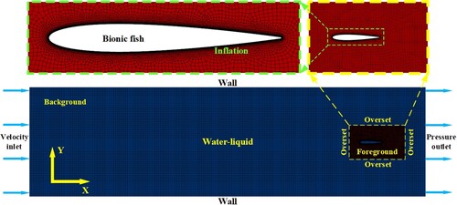
Then the background mesh is divided, and the size of the background area is $18L\times 5L$. The edge cells of the background area are also set to 30 mm, and the surface meshing method of the background area is quadrilaterals. The foreground mesh with fish body boundary layer is unstructured, while the background mesh is structured. After the meshing is completed, the foreground and background mesh overlap, but there is no connection relationship. In order to improve the computational efficiency and accuracy, the number of meshes is controlled under the premise of ensuring the quality of the meshes. The overset mesh contains a total of 119,223 cells and 120,382 nodes. Specifically, the background area contains 100,200 cells and 100,968 nodes. The foreground area contains 19,023 cells and 19,414 nodes. The worst mesh quality is 0.16593, and the average mesh quality is 0.99553. Orthogonal quality is used as the standard. Overset mesh and boundary conditions are shown in Figure 5.

Figure 5. Overset mesh and boundary conditions.

3.3. Mesh independence verification

In order to verify the influence of the mesh size on the numerical simulation results, the mesh is divided into three levels. The size of the background mesh remains the same, and only the foreground and the fish body mesh are changed. The simulation parameters of the three meshes are consistent, $v_{inlet}=0.5$ m/s, h = 0.02 m, $\lambda =0.95$ m, and f = 1.0 Hz. The calculation results show that the difference between the three mesh sizes is not apparent. However, the rough mesh will lead to the distortion of the dynamic mesh during the calculation process, leading to the solution process's instability. The additional meshes will consume many computing resources when the mesh is refined to a certain extent, but it will not significantly improve the numerical simulation results. Therefore, this paper chooses a more reasonable medium mesh. When the self-propelled motion with different parameters is numerically simulated, the consistency of the mesh is maintained, and the influence of the difference of the mesh on the simulation results is eliminated. The three mesh sizes and simulation results are shown in Table 2. We assume that the calculation result of the fine mesh is actual, and the error is 0.

Table 2. Mesh sizes and simulation results.

Mesh size	Fish edge (mm)	Foreground (mm)	Cells	Quality	Results (m/s)	Error
Rough	7	25	113,137	0.99539	−0.280	2.1$\mathrm{\%}$
Medium	5	20	119,223	0.99553	−0.288	0.7$\mathrm{\%}$
Fine	3	15	132,510	0.99586	−0.286	0

3.4. Numerical simulation method

In this study, ANSYS Workbench 2020R2 is used for numerical simulation and prediction. The transient mode and the shear-stress transport (SST) k-ω turbulence model are adopted in this paper. Moreover, the fluid is freshwater, and the foreground and background mesh are set to overset interface. We activate the dynamic mesh option and adopt the diffusion method to smooth the mesh with a diffusion factor of 2. The pressure-velocity coupled solution method is adopted, and the spatial discretization of the pressure is set to second order. Momentum, turbulent kinetic energy, and dissipation rate are all set to second-order upwind. The governing equations are two-dimensional incompressible unsteady Navier-Stokes equations (Ji & Huang, 2017). The mass and momentum conservation expressions are as follows: (12) $\begin{array}{rl}\frac{\mathrm{\partial }u}{\mathrm{\partial }t}+u\frac{\mathrm{\partial }u}{\mathrm{\partial }x}+v\frac{\mathrm{\partial }u}{\mathrm{\partial }y}& =-\frac{1}{\rho }\frac{\mathrm{\partial }p}{\mathrm{\partial }x}+\frac{1}{\rho }\mu {\mathrm{\nabla }}^{2}u\end{array}$(12) (13) $\begin{array}{rl}\frac{\mathrm{\partial }u}{\mathrm{\partial }t}+u\frac{\mathrm{\partial }v}{\mathrm{\partial }x}+v\frac{\mathrm{\partial }v}{\mathrm{\partial }y}& =-\frac{1}{\rho }\frac{\mathrm{\partial }p}{\mathrm{\partial }y}+\frac{1}{\rho }\mu {\mathrm{\nabla }}^{2}v\end{array}$(13) (14) $\begin{array}{rl}{\mathrm{\nabla }}^2& \equiv \frac{{\mathrm{\partial }}^2}{\mathrm{\partial }{x}^2}+\frac{{\mathrm{\partial }}^2}{\mathrm{\partial }{y}^2}\end{array}$(14) (15) $\begin{array}{rl}\frac{\mathrm{\partial }u}{\mathrm{\partial }x}+\frac{\mathrm{\partial }v}{\mathrm{\partial }y}& =0\end{array}$(15) where u represents the velocity component of the x-axis; v represents the velocity component of the y-axis; p represents pressure; ρ represents the density of freshwater; t represents time and ${\mathrm{\nabla }}^2$ 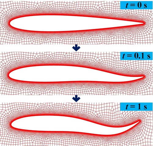represents the Laplacian. The motion of bionic fish is defined by UDF, and the UDF program is embedded in the Fluent in a compiled manner. The motion of the dynamic mesh is shown in Figure 6.

Figure 6. The motion of the dynamic mesh.

4. Numerical simulation results and discussion

Flexible underwater structures with different parameters have different hydrodynamic characteristics (Ghalandari et al., 2019). In order to study the propulsion performance of bionic fish under different parameters, four groups of simulations are performed. The effects of inflow velocity, wave frequency, wavelength, and head fluctuation amplitude are studied. Each group of simulations involves only one parameter change, controlling a single variable. The influence of parameter variation on the velocity of the quasi-steady state, peak acceleration, and displacement is analyzed by simulation results. In addition, the reverse von Karman vortex street (Scaradozzi et al., 2017; Thekkethil et al., 2018; Tytell et al., 2010; Xie et al., 2019) exists in the wake of fish swim, which proves the generation of thrust. Strouhal number ($\mathrm{S}\mathrm{t}$) is a dimensionless number used to characterize the unsteady fluctuation of fish swim wakes. The definition of $\mathrm{S}\mathrm{t}$ in this paper is: (16) $\mathrm{S}\mathrm{t}=\frac{fA}{V}$(16) where f is the wave frequency; A is the tail wave amplitude (Gibouin et al., 2018; Scaradozzi et al., 2017), which is equal to the vertical distance between the highest and lowest point of the tail wave range; V is the upstream velocity.

4.1. Influence of inflow velocity

In order to study the influence of the inflow velocity on the motion state, five simulations are carried out. The inflow velocity ranges from 0.1 m/s to 0.5 m/s, with an interval of 0.1 m/s each time, and other parameters remain the same, f = 1.0 Hz, $\lambda =0.95$ m and h = 0.02 m. Finally, the swimming velocity reaches the critical value and fluctuates slightly up and down, which we define as a quasi-steady state. Gibouin et al. (2018) expressed this conclusion that when a precise balance between thrust and drag is achieved, self-propulsion at a constant speed can be achieved. The simulation results of this paper are shown in Figures 7, 8, and 9.

Figure 7. Velocity contours at different inflow velocities: (a) 0.1 m/s, (b) 0.2 m/s, (c) 0.3 m/s, (d) 0.4 m/s, (e) 0.5 m/s, (f) Reverse von Karman vortex street.

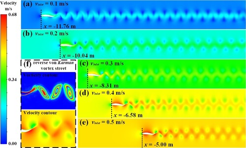
Figure 8. Comparative analysis of inflow velocity: (a) v-t, (b) x-t, (c) a-t, (d) $\mathrm{S}\mathrm{t}$-t.

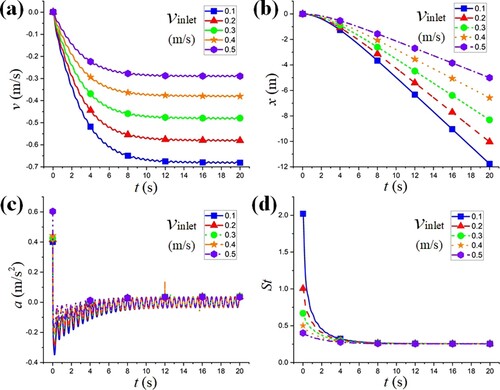
Figure 9. Influence of inflow velocity: (a) v-$v_{inlet}$, (b) x-$v_{inlet}$, (c) a-$v_{inlet}$, (d) $\mathrm{S}\mathrm{t}$-$v_{inlet}$.

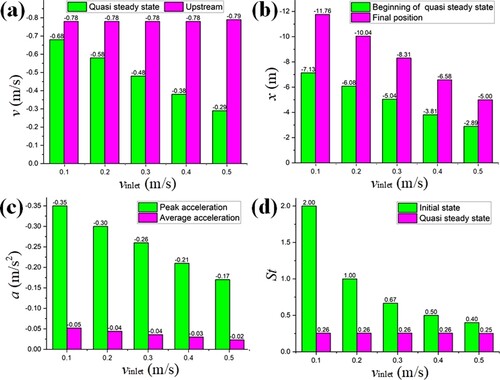
It can be seen from Figures 8 and 9 that when faced with different inflow velocities, the launch state of bionic fish is different, and the swimming velocity of the quasi-steady state is also different. However, the upstream velocity of the quasi-steady state is basically consistent, which is equal to the swimming velocity of the quasi-steady state minus the inflow velocity. The peak acceleration and displacement decrease as the inflow velocity increases. When the five simulations reach the quasi-steady state, the $\mathrm{S}\mathrm{t}$ is basically consistent, and the value is between 0.25 and 0.26. When bionic fish launches at larger inflow velocity, it takes less time to reach the quasi-steady state and corresponds to a smaller displacement. The results show that the inflow velocity has a significant effect on the velocity of the quasi-steady state. When other parameters remain unchanged, the increase of the inflow velocity is equal to the decrease of the velocity of the quasi-steady state.

4.2. Influence of wave frequency

In order to study the influence of wave frequency on propulsion performance, a total of four simulations are carried out at 0.5 Hz, 1.0 Hz, 1.5 Hz, and 2.0 Hz, respectively, of which the simulation at 1.0 Hz has been completed in Section 4.1. The rest of the parameters remain consistent, $v_{inlet}=0.5$ m/s, $\lambda =0.95$ m, and h = 0.02 m. The simulation results are shown in Figures 10, 11, and 12.

Figure 10. Velocity contours and wake vortex structure under different wave frequencies: (a,e) 0.5 Hz, (b,f) 1.0 Hz, (c,g) 1.5 Hz, (d,h) 2.0 Hz.

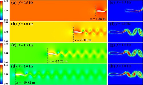
Figure 11. Comparative analysis of wave frequency: (a) v-t, (b) x-t, (c) a-t, (d) $\mathrm{S}\mathrm{t}$-t.

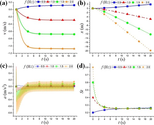
Figure 12. Influence of wave frequency: (a) v-f, (b) x-f, (c) a-f, (d) $\mathrm{S}\mathrm{t}$-f.

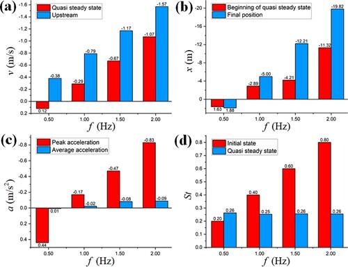
From the simulation results, it can be seen that the thrust generated by the low-frequency wave is insufficient to make bionic fish swim forward but produces a backward velocity under the action of inflow. As the frequency increases, the velocity of the quasi-steady state also increases. In addition, the peak acceleration and displacement increase obviously with the increase of frequency. However, $\mathrm{S}\mathrm{t}$ does not change significantly and remains around 0.25. The quasi-steady state of bionic fish varies considerably when it launches with different wave frequencies. Although the frequency has no significant effect on the time to reach the quasi-steady state, the effect on the displacement is obvious and nonlinear. This means that wave frequency mainly affects velocity and acceleration. In summary, frequency has an important influence on the thrust and explosive power of bionic fish. Reasonable frequency can optimize the velocity of the quasi-steady state and launch response time and further enhance the movement flexibility.

4.3. Influence of wavelength

In order to study the influence of wavelength on propulsion performance, a total of six simulations are carried out at 0.8 m, 0.9 m, 0.95 m, 1.0 m, 1.1 m, and 1.2 m, respectively, of which the 0.95 m simulation has been completed in Section 4.1. The rest of the parameters remain consistent, $v_{inlet}=0.5$ m/s, f = 1.0 Hz and h = 0.02 m. The simulation results are shown in Figures 13, 14, and 15.

Figure 13. Velocity contours at different wavelengths: (a) 0.80 m, (b) 0.90 m, (c) 0.95 m, (d) 1.00 m, (e) 1.10 m, (f) 1.20 m.

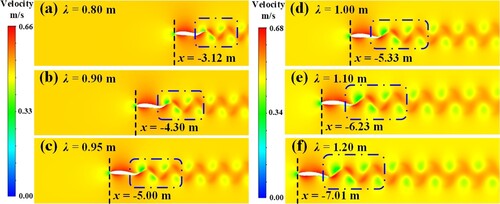
Figure 14. Comparative analysis of wavelength: (a) v-t, (b) x-t, (c) a-t, (d) $\mathrm{S}\mathrm{t}$-t.

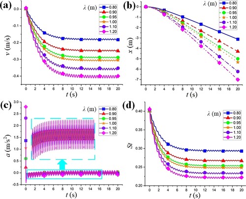
Figure 15. Influence of wavelength: (a) v-λ, (b) x-λ, (c) a-λ, (d) $\mathrm{S}\mathrm{t}$-λ.

The results show that as the wavelength gradually increases from low to high, the swimming velocity of the quasi-steady state increases accordingly, and the peak acceleration overall shows a trend of first decreasing and then increasing. However, $\mathrm{S}\mathrm{t}$ gradually decreases, and the wake vortex becomes more prominent as the wavelength increases. The launch time is similar when the wavelength varies in a small range close to the body length. However, when the wavelength exceeds the body length, the peak acceleration and the displacement to reach the quasi-steady state clearly increase. Obviously, wavelength also has an essential effect on flexibility. When the wavelength is close to the body length, bionic fish has superior movement performance.

4.4. Influence of head fluctuation amplitude

The head fluctuation amplitude is defined as the value of $h\left(x\right)$ when x approaches 0, that is, $h=c_0$, which is consistent with the expression in Section 3.1. In order to study the influence of head fluctuation amplitude on propulsion performance, a total of four simulations are carried out at 0.01 m, 0.02 m, 0.03 m, and 0.04 m, respectively, of which the 0.02 m simulation has been completed in Section 4.1. The rest of the parameters remain consistent, $v_{inlet}=0.5$ m/s, f = 1.0 Hz and $\lambda =0.95$ m. The simulation results are shown in Figures 16, 17, and 18.

Figure 16. Velocity and pressure contours under different head fluctuation amplitudes: (a,e) 0.01 m, (b,f) 0.02 m, (c,g) 0.03 m, (d,h) 0.04 m.

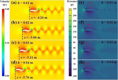
Figure 17. Comparative analysis of head fluctuation amplitude: (a) v-t, (b) x-t, (c) a-t, (d) $\mathrm{S}\mathrm{t}$-t.

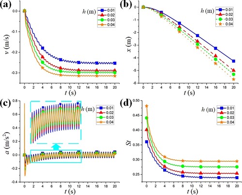
Figure 18. Influence of head fluctuation amplitude: (a) v-h, (b) x-h, (c) a-h, (d) $\mathrm{S}\mathrm{t}$-h.

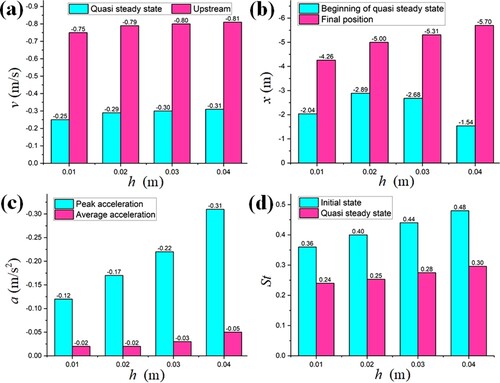
The results show that when the head fluctuation amplitude increases from 0.01 m to 0.02 m, the swimming velocity of the quasi-steady state increases significantly. When the fluctuation amplitude continues to increase, the velocity change is not apparent, but $\mathrm{S}\mathrm{t}$ changes significantly. As the head fluctuation amplitude increases, the launch time to reach the quasi-steady state decreases slightly. Thus, in Figure 18(b), the displacement to reach the quasi-steady state shows an ascending and then descending turn. The velocity increase and launch time decrease indicate that the improved self-propelled motion model has superior motion performance. With the increase of head fluctuation amplitude, the softness of the body is improved, and the width of the wake vortex also improved slightly. It is evident from the pressure contours that the direction of the pressure gradient around the body is slowly changing. Therefore, setting reasonable head fluctuation amplitude is beneficial to improve movement performance.

5. Hydrodynamic prediction and verification

In order to achieve a better propulsion effect, many scholars have adopted novel research methods in recent years. Tytell and Long (2021) coupled the external flow pressure of the robotic fish with the internal neural model. Thandiackal et al. (2021) studied the self-organized wave swimming caused by the peripheral mechanism. Zhong et al. (2021) explored efficient swimming of fish by adjusting tail stiffness. Reasonable wave parameters can produce superior swimming performance. In this paper, CFD simulation data is taken as a training set, and a prediction model is built based on MLP to predict the performance of the optimized parameters. Numerical simulation results show that the predicted results are accurate, and the reliability of the model is high.

5.1. Prediction model

The prediction model based on MLP consists of one input layer, three hidden layers, and one output layer. In addition, each layer contains multiple neurons, and all connections are equipped with weights. Several attempts and error analyses are carried out to determine the number of hidden layers and the number of neurons each layer. The input layer has five variables, and the output layer has four variables. The input layer is only used to obtain input variable information and pass it to the hidden layer without performing any calculations. The input is $x_i$ ($i=0,1,2,3,4,5$), and $x_0$ to $x_4$ represent five characteristic variables. The constant 1 acts as an input bias, represented by $x_5$. Therefore, (17) $x_i^{\mathrm{T}}=[x_0,\dots ,x_i]$(17) Computations are performed in the hidden layer and information is passed to the output layer, and each hidden layer contains a different number of nodes. The first hidden layer contains 128 nodes, the second hidden layer includes 256 nodes, and the third hidden layer involves 256 nodes. The three hidden layers containing 128, 256 and 256 neurons are experimentally validated. The weights of the hidden layer network are $w_{ij}$, $w_{jk}$, and $w_{km}$, respectively. The outputs of the first, second, and third hidden layers are $z_j$, $z_k$, and $z_m$, respectively. The output of each hidden layer is represented as follows: (18) $\begin{array}{rl}{a}_j& =\sum _{i=0}^4{w}_{ji}[x_0,\dots ,x_i]+b_1(j=0,\dots ,127)\end{array}$(18) (19) $\begin{array}{rl}{z}_j& =\tanh \left(a_j\right)\end{array}$(19) (20) $\begin{array}{rl}{a}_k& =\sum _{j=0}^{127}{w}_{kj}[z_0,\dots ,z_j]+b_2(k=0,\dots ,255)\end{array}$(20) (21) $\begin{array}{rl}{z}_k& =\tanh \left(a_k\right)\end{array}$(21) (22) $\begin{array}{rl}{a}_m& =\sum _{k=0}^{255}{w}_{mk}[z_0,\dots ,z_k]+b_3(m=0,\dots ,255)\end{array}$(22) (23) $\begin{array}{rl}{z}_m& =\tanh \left(a_m\right)\end{array}$(23) where $b_1$, $b_2$, $b_3$ respectively represent the bias of each hidden layer; tanh represents the activation function of the hidden layer. The four nodes of the output layer represent the four output characteristic variables. Moreover, the network weight of the output layer is $w_{mo}$, and its transposed matrix is $w_{om}$. Consequently, the output is expressed as: (24) $y_o=\sum _{m=0}^o{w}_{om}{z}_m$(24) Then, $y_o$ is multiplied by $w_{mo}$ to output the data for the characteristic variables. In this paper, the mean square error is used to calculate the loss of $y_o$, and the calculation formula is as follows: (25) $E_r=\frac{1}{2}\sum _{o=0}^{n-1}{(y_o-y_{label})}^2$(25) where n is the number of samples contained in each batch during training, $y_{label}$ is the label corresponding to each sample. The prediction model and the classification of the data set are shown in Figure 19.

Figure 19. MLP prediction model and the classification of the data set.

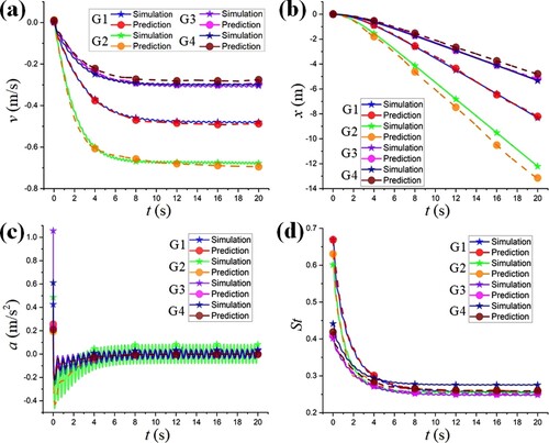
The data of the training model comes from numerical simulation. The simulation calculation sets the time step to 0.005 s and the total time is 20 s. Therefore, the amount of data for each simulation is 4000. The amount of training data provided by each group varies slightly due to the number of simulations. The test set consists of simulation results that are not used as training data or additional simulation results. One simulation is selected from each of the four groups of experiments as the prediction object. The numerical simulation results are compared with the model prediction results, as shown in Figure 20.

Figure 20. Comparison of four groups of simulation results and prediction results: (a) v-t, (b) x-t, (c) a-t, (d) $\mathrm{S}\mathrm{t}$-t.

Meanwhile, a quadratic response surface prediction model is established based on the results of numerical simulation and response surface method (RSM) (J. Liu et al., 2021). Furthermore, the prediction results of the response surface model and the MLP model are compared bidirectionally. The quadratic response surface prediction model is expressed as follows: (26) $\begin{array}{rl}v& =-0.156+1.006v_{inlet}-0.204f+0.15\lambda \\ & +5.125h-0.567f\lambda -2fh-5\lambda h\end{array}$(26) (27) $\begin{array}{rl}x& =-38.853+66.106v_{inlet}+14.679f+36.642\lambda \\ & +313.25h-51.25v_{inlet}\lambda -23.633f\lambda -258fh\end{array}$(27) (28) $\begin{array}{rl}{a}_{max}& =-0.06-0.116v_{inlet}-0.282f+0.217\lambda \\ & +70.427h+0.231v_{inlet}f+16.563v_{inlet}h\\ & -23.125fh-64.167\lambda h\end{array}$(28) (29) $\begin{array}{rl}\mathrm{S}\mathrm{t}& =0.332-0.122\lambda +3.563h-1.75\lambda h\end{array}$(29)

5.2. Parameter optimization and prediction verification

Under the condition that the inflow velocity is 0.5 m/s, the traveling wave parameters of bionic fish are optimized by the multi-objective genetic algorithm (MOGA). It is expected that bionic fish will reach a quasi-steady state swimming velocity of 1.5 m/s to 2 m/s within 30 m under the inflow velocity of 0.5 m/s. The optimization objectives are wave frequency, wavelength and head fluctuation amplitude. A high velocity is achieved within a small displacement by optimizing these parameters. The references show that the optimal swimming performance can be obtained when $\mathrm{S}\mathrm{t}$ is between 0.2 and 0.4 and the tail wave amplitude/body length (A/L) is between 0.1 and 0.3 (H. Liu & Curet, 2018; Saadat et al., 2017). The constraints of multi-objective optimization are as follows: (30) $\{\begin{array}{l}1.5\le v\le 2.0\\ 0\le x\le 30\\ 0.25\le \mathrm{S}\mathrm{t}\le 0.35\\ v_{inlet}=0.5\\ 1.0\le f\le 3.0\\ 0.8\le \lambda \le 1.2\\ 0\le h\le 0.06\end{array}$(30) where v represents the velocity under the quasi-steady state; x represents the displacement at the beginning of the quasi-steady state. Neither v nor x considers the direction of movement. The optimization results are shown in Table 3.

Table 3. Multi-objective optimization results.

Parameters	$v_{inlet}$ (m/s)	f (Hz)	λ (m)	h (m)
Value	0.5	2.7	0.94	0.03

Taking the optimized results as input, CFD, MLP, and RSM are used to predict the hydrodynamic, respectively. The prediction results and the average error are shown in Table 4, where the CFD calculation results are taken as the theoretical truth value, and the error is 0.

Table 4. Comparison of prediction results.

Method	v (m/s)	x (m)	$a_{max}$ (m/s${}^2$)	$\mathrm{S}\mathrm{t}$	Average error
CFD	−1.67	−28.23	−1.79	0.274	0
MLP	−1.68	−28.65	−1.66	0.275	2.4$\mathrm{\%}$
RSM	−1.65	−27.29	−1.68	0.275	2.8$\mathrm{\%}$

It can be seen from the data in Table 4 that the prediction results of the three methods are basically consistent, and the prediction effects of MLP and RSM on velocity and St are better than those on displacement and peak acceleration. The single error of MLP prediction results is within 8$\mathrm{\%}$, and the average error is 2.4$\mathrm{\%}$. The individual error of RSM prediction results is within 7$\mathrm{\%}$, and the average error is 2.8$\mathrm{\%}$. Although the MLP prediction model have no obvious accuracy advantage, the model is efficient in prediction and the process is simple.

In addition, two additional experiments are conducted to further validate the accuracy and generalization ability of the MLP prediction model. Two experiments predict the motion performance of high and low frequency waves at high inflow velocity. The inflow velocity is 1 m/s, and the wave frequency is 2.0 Hz and 3.5 Hz, respectively. The wavelength is 0.95 m and the head fluctuation amplitude is 0.03 m. The results are shown in Tables 5 and 6.

Table 5. Prediction results of low frequency motion (2.0 Hz).

Method	v (m/s)	x (m)	$a_{max}$ (m/s${}^2$)	$\mathrm{S}\mathrm{t}$	Average error
CFD	−0.60	−7.44	−0.83	0.280	0
MLP	−0.61	−8.05	−0.78	0.276	4.3$\mathrm{\%}$
RSM	−0.60	−8.25	−0.68	0.273	7.9$\mathrm{\%}$

Table 6. Prediction results of high frequency motion (3.5 Hz).

Method	v (m/s)	x (m)	$a_{max}$ (m/s${}^2$)	$\mathrm{S}\mathrm{t}$	Average error
CFD	−1.83	−29.11	−2.24	0.278	0
MLP	−1.86	−31.27	−2.06	0.274	4.6$\mathrm{\%}$
RSM	−1.81	−31.52	−1.80	0.273	7.7$\mathrm{\%}$

Although the prediction error of high frequency motion is greater than those of low frequency motion. The average error of two MLP predictions is less than 5$\mathrm{\%}$. The results show that the generalization ability of the MLP prediction model is strong, and the prediction results are accurate and reliable.

6. Conclusions

This paper proposes a hydrodynamic numerical simulation and prediction strategy for the self-propelled motion of bionic fish. This strategy integrates the kinematic model, CFD, MLP, and RSM to achieve efficient and accurate numerical prediction. The effects of inflow velocity, frequency, wavelength, and head fluctuation amplitude on swimming performance are studied by using this strategy. The main conclusions drawn are summarized as follows:

The improved self-propelled model can genuinely simulate the swimming posture of fish. The use of two-dimensional models and overset mesh significantly reduces simulation complexity and achieves high precision while improving simulation efficiency. In addition, UDF is used to drive the movement of bionic fish, which makes the setting of boundary conditions easier and improves the user's manipulation of the calculation process and results.

The self-propelled motion of bionic fish finally reaches the quasi-steady state, the thrust and the resistance are in equilibrium, and the swimming velocity is slightly fluctuating at the critical velocity. Frequency has the most significant effect on velocity of the quasi-steady state of bionic fish, followed by the inflow velocity and wavelength, and the head fluctuation amplitude has the weakest effect. The increase in frequency will improve the thrust and explosive power of bionic fish and reduce the launch time. The wavelength affects the structure of the wake vortex of bionic fish, and the wake vortex gradually increases as the wavelength increases. Moreover, it has superior swimming performance when the wavelength is close to the body length. The increase of head fluctuation amplitude will improve body flexibility and tail wave amplitude, and the direction of the pressure distribution gradient around the body will also change accordingly. In addition, the head fluctuation amplitude has the most obvious effect on $\mathrm{S}\mathrm{t}$ and peak acceleration. When A/L is around 0.2, a superior swimming effect can be obtained.

In summary, the wavelength should be set close to the body length when bionic fish swims, with the head wave amplitude and tail wave amplitude being approximately 3$\mathrm{\%}$ and 20$\mathrm{\%}$ of the body length, respectively. Sufficient power can be obtained when fluctuating at high frequencies within a reasonable range. If all parameters are consistent, quasi-steady state is reached earlier in counter-flow than in down-flow conditions. However, faster quasi-steady state velocity can be achieved in down-flow conditions.

The MLP prediction model constructed in this paper has high accuracy and strong generalization ability, and the average prediction error is within 3$\mathrm{\%}$. The combination of CFD and machine learning can be applied to scientific research and practical engineering. The accuracy of the numerical simulation results is crucial, and the precision of the data affects the accuracy and generalization ability of the prediction model. In order to avoid the accumulation of errors, the accuracy of numerical simulation should be improved as much as possible. However, a simplified fish model is adopted in this paper, and only a two-dimensional numerical simulation is performed. It is a limitation of this paper. In the future, we will extend this strategy to three-dimensional and cluster simulations to obtain more abundant research results. Furthermore, the accuracy and ability of the proposed strategy will further get verification under a much more realistic configuration than the current NACA airfoil.

Acknowledgments

We are very grateful to the experts of the China Graduate Electronics Design Contest for their guidance.

Disclosure statement

The authors declare that they have no known competing financial interests or personal relationships that could have appeared to influence the work reported in this paper.

Correction Statement

This article has been republished with minor changes. These changes do not impact the academic content of the article.

Additional information

Funding

This work was supported by the National Key Research and Development Program of China Grant number 2016YFC0301400 and the National Natural Science Foundation of China Grant number 51379198.

References

- Ariff, M., Salim, S. M., & Cheah, S. C. (2009). Wall y+ approach for dealing with turbulent flow over a surface mounted cube: Part 1-Low Reynolds Number. In Seventh international conference on CFD in the minerals and process industries, CSIRO, Australia, (pp. 1–6).
- Broniszewski, J., & Piechna, J. (2019). A fully coupled analysis of unsteady aerodynamics impact on vehicle dynamics during braking. Engineering Applications of Computational Fluid Mechanics, 13(1), 623–641. https://doi.org/10.1080/19942060.2019.1616326
- Brunton, S. L., Noack, B. R., & Koumoutsakos, P. (2020). Machine learning for fluid mechanics. Annual Review of Fluid Mechanics, 52(1), 477–508. https://doi.org/10.1146/fluid.2020.52.issue-1.
- Chang, X., Zhang, L., & He, X. (2012). Numerical study of the thunniform mode of fish swimming with different Reynolds number and caudal fin shape. Computers & Fluids, 68, 54–70. https://doi.org/10.1016/j.compfluid.2012.08.004
- Colvert, B., Alsalman, M., & Kanso, E. (2018). Classifying vortex wakes using neural networks. Bioinspiration & Biomimetics, 13(2), Article 025003. https://doi.org/10.1088/1748-3190/aaa787
- Cui, Z., Gu, X., Li, K., & Jiang, H. (2017). CFD studies of the effects of waveform on swimming performance of carangiform fish. Applied Sciences, 7(2), 149. https://doi.org/10.3390/app7020149
- Cui, Z., Yang, Z., Shen, L., & Jiang, H. (2018). Complex modal analysis of the movements of swimming fish propelled by body and/or caudal fin. Wave Motion, 78, 83–97. https://doi.org/10.1016/j.wavemoti.2018.01.001
- Dai, Y., Xu, L., Zhu, X., & Ouyang, B. (2021). Application of an unstructured overset method for predicting the gear windage power losses. Engineering Applications of Computational Fluid Mechanics, 15(1), 130–141. https://doi.org/10.1080/19942060.2020.1858166
- Dong, H., Wu, Z., Meng, Y., Tan, M., & Yu, J. (2021). Gliding motion optimization for a biomimetic gliding robotic fish. IEEE/ASME Transactions on Mechatronics. https://doi.org/10.1109/TMECH.2021.3096848
- Gao, L., Qin, H., & Li, P. (2021). Hydrodynamic analysis of fish's traveling wave based on grid deformation technique. International Journal of Offshore and Polar Engineering, 31(2), 178–185. https://doi.org/10.17736/10535381
- Gazzola, M., Hejazialhosseini, B., & Koumoutsakos, P. (2014). Reinforcement learning and wavelet adapted vortex methods for simulations of self-propelled swimmers. SIAM Journal on Scientific Computing, 36(3), B622–B639. https://doi.org/10.1137/130943078
- Ghalandari, M., Bornassi, S., Shamshirband, S., Mosavi, A., & Chau, K. W. (2019). Investigation of submerged structures' flexibility on sloshing frequency using a boundary element method and finite element analysis. Engineering Applications of Computational Fluid Mechanics, 13(1), 519–528. https://doi.org/10.1080/19942060.2019.1619197
- Gibouin, F., Raufaste, C., Bouret, Y., & Argentina, M. (2018). Study of the thrust–drag balance with a swimming robotic fish. Physics of Fluids, 30(9), Article 091901. https://doi.org/10.1063/1.5043137
- Guang, R., Chao, W., & Fei, W. (2014). A traveling wave fitting method for robotic fish with a multi-joint caudal fin. In The 26th Chinese Control and Decision Conference (2014 CCDC) (pp. 3311-3315). IEEE.
- Han, P., Lauder, G. V., & Dong, H. (2020). Hydrodynamics of median-fin interactions in fish-like locomotion: Effects of fin shape and movement. Physics of Fluids, 32(1). https://doi.org/10.1063/1.5129274
- Huang, X., Cheng, C., & Zhang, X b. (2021). Machine learning and numerical investigation on drag reduction of underwater serial multi-projectiles. Defence Technology, 229–237. https://doi.org/10.1016/j.dt.2020.12.002
- Ji, F., & Huang, D. (2017). Effects of Reynolds number on energy extraction performance of a two dimensional undulatory flexible body. Ocean Engineering, 142, 185–193. https://doi.org/10.1016/j.oceaneng.2017.07.005
- Kandula, M., Nallasamy, R., Schallhorn, P., & Duncil, L. (2008). An application of overset grids to payload/fairing three-dimensional internal flow CFD analysis. Engineering Applications of Computational Fluid Mechanics, 2(1), 119–129. https://doi.org/10.1080/19942060.2008.11015215
- Khalid, M. S. U., Akhtar, I., Imtiaz, H., Dong, H., & Wu, B. (2018). On the hydrodynamics and nonlinear interaction between fish in tandem configuration. Ocean Engineering, 157, 108–120. https://doi.org/10.1016/j.oceaneng.2018.03.049
- Kochkov, D., Smith, J. A., Alieva, A., Wang, Q., Brenner, M. P., & Hoyer, S. (2021). Machine learning–accelerated computational fluid dynamics. Proceedings of the National Academy of Sciences, 118(21), 1–8. https://doi.org/10.1073/pnas.2101784118.
- Li, N., Zhang, D. Q., Liu, H. T., & Li, T. J. (2021). Optimal design and strength reliability analysis of pressure shell with grid sandwich structure. Ocean Engineering, 223, Article 108657. https://doi.org/10.1016/j.oceaneng.2021.108657
- Li, R., Xiao, Q., Liu, Y., Li, L., & Liu, H. (2020). Computational investigation on a self-propelled pufferfish driven by multiple fins. Ocean Engineering, 197. https://doi.org/10.1016/j.oceaneng.2019.106908
- Li, S., Yang, W., Xu, L., & Li, C. (2019). An environmental perception framework for robotic fish formation based on machine learning methods. Applied Sciences, 9(17), 3573. https://doi.org/10.3390/app9173573
- Lighthill, M. (1960). Note on the swimming of slender fish. Journal of Fluid Mechanics, 9(2), 305–317. https://doi.org/10.1017/S0022112060001110
- Liu, G., Ren, Y., Dong, H., Akanyeti, O., Liao, J. C., & Lauder, G. V. (2017). Computational analysis of vortex dynamics and performance enhancement due to body–fin and fin–fin interactions in fish-like locomotion. Journal of Fluid Mechanics, 829, 65–88. https://doi.org/10.1017/jfm.2017.533
- Liu, H., & Curet, O. (2018). Swimming performance of a bio-inspired robotic vessel with undulating fin propulsion. Bioinspiration & Biomimetics, 13(5), Article 056006. https://doi.org/10.1088/1748-3190/aacd26
- Liu, J., He, B., Yan, T., Yu, F., & Shen, Y. (2021). Study on carbon fiber composite hull for AUV based on response surface model and experiments. Ocean Engineering, 239. https://doi.org/10.1016/j.oceaneng.2021.109850
- Liu, J., & Hu, H. (2010). Biological inspiration: From carangiform fish to multi-joint robotic fish. Journal of Bionic Engineering, 7(1), 35–48. https://doi.org/10.1016/S1672-6529(09)60184-0
- Ma, Q., Ding, L., & Huang, D. (2021). A study on the influence of schooling patterns on the energy harvest of double undulatory airfoils. Renewable Energy, 174, 674–687. https://doi.org/10.1016/j.renene.2021.04.053
- Ming, T., Jin, B., Song, J., Luo, H., Du, R., & Ding, Y. (2019). 3D computational models explain muscle activation patterns and energetic functions of internal structures in fish swimming. PLoS Computational Biology, 15(9), Article e1006883. https://doi.org/10.1371/journal.pcbi.1006883
- Novati, G., Verma, S., Alexeev, D., Rossinelli, D., Van Rees, W. M., & Koumoutsakos, P. (2017). Synchronisation through learning for two self-propelled swimmers. Bioinspiration & Biomimetics, 12(3), Article 036001. https://doi.org/10.1088/1748-3190/aa6311
- Saadat, M., Fish, F. E., Domel, A., Di Santo, V., Lauder, G., & Haj-Hariri, H. (2017). On the rules for aquatic locomotion. Physical Review Fluids, 2(8), Article 083102. https://doi.org/10.1103/PhysRevFluids.2.083102
- Salih, S. Q., Aldlemy, M. S., Rasani, M. R., Ariffin, A., Ya, T. M. Y. S. T., Al-Ansari, N., Yaseen, Z. M., & Chau, K. W. (2019). Thin and sharp edges bodies-fluid interaction simulation using cut-cell immersed boundary method. Engineering Applications of Computational Fluid Mechanics, 13(1), 860–877. https://doi.org/10.1080/19942060.2019.1652209
- Scaradozzi, D., Palmieri, G., Costa, D., & Pinelli, A. (2017). BCF swimming locomotion for autonomous underwater robots: A review and a novel solution to improve control and efficiency. Ocean Engineering, 130, 437–453. https://doi.org/10.1016/j.oceaneng.2016.11.055
- Shen, X., Zheng, Y., & Zhang, R. (2020). A hybrid forecasting model for the velocity of hybrid robotic fish based on back-propagation neural network with genetic algorithm optimization. IEEE Access, 8, 111731–111741. https://doi.org/10.1109/Access.6287639
- Shi, Y., Xu, Y., Zong, K., & Xu, G. (2017). An investigation of coupling ship/rotor flowfield using steady and unsteady rotor methods. Engineering Applications of Computational Fluid Mechanics, 11(1), 417–434. https://doi.org/10.1080/19942060.2017.1308272
- Su, D., Xu, G., Huang, S., & Shi, Y. (2019). Numerical investigation of rotor loads of a shipborne coaxial-rotor helicopter during a vertical landing based on moving overset mesh method. Engineering Applications of Computational Fluid Mechanics, 13(1), 309–326. https://doi.org/10.1080/19942060.2019.1585390
- Sun, X., Ji, F., Zhong, S., & Huang, D. (2020). Numerical study of an undulatory airfoil with different leading edge shape in power-extraction regime and propulsive regime. Renewable Energy, 146, 986–996. https://doi.org/10.1016/j.renene.2019.06.106
- Tanha, M., & Feeny, B. F. (2019). Evaluation of traveling wave models for carangiform swimming based on complex modes. In Topics in modal analysis & testing (Vol. 9, pp. 335–341). Springer.
- Thandiackal, R., Melo, K., Paez, L., Herault, J., Kano, T., Akiyama, K., Dimitri Ryczko, F. B., Ishiguro, A., & A. J. Ijspeert (2021). Emergence of robust self-organized undulatory swimming based on local hydrodynamic force sensing. Science Robotics, 6(57), Article eabf6354. https://doi.org/10.1126/scirobotics.abf6354
- Thekkethil, N., Sharma, A., & Agrawal, A. (2018). Unified hydrodynamics study for various types of fishes-like undulating rigid hydrofoil in a free stream flow. Physics of Fluids, 30(7), Article 077107. https://doi.org/10.1063/1.5041358
- Tian, F. B. (2020). Hydrodynamic effects of mucus on swimming performance of an undulatory foil by using the DSD/SST method. Computational Mechanics, 65(3), 751–761. https://doi.org/10.1007/s00466-019-01792-2
- Tytell, E. D., Hsu, C. Y., Williams, T. L., Cohen, A. H., & Fauci, L. J. (2010). Interactions between internal forces, body stiffness, and fluid environment in a neuromechanical model of lamprey swimming. Proceedings of the National Academy of Sciences, 107(46), 19832–19837. https://doi.org/10.1073/pnas.1011564107
- Tytell, E. D., & Long Jr., J. H. (2021). Biorobotic insights into neuromechanical coordination of undulatory swimming. Science Robotics, 6(57), Article eabk0620. https://doi.org/10.1126/scirobotics.abk0620
- Videler, J., & Hess, F. (1984). Fast continuous swimming of two pelagic predators, saithe (Pollachius virens) and mackerel (Scomber scombrus): A kinematic analysis. Journal of Experimental Biology, 109(1), 209–228. https://doi.org/10.1242/jeb.109.1.209
- Wang, L., & Wu, C. (2010). An adaptive version of ghost-cell immersed boundary method for incompressible flows with complex stationary and moving boundaries. Science China Physics, Mechanics and Astronomy, 53(5), 923–932. https://doi.org/10.1007/s11433-010-0185-z
- Xie, F., Li, Z., Ding, Y., Zhong, Y., & Du, R. (2019). An experimental study on the fish body flapping patterns by using a biomimetic robot fish. IEEE Robotics and Automation Letters, 5(1), 64–71. https://doi.org/10.1109/LSP.2016.
- Xu, D., Lv, Z., Liu, J., & Wang, J. (2017). A novel artificial lateral line sensing system of robotic fish based on BP neural network. In 2017 12th IEEE conference on industrial electronics and applications (ICIEA) (pp. 1386–1390).
- Yan, L., Chang, X., Tian, R., Wang, N., Zhang, L., & Liu, W. (2020). A numerical simulation method for bionic fish self-propelled swimming under control based on deep reinforcement learning. Proceedings of the Institution of Mechanical Engineers, Part C: Journal of Mechanical Engineering Science, 234(17), 3397–3415. https://doi.org/10.1177/0954406220915216
- Yao, Z., Zhang, N., Chen, X., Zhang, C., Xia, H., & Li, X. (2020). The effect of moving train on the aerodynamic performances of train-bridge system with a crosswind. Engineering Applications of Computational Fluid Mechanics, 14(1), 222–235. https://doi.org/10.1080/19942060.2019.1704886
- Yong-hua, Z., Shi-wu, Z., Jie, Y., & Low, K.. (2007). Morphologic optimal design of bionic undulating fin based on computational fluid dynamics. In 2007 International conference on mechatronics and automation (pp. 491496). IEEE.
- Zhang, D., Pan, G., Chao, L., & Zhang, Y. (2018). Effects of Reynolds number and thickness on an undulatory self-propelled foil. Physics of Fluids, 30(7). https://doi.org/10.1063/1.5034439
- Zhao, Z., & Dou, L. (2019a). Computational research on a combined undulating-motion pattern considering undulations of both the ribbon fin and fish body. Ocean Engineering, 183, 1–10. https://doi.org/10.1016/j.oceaneng.2019.04.094
- Zhao, Z., & Dou, L. (2019b). Effects of the structural relationships between the fish body and caudal fin on the propulsive performance of fish. Ocean Engineering, 186. https://doi.org/10.1016/j.oceaneng.2019.106117
- Zhong, Q., Zhu, J., Fish, F., Kerr, S., Downs, A., Bart-Smith, H., & Quinn, D. (2021). Tunable stiffness enables fast and efficient swimming in fish-like robots. Science Robotics, 6(57), Article eabe4088. https://doi.org/10.1126/scirobotics.abe4088
- Zhou, C., Nahavandi, S., Gu, N., Cao, Z., Wang, S., & Tan, M. (2008). Analysis and implementation of swimming backward for biomimetic carangiform robot fish. IFAC Proceedings Volumes, 41(2), 3082–3086. https://doi.org/10.3182/20080706-5-KR-1001.00523
- Zhou, H., Hu, T., Low, K. H., Shen, L., Ma, Z., Wang, G., & Xu, H. (2015). Bio-inspired flow sensing and prediction for fish-like undulating locomotion: A CFD-aided approach. Journal of Bionic Engineering, 12(3), 406–417. https://doi.org/10.1016/S1672-6529(14)60132-3
- Zhou, H., Hu, T., Xie, H., Zhang, D., & Shen, L. (2010). Computational hydrodynamics and statistical modeling on biologically inspired undulating robotic fins: A two-dimensional study. Journal of Bionic Engineering, 7(1), 66–76. https://doi.org/10.1016/S1672-6529(09)60192-X