Swirl flow in annular geometry with varying cross-section

Abstract

Swirling gas flow is an important topic of research that helps in the design of rockets, atomizers,and gas turbine combustors. In the present work, swirl flow inside annular geometries with constant and varying cross-sectional areas are examined using computational fluid dynamics (CFD). Effects of changing the flow and geometric parameters on the swirl behaviour were studied. Reynolds number was found to increase the swirl number in straight and diverging cross-sectional geometries while no significant effect of Reynolds number was observed in converging cross-sectional geometry. Radius ratio, defined as the ratio of the inner to the outer radius of the annular geometry, was found to have a significant effect on the swirl number. Decreasing the radius ratio, in straight and diverging annular geometry decreases the swirl number, however, an opposite trend was observed in the case of converging annular geometry due to significant increase in axial velocity as a result of reduced cross-sectional area. Increasing the swirler vane angle increased the swirl number. At higher vane angles of 60° and 70°, a recirculation zone is developed near the exit of the swirler. Using small cone angles was found to lower the swirl decay rate in converging and diverging nozzles.

KEYWORDS:

• Swirl
• swirl flow
• annulus
• converging annulus
• diverging annulus
• varying cross-sectional annuli

Introduction

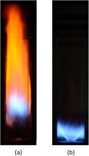
Swirl flows apart from having axial velocity also have a spiraling motion or a tangential velocity (azimuthal direction) component, which is generally imparted by the use of vanes or tangential entry of the flow in a chamber (Gupta et al., 1984). Swirl flows are used in many non-reacting applications such as vortex amplifiers, cyclone separators (Carlos Berrio et al., 2018; Erdal & Shirazi, 2004; Pang et al., 2022), heat exchangers (Sheikholeslami et al., 2015), pumps (Guillaume & Judge, 2004; Zhao et al., 2021), bubble generators (Alam et al., 2018), for cooling purposes using nano particles (Granados-Ortiz et al., 2021) etc. and reacting applications such as solid-propellant rocket motors (Norton et al., 1969), liquid rocket engines (Chiaverhi et al., 2002) ramjets (Chang et al., 1989), spray nozzles (Biswas & Som, 1986), atomizers (Abo-Elfadl & Abd El-Sabor Mohamed, 2018; Taylor, 1950) and gas turbine combustors (Carlanescu et al., 2018; Koh et al., 2001). Swirl flows are widely used and are vital in combustion systems such as rocket engines and gas turbines (Sui et al., 2021) because of their advantages in the stabilization of high-intensity combustion. Swirl flows are known to enhance the mixing of fuel and oxidizer near the exit of nozzles and on the boundaries of recirculation zones. The formation of toroidal re-circulation zones in swirling flows enhances the stability of combustion as they are a well-mixed zone of combustion products and also act as a storage for heat and chemically active species (Gupta et al., 1984). Swirl flows can also minimize flame impingement, i.e. flame impinging on regions not designed to handle high temperature, reducing the maintenance and improving the longevity of the burner (Syred & Beér, 1974). Figure 1 shows the difference between non-swirl and swirl stabilized premixed flow in a burner. It can be seen that the non-swirl flame is longer in length and is detached from the base of the burner while producing a red plume, indicative of unburnt hydrocarbons. On the other hand, the flame stabilized by swirl flow is firmly attached to the base of the combustor without having red regions in the flame indicating no unburnt hydrocarbons are produced.

Figure 1. Comparison of flame shapes (a) non-swirl flow (b) swirl flow.

Swirl flows are characterized by a non-dimensional number called Swirl number, which is defined as the ratio of the axial flux of swirl momentum to the axial flux of axial momentum times the radius (Gupta et al., 1984), (1) $S=\frac{G_{\theta }}{R{G}_x}=\frac{\left({\int }_0^R\overline{u}\overline{w}{r}^{2}dr\right)}{R{\int }_0^R\overline{u^2}rdr}$(1) $G_{\theta }$ is the axial flux of swirl momentum, $G_x$ is the axial flux of the axial momentum, R is the radius (Gupta et al., 1984), $\overline{u}$ and $\overline{w}$ 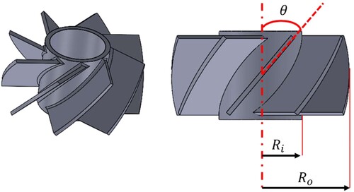are the axial and tangential velocity component of the flow. When using a swirl generator with vanes, such as that shown in Figure 2, the swirl number can also be calculated as (Gupta et al., 1984): (2) $S=\frac{2}{3}\left[\frac{\left(1-{\left(\frac{R_i}{R_o}\right)}^3\right)}{1-{\left(\frac{R_i}{R_o}\right)}^2}\right]\tan \left(\theta \right)$(2) where $R_i$ is the radius of the inner hub of the swirl generator, $R_o$ is the radius of the outer hub and $\theta$ is the inclination of the vanes with respect to the center axis of the swirler. Several other definitions for swirl numbers used in the literature have been reported by Vaziri and Shahsavand (2015).

Figure 2. Flat-vane axial swirl generators.

Swirl flows in circular geometries of varying cross-sectional area has been studied by many researchers for different applications. Algifri et al. (1988) studied the eddy viscosity in decaying swirl flow in a pipe. They developed a correlation to determine the eddy viscosity as a function of Reynolds number and swirl number. Lineberry (1968) experimentally studied swirling airflow in a converging nozzle. He found that the converging nozzle tended to increase the magnitude of the axial velocity component. Leclaire et al. (2005) experimentally studied the effect of contraction on a rotating flow. They found that depending upon the upstream flow, the flow inside the nozzle can have recirculation zones at the center. Namet-Allah and Birk (2014) carried out a numerical and experimental study on swirling flow in a short annular to round nozzle. They found the flow uniformity at the nozzle exit to decrease with an increase in swirl strength. The size of the recirculation zone downstream of the flow was found to increase with an increase in swirl number. Islam et al. (2020, Khan et al., 2020) numerically examined a swirl nozzle with different geometries that use an aerodynamic swirl. Different shapes; a straight, tapered cone, and a nozzle with a 5th-degree polynomial curve were examined along with a number of tangential inlets. The study was carried out using Menter’s Shear Stress Transport (SST) k-ω turbulence model. They found the axial and tangential velocity to be heavily dependent on the number of tangential inlets. High axial and tangential velocities were reported for shape with 5th degree polynomial shaped converging nozzle.

Cloos and Pelz (2019) experimentally studied the swirl development at the inlet of a coaxial rotating diffuser. They found that the evolution of the swirl depended upon the Reynolds number, axial coordinate and the apex angle. Degenève et al. (2019) experimentally studied the effect of diverging angle. They found the diverging nozzle, on the swirl number and shape of a premixed flame. They observed that with increasing cup angle the flame became shorter and almost becomes flat at a cup angle of 45°. Higher axial and tangential velocities were observed at lower values of the cup angle. As a result, the swirl number inside the combustor was found to decrease with an increase in the cup angle of the nozzle before the combustor. Agarwal and Mthembu (Agarwal & Mthembu, 2020) studied conical diffusers using swirl angles of 10°–30°. They used the RNG k-ε model for modeling the turbulence using Ansys Fluent. They observed maximum pressure drops with 20° diffuser cone angles. Clayton and Morsi (Clayton & Morsi, 1984) experimentally investigated the decay of swirl in a straight annulus with different vane angles and Reynolds numbers. They found that the rate of swirl decay increases with an increase in radius ratio and inlet swirl but decreases with an increase in Reynolds number. Yan et al. (2020) studied the swirl generation using a multi-lobed swirl generator and also investigated the rate of swirl decay by modeling the turbulence using Reynolds Stress Model (RSM). They found the swirl number to first increase up till lobe number 4 and then decrease with increase in number of lobes. Choi et al. (2018) modeled the swirl decay rate of turbulent swirling flows in annular swirl injectors with straight and converging cross-sectional areas. They developed a 1-D ordinary differential equation (ODE) to predict the swirl number inside annular straight and converging geometries. The ODE was validated using results from Large Eddy Simulations (LES) which are computationally expensive. They studied the effect of Reynolds number and vane angles on Swirl number in straight and converging annular geometries. Furthermore, they used the developed ODE to predict the critical swirl number that leads to the generation of a central-toroidal recirculation zone inside a gas turbine combustor.

Annular geometries are often used in the design of burners and are prominently used in stratified flame burners (Fiorina et al., 2015; Franke et al., 2017; Sweeney et al., 2012) to introduce inhomogeneity in the reacting mixtures, which enhances the flame stability and increases its operability regime. This enables such burners to operate at ultra-lean conditions to prevent NOx formation (Masri, 2015). Stratified burners contain a multitude of annuli to enable flame stratification. Each of the annuli can be designed to have a constant or varying cross-sectional area. It is imperative to understand the behavior of swirling flow in variable annular geometries to inform and aid the decision-making process when designing annular burners. Most of the previous studies related to swirling flow in variable cross-section geometries deal with non-annular geometries. A few studies have investigated swirling flow in straight annulus and converging annulus, but not on diverging annulus. Furthermore, it is imperative to understand and contrast the behavior of swirling flows in straight, converging and diverging annulus. Thus, there is a gap in the literature regarding the behavior of swirling flows in annular geometries with varying cross-sectional areas, specially. In the present work turbulent swirl flow in a straight, converging and diverging annular geometry is studied using the CFD technique. A parametric study on the effects of Reynolds number, radius ratio, cone angle and swirler vane angle was carried out to determine the important factors affecting the swirl behavior inside different annular geometries.

Methodology

The numerical modeling of the flow through the annular geometries was carried out using Ansys Fluent 2020 R² commercial code. The flow is assumed to be isothermal, therefore, only the continuity and momentum equations are solved. Furthermore, the continuity and momentum equations are solved using the steady-state assumption. The steady-state continuity equation is written as: (3) $\frac{\mathrm{\partial }}{\mathrm{\partial }{x}_j}\left(\rho u_j\right)=0$(3)

The steady-state momentum equation is written as: (4) $\frac{\mathrm{\partial }\left(\rho u_i{u}_j\right)}{\mathrm{\partial }{x}_j}=-\frac{\mathrm{\partial }P}{\mathrm{\partial }{x}_i}+\frac{\mathrm{\partial }\left({\tau }_{ij}\right)}{\mathrm{\partial }{x}_j}$(4) where ${\tau }_{ij}$ is the viscous stress tensor given by: (5) ${\tau }_{ij}=\mu \left[\left(\frac{\mathrm{\partial }{u}_i}{\mathrm{\partial }{x}_j}+\frac{\mathrm{\partial }{u}_j}{\mathrm{\partial }{x}_i}\right)-\frac{2}{3}\frac{\mathrm{\partial }{u}_k}{\mathrm{\partial }{x}_k}{\delta }_{ij}\right]$(5)

Here, ${\delta }_{ij}=1\text{if}i=j$, ${\delta }_{ij}=0\text{if}i\ne j$

where $\rho$ is the density, u is the velocity component in a particular direction, $P$ is the pressure and $\mu$ is the viscosity.

Turbulent flows have fluctuating velocity fields. These fluctuations also affect the transport properties like the momentum, energy, and species and cause them to fluctuate as well. Turbulent flows are computationally expensive to simulate in comparison to laminar flows. Direct Numerical Solution (DNS) is the most advanced technique to simulate a turbulent flow. But it requires the distance between the grid spacing to be smaller than that of the Kolmogorov scale. Therefore, even with ever so advancing computation power, the DNS technique is time-consuming, especially for swirling flows (Dinesh et al., 2015; Ranga Dinesh et al., 2014) and can take up to million CPU hours. An alternate to DNS is the use of the Large Eddy Simulation (LES) technique. LES models are used to understand the time evolution of turbulent flow structures at very fine scales. It splits the turbulent length scales so that large scales are resolved directly as in DNS, while the smaller scales are filtered and modeled. This decreases the mesh resolution required; however, the computational time is still high often requiring days for the solution of a single case (Herff et al., 2021), limiting the number of parameters that can be studied using the LES model. The classical approach to modeling turbulent flows is based on single-point averages of the Navier-stokes equations. The flow governing equations are time-averaged to give a modified set of equations called the Reynolds Averaged Navier-Stokes (RANS) equation.

The time-averaged, steady-state momentum equation is written as (6) $\frac{\mathrm{\partial }}{\mathrm{\partial }{x}_j}\left(\rho u_i{u}_j\right)=-\frac{\mathrm{\partial }p}{\mathrm{\partial }{x}_i}+\frac{\mathrm{\partial }{\tau }_{ij}}{\mathrm{\partial }{x}_j}+\frac{\mathrm{\partial }}{\mathrm{\partial }{x}_j}\left(-\rho \overline{u_i^{\mathrm{\prime }}{u}_j^{\mathrm{\prime }}}\right)$(6)

Equation (6) is called the Reynolds averaged Navier-Stokes equation. However, additional terms representing the effects of turbulence called the Reynolds stresses, $-\rho \overline{u_i^{\mathrm{\prime }}{u}_j^{\mathrm{\prime }}}$ now appear. These terms need to be modeled in order to provide closure for the momentum equation. Several turbulence models are available in the literature to model the turbulent flow. However, not all turbulence models can be used for any given case. The standard two-equation k-ε model has been used by many to model swirling flows with good predictions (Marzouk & David Huckaby, 2010). Others have used the RNG k-ε model (Aliyu et al., 2016; Habib et al., 2012; Shakeel et al., 2018), Realizable k-ε model (Van Maele et al., 2003), SST (Shear Stress Transport) k-ω model (Lee et al., 2021) and Reynolds stress model (RSM) (Hogg & Leschziner, 1989; Jawarneh & Vatistas, 2006; Yang et al., 2003) with varying degree of success to model swirling flows. Initial runs were carried out for the assessment of the best RANS model for the present study.

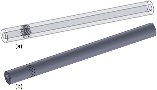
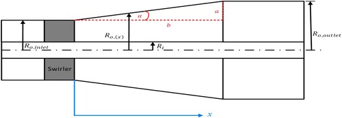
A 3-D geometry was created for the cases under study. Figure 3(a) shows the 3-D model for one of the annular geometries while Figure 3(b) shows the fluid domain used for the simulation. Velocity inlet boundary condition was used at the inlet. The fluid used for the simulation was air at a constant temperature of 25 °C. An outflow condition was used at the outlet (Neumann boundary condition).

Figure 3. A 3-D model for annular pipe geometry with swirler.

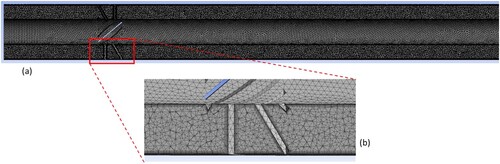
Tetrahedral elements were used to create a mesh for the fluid domain due to the complexity introduced by the blades of the swirler. Inflation layers were used near the walls to capture the boundary layer near the walls. The inflation region consisted of 15 layers such that the wall y⁺ throughout the domain was in the range of 1–3.5. Figure 4(a) shows the mesh used for the study, while Figure 4(b) shows the inflation layers used near the walls.

Figure 4. (a) Mesh used for the study (b) Shows inflation layer used near the walls.

A mesh independence study was carried out to determine the appropriate element size that can be used without increasing the computational effort to prohibitive levels. Figure 5 shows the variation of swirl numbers along the axis of the fluid domain for different mesh sizes (different number of elements, ranging from 59,000 to 4.5 million elements). Table 1 shows the mesh size and the corresponding element size used in the creation of the mesh along with the percentage difference of swirl number (at the exit) from the previous mesh size. The mesh with 2.5 million elements is able to give similar results to that of 3.3 and 4.5 million elements. Therefore, in all further studies, element size of 10⁻³ meters has been used. A large number of mesh elements are required due to the complexity of the geometry which includes the vanes of the swirler.

Figure 5. Mesh independence study.

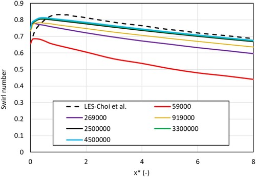
Table 1. Mesh size and corresponding element size.

Number of elements	Element size	Percentage difference in swirl number at exit from previous mesh size
59000	5 × 10^−3 m
269000	2.5 × 10^−3 m	39.18%
919000	1.5 × 10^−3 m	7.69%
2500000	1 × 10^−3 m	5.81%
3300000	9 × 10^−4 m	0.79%
4500000	8 × 10^−4 m	0.42%

Table 2. Values of coefficients used in Equation (12) along with the value of R² for the correlation and the average error.

	For converging section	For straight annular section after the converging section
$a_0$	0.5570	−3.664
$a_1$	0.0368	−0.0073
$a_2$	−0.4668	−0.5613
$a_3$	−0.3089	0.657
$a_4$	−0.2460	18.94
$a_5$	−0.2072	−0.19
$a_6$	0	−21.823
$a_7$	−0.0909	−0.0726
$a_8$	−0.1333	−0.0500
$a_9$	−0.0399	0.0648
$a_{10}$	−0.2528	0.0621
$a_{11}$	0.1251	0
$a_{12}$	−0.9882	−1.046
R^2	0.98	0.98
Average error	4.8%	4.3%

Table 3. Values of coefficients used in Equation (14) along with the value of R² for the correlation and the average error.

$a_1$	0.1960
$a_2$	−0.9823
$a_3$	−0.0203
$a_4$	−1.4303
$a_5$	0.3470
$a_6$	0.0706
$a_7$	0.0671
$a_8$	0.3019
$a_9$	0.1242
$a_{10}$	0.0311
R^2	0.98
Average error	5.9%

Validation

In order to validate the numerical model, the results from the Fluent model were validated with that presented by Choi et al. (2018) using the LES model. The validation is carried out for two of the cases, straight annular geometry and converging annular geometry. Additional validation exercise was carried out with the experimental data for straight annulus, from the work of Clayton and Morsi (1984).

Straight annulus

Figure 6 shows the non-dimensionalized tangential velocity vs the non-dimensionalized length of the straight annulus with a Reynolds number (Re) of 12000. The angle (θ) of the flat vanes was 45° and the $R_i/R_{o,inlet}$ ratio $\left(\gamma \right)$ was 7/14. The non dimensionalization of the tangential velocity was carried out by diving it with the axial velocity at the inlet of the annulus, while the length was non-dimensionalized by diving it with the outer radius. Figure 7 shows the variation of swirl number along the straight annulus. The swirl number at any point is calculated using the following equation (Choi et al., 2018): (7) $S_w\left(x\right)=\frac{2}{3}\left(\frac{1-{\gamma }^3}{1-{\gamma }^2}\right)\tan \left(\frac{V_{\theta }\left(x\right)}{V_{ax}\left(x\right)}\right)$(7) where $\gamma =R_i/R_{o,inlet}$, $V_{\theta }\left(x\right)$ is the tangential velocity component at any position $x$ and $V_{ax}\left(x\right)$ is the axial velocity component.

Figure 6. Validation of non-dimensionalized tangential velocity along the straight annulus with results from Choi et al. (2018) (Re = 12000, θ = 45°, γ = 7/14).

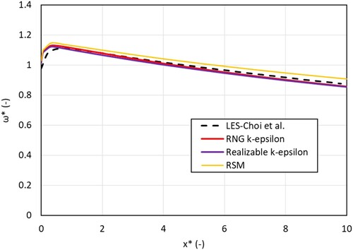
Figure 7. Validation of Swirl number along the straight annulus with results from Choi et al. (2018) (Re = 12000, θ = 45°, γ = 7/14).

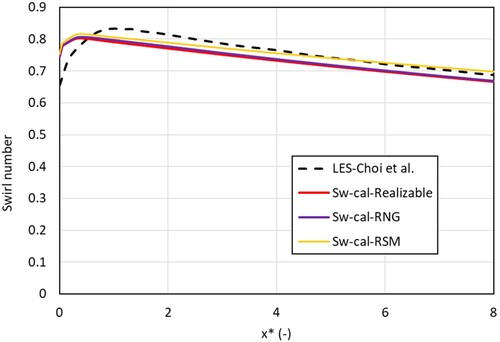
The RNG k-ε, realizable k-ε and Reynolds Stress Model (RSM) were used to model the flow. The RNG k-ε and realizable k-ε models are two-equation models while the RSM model uses 7 equations to model the turbulence. SIMPLE algorithm was used for pressure-velocity coupling. It can be seen from Figures 6 and 7 that all three models are able to predict the flow tangential velocity and the swirl number with reasonable accuracy, however, immediately after the swirler in the developing region of the flow, the position of the peak swirl number has a small discrepancy. Much better prediction is obtained with the three RANS models in the developed flow region. RSM slightly overpredicts the tangential velocity, while RNG k-ε and the Realizable k-ε model underpredict the tangential velocity. A maximum deviation of 2.1%, 2.6% and 3.66% from the LES results were observed for non-dimensionalized tangential velocity when using RNG k-ε, Realizable k-ε and RSM models, respectively. For the RNG k-ε, Realizable k-ε models, the Menter-Lechner wall functions were used due to the robustness and better accuracy (Menter, 1994). While, enhanced wall treatment function was used for the RSM. All three models gave a maximum deviation of about 15% in swirl number prediction immediately after the swirler, however, in the developed region the maximum deviation was 3.1%, 3.3% and 2.4% for RNG k-ε, Realizable k-ε and RSM models, respectively. The solutions were assumed to be converged when the residuals for the continuity and momentum equations reached a value below 10⁻⁵. For a fully converged solution, on a 2.3 GHz, 16 core Haswell processor with 128 GB of DDR4 memory the RNG k-ε and Realizable k- ε models required 30–40 core hours to solve the problem while the RSM model required 130–150 core hours. The increased complexity of the 7-equation RSM model necessitated the use of significantly lower under relaxation factors (between 0.2 and 0.3) to provide a stable solution. This is due to the need to model pressure strain in the RSM model which can pose a significant challenge and lead to numerical stiffness and stability issues (Elkhoury, 2017). All three models gave good predictions in the developed region, however, RNG k-ε was chosen for this study as it is computationally less expensive than RSM while offering similar results and better numerical stability. Therefore, the RNG k-ε turbulence model is used for subsequent simulations.

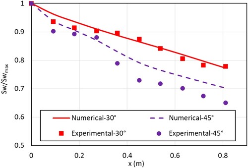
In order to further validate the numerical model, the results from the present numerical model were compared with the experimental data from the work of Clayton and Morsi (Clayton & Morsi, 1984). They measured the axial and tangential velocity profile in a straight annulus at different vane angles of a vortex generator. The internal diameter was 56 mm while the external was 109 mm, resulting in a radius ratio of 0.51. Most of the results were presented for the case with Re = 28700 and a radius ratio of 0.51. Therefore, these conditions have been used to further validate the numerical model. They reported an experimental accuracy of ±2%. Figure 8 shows the comparison of the normalized swirl number obtained from the numerical model with the experimental data for two different vane angles. The swirl number was normalized by diving it with the maximum swirl number. For the case of 30° vane angle, the average difference between the measured and numerical normalized swirl number was found to be 1.37% with a maximum of 2.83%. For the case of 45° vane angle, the average difference between the measured and normalized numerical swirl number was found to be 5.03% with a maximum of 7.18%. The difference between the experimental and numerical values can be attributed to the existence of a slightly non-uniform axial velocity profile at the inlet of the annulus in the experiment, for the case with 45° vane angle, while a uniform axial velocity profile along with a uniform tangential velocity profile was used as input flow condition for the numerical model.

Figure 8. Validation of the numerical model with experimental data for normalized swirl number (Sw/Sw_max) from Clayton and Morsi (1984).

Converging annulus

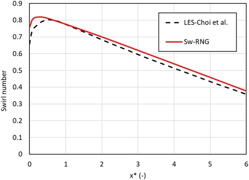
Figure 9 shows the variation of swirl number along the non-dimensional length. The flow Reynolds number was 12000, the radius ratio was γ = 7/14, the vane angle was 45° and the convergence gradient (β) of the annulus was 1/20. It can be seen from Figure 9 that the RNG k-ε turbulence model predicts the swirl number with good agreement in the developed region. The peak of the swirl number is slightly overpredicted in magnitude and shifted towards the swirler. A maximum deviation of 15% was obtained for the swirl number immediately after the end of the swirler. The high deviation, immediately after the swirler is due to the limitation of the steady-state two-equation model which can fail to capture the region of high turbulence (Wilcox, 1993) which occurs near the exit of the swirler. However, in the developed flow region the maximum deviation was around 2.3%.

Figure 9. Validation of swirl number along the varying cross-section annulus with results from Choi et al. (2018) (Re = 12000, θ = 45°, γ = 7/14, β = 1/20).

Results and discussion

This section presents and discusses the results relating to straight annulus, converging annulus, and diverging annulus geometry.

Straight annulus

In this section results pertinent to the straight annulus are presented. The effects of the Reynolds number on the flow, the radius ratio of the inner and the outer pipes and different vane angles are discussed. Figure 10 shows the schematic diagram of the straight annulus. The inner radius $R_i=8\text{mm}$ is kept constant for all the cases.

Figure 10. Cross-sectional schematic diagram of annular pipe.

The swirl number at any point along the length after the swirler is defined by Equation (7). The axial and tangential velocities at any point along the annulus are calculated by taking a mass average of the velocity along the cross-sectional surface. The radius ratio ($\gamma =R_i/R_{o,inlet}$) is defined based on the outer radius at the inlet of the annular cross-section geometry.

Effect of Reynolds number

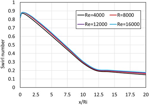
Figure 11 shows the effect of the Reynolds number on the swirl number of the flow throughout the annulus with γ = 8/16 (γ = R_i/R_o) and a swirler of vane angle, θ = 45°. Point 0 on the x-axis represents the point where the vanes of the swirler end. Using Equ.2 the swirl number calculated for the swirler is 0.78.

Figure 11. Effect of inlet Reynolds number on swirl number through the straight annulus (θ = 45°, γ = 8/16).

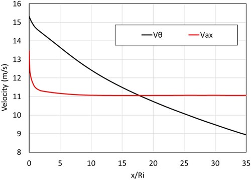
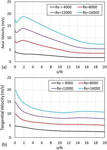
Immediately after the end of the vanes, a sudden increase in swirl number is observed (7%–9%), for the case of Re = 12000, the swirl number increases from 0.82 to 0.90 (9.17% increase). This increase is due to the reduction of the axial velocity component of the flow, as can be seen in Figure 12. The flow area inside the swirler is reduced due to the presence of the flat vanes. As the flow exits the swirler it needs to occupy the entire unobstructed area of the annulus, resulting in a decrease in the axial velocity component, which increases the swirl number initially (Choi et al., 2018). As the flow progresses through the annulus the swirl number decreases due to a decrease in the tangential velocity component of the flow. The swirl number in flow with higher $Re$ decreases at a slightly lower rate.

Figure 12. Axial (Vax) and tangential velocity (Vθ) component of the flow for Re = 12000 (θ = 45°, γ = 8/16).

A higher inlet Reynolds number for the flow leads to an increased swirl number. However, as it can be seen from the plots for$Re$ = 12000 to $Re=$16000, the increase in the Swirl number decreases and approaches an asymptote as the Reynolds number is increased. This suggests that there is no advantage to increasing the Reynolds number beyond a certain limit.

Effect of radius ratio

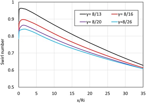
In this section, the effect of radius ratio (γ = R_i/R_o) is presented and discussed. Figure 13 shows the variation of swirl number along the axial direction of the flow, for different radius ratios. The radius ratios primarily affect the peak swirl number immediately after the swirler. The peak swirl number were 0.96, 0.90, 0.86 and 0.84 for the cases of γ = 8/13, 8/16, 8/20 and 8/26, respectively. With decreasing radius ratio, the decrease in the peak of the swirl number was also found to be reduced. When the diameter of the outer pipe is decreased i.e. γ is increased the cross-sectional area available for fluid transportation is decreased. This results in higher axial and tangential momentum of the flow. For instance, the axial and tangential velocity at the exit of the geometry with γ = 8/13 was 17.70 and 13.24 m/s, respectively, while that for the geometry with γ = 8/26 was 4.92 and 4.19 m/s, respectively. All the cases follow the pattern of axial and tangential velocity shown in Figure 12. The axial velocity continues to decrease monotonically while the tangential velocity remains mostly constant after the initial sharp decrease. After a distance of x/R_i= 35, the swirl number was found to be almost the same for all the cases, suggesting that as the radius of the outer pipe decreases, the rate of swirl decay increases.

Figure 13. Effect of radius ratio (γ) on swirl number through the straight annulus (θ = 45°, Re = 12000).

Effect of Vane angle

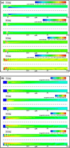
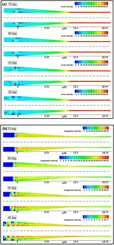
Figure 14 shows the variation of swirl number along the straight annulus with different swirler vane angles. Increasing the swirler vane angle significantly increases the swirl number of the flow through the straight annulus. For swirler vane angles of 60° and 70°, the swirl number immediately after the swirler decreases slightly before increasing unlike the cases with 30° and 45° swirlers. This is due to the formation of a small recirculation zone close to the inner pipe at the exit of the swirler. Figure 15 shows the contour plots of axial and tangential velocity components (in m/s) for straight annulus with different swirler vane angles. The recirculation zone with the 60° swirler is relatively very small while that with the 70° swirler is larger, thereby leading to swirl numbers that are lower than that with the 60° swirler close to the exit of the swirlers. The formation of a toroidal recirculation zone is one of the characteristics of a swirling flow (Gupta et al., 1984) due to the adverse pressure gradient in the axial and radial directions. The weekly swirling flows (at θ = 30° and 45°) experience low intensity of the adverse pressure gradient preventing flow separation near the swirler exit. As the swirling intensity increases strong axial and radial pressure gradients are experienced by the flow resulting in the formation of a toroidal recirculation zone (Gupta et al., 1984).

Figure 14. Effect of swirler vane angle (θ) on swirl number through the straight annulus (γ = 8/16, Re = 12000).

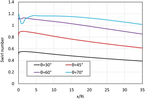
Figure 15. Contours of (a) axial and (b) tangential velocity along the straight annulus pipe with various vane angles (all velocities in m/s, γ = 8/16, Re = 12000).

The average increased in swirl was found to be 59% when the swirler vane angle is increased from 30° to 45°, by 38% when the swirler vane angle is increased from 45° to 60° and by 17% when the swirler vane angle is increased from 60° to 70°.

Based on the calculated swirl numbers for flow in a straight annular geometry a correlation to calculate the swirl number at non-dimensionalized length (x/R_i) greater than x/R_i = 0.05 and vane angle (θ) ≤ 60°, was developed and given below: (8) $\begin{array}{rl}{S}_w& =\frac{2}{3}\left[\frac{1-{\left(\gamma \right)}^3}{1-{\left(\gamma \right)}^2}\right]\tan \left(\theta \right)[1.4-0.176(\gamma )\phantom{\left(\frac{x}{R_i}\right)}\\ & +6\times {10}^{-6}\left(Re\right)+0.01\left(\frac{x}{R_i}\right)-0.24\tan \left(\theta \right)]\end{array}$(8) The R² of the above correlation was found to be 0.96. Using the above correlation, the swirl number can be predicted with an average error of 4%, with higher errors occurring in the cases for larger vane angles.

Converging cross-section annulus

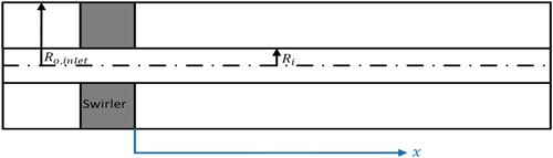
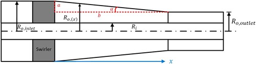
The effect of varying cross-section that converges along the length of the annulus is studied in this section. Figure 16 shows the schematic diagram of the converging annular geometry. The converging angle or the half cone angle with which the outer radius of the annulus decreases is given by: (9) $\alpha ={\tan }^{-1}\left(\text{β}\right)={\tan }^{-1}\frac{a}{b}$(9) The inner radius $R_i=8\text{mm}$ is kept constant for all the cases. The outer radius at any point along the axis of the geometry can be calculated as: (10) $R_{o,\left(x\right)}=R_{o,inlet}-x\text{β}$(10)

Figure 16. Cross-sectional schematic diagram of the converging annulus.

The swirl number at any point along the length after the swirler is defined as (11) $S_w\left(x\right)=\frac{2}{3}\left(\frac{1-{\left(\frac{R_i}{R_{o,x}}\right)}^3}{1-{\left(\frac{R_i}{R_{o,x}}\right)}^2}\right)\tan \left(\frac{V_{\theta }\left(x\right)}{V_{ax}\left(x\right)}\right)$(11)

Effect of Reynolds number

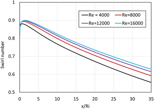
Figure 17 shows the effect of the Reynolds number on the swirl number along the nondimensionalized length of a converging annulus. The radius ratio (γ) used for the study was 8/16, the vane angle was 45° while the outer radius convergence gradient, β was 1/15, with b = 90 mm. At x/R_i= 11.25 (x = 90 mm), the geometry transitions to a straight annulus from a converging annulus geometry. The velocity at the inlet was varied to study the effect of the Reynolds number.

Figure 17. Effect of Reynolds Number on swirl number through converging annulus (θ = 45°, γ = 8/16, β = 1/15).

As the flow exits the swirler, the swirl number initially increases due to the decrease in the axial velocity as the flow area changes at the exit of the swirler. Thereafter in the converging part of the geometry (x/R_i< 11.25) the swirl number decreases at a significantly faster rate than that in a straight annulus (x/R_i< 11.25). This is due to the increase in axial velocity of the flow as a result of decreasing cross-sectional area. However, there is no significant effect of the Reynolds number on the swirl number in a converging geometry.

Effect of convergence gradient

Figure 18 shows the effect of the converging angle in terms of convergence gradient (β) which is calculated as given in Equation (9). $R_{o,inlet}$ was kept fixed in order to maintain a constant γ, $R_{o,utlet}$ was fixed as 10 mm while the length of the converging section ($b$, see Figure 16) was varied.

Figure 18. Effect of convergence gradient (β) on swirl number through converging annulus (θ = 45°, γ = 8/16, Re = 12000).

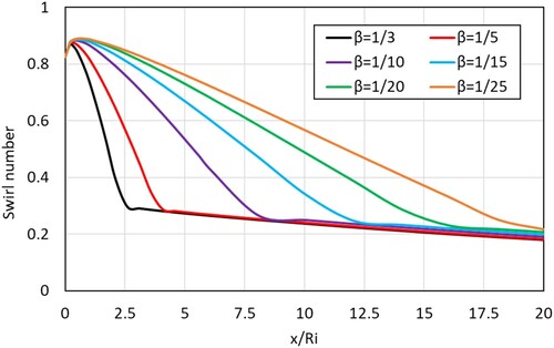
It can be seen that the rate of decrease in swirl number along the length of the converging annulus significantly depends on the convergence gradient (β). The steeper the gradient the quicker the swirl number decreases. This is attributed to the increase in axial velocity, which correspondingly leads to a decrease in tangential velocity. The flow accelerates quickly in the axial direction as the convergence gradient becomes steep. After the converging section the geometry transitions to the straight annular region. The position where this transition occurs depends upon the convergence gradient. For instance, in the case of the geometry with β = 1/3 the transition occurs at x/R_i = 2.5 while for β = 1/15 the transition occurs at x/R_i = 11.25. After the geometry transition from converging to straight the swirl number decays at a much slower rate in the straight annular section than in the converging annular section. The swirl number at the end of the converging cross-section varies between 0.30 and 0.21, with β = 1/3 having the highest swirl number and β = 1/25 having the lowest swirl number at the end of the converging section. The gradual convergence gradients have a lower swirl number at the outlet due to additional losses in swirl number arising from the increase in the length of the converging cross-sectional region.

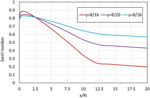
Effect of radius ratio

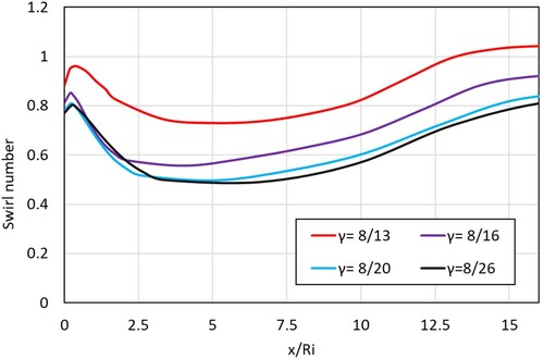
Figure 19 shows the effect of changing the radius ratio ($\gamma =R_i/R_{o,inlet}$) on the swirl number. The convergence gradient β was fixed at 1/15 by setting the length of the converging section ($b$, Figure 16) to 90 mm. It can be seen that using outer pipes of large diameter or in other words using smaller radius ratio geometries leads to a lower decay rate of swirl number in the converging section of the flow. This is contrary to what has been observed in the case of straight annular geometry. The presence of the converging section accelerates the flow by increasing the axial momentum at the expense of angular momentum. The axial velocity at the exit of the geometry with γ = 8/16 was 59 m/s while that in the geometry with γ = 8/26 was 9 m/s. Large diameter pipes have lower axial momentum flux due to which the swirl number decay along the length is reduced inside converging cross-sectional areas. The swirl number at the end of the converging section was found to be 0.23, 0.44 and 0.56 for γ = 8/16, 8/20 and 8/26, respectively. This suggests that wherever possible a large outer diameter pipe should be used in converging cross-sectional area geometry.

Figure 19. Effect of radius ratio (γ) on swirl number through converging annulus (θ = 45°, β = 1/15, Re = 12000).

Effect of Vane angle

Figure 20 shows the variation of swirl number in a converging annulus geometry with different swirler vane angles. Increasing the swirler vane angle results in a higher swirl number throughout the flow. For the cases of 30° and 45° swirlers, the swirl number inside the converging section decreases linearly. For the 60° and 70° swirlers, the decrease is non-linear resembling a quadratic polynomial. The increase of vane angle increases the axial momentum of the tangential flux resulting in higher swirl numbers at higher vane angles. The decrease in the ratio of axial to tangential velocity is linear, however, at higher vane angles the ratio of axial to tangential velocity is high, the tangent of which results in a non-linear decrease in swirl number at vane angles of 60° and 70°.

Figure 20. Effect of vane angle (θ) on swirl number through converging annulus (Re = 12000, γ = 8/16, β = 1/15).

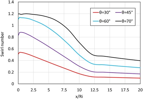
Figure 21 shows the axial and tangential velocity contours inside the converging annular geometry. For the case of the 70° swirler, a small recirculation zone can be seen near the exit of the swirler, this leads to a very small dip in swirl number, as seen in Figure 20. The average swirl number inside the converging section increased by 67% when the swirler vane angle is increased from 30° to 45°, by 37% when the swirler vane angle is increased from 45° to 60° and by 12% when the swirler vane angle is increased from 60° to 70°.

Figure 21. Contours of (a) axial and (b) tangential velocity along the converging annular geometry with various vane angles (all velocities in m/s, Re = 12000, γ = 8/16, β = 1/15).

Based on the calculated swirl numbers for flow in a converging annulus geometry a correlation to calculate the swirl number at non-dimensionalized length (x/R_i) for x/R_i > 0.05, was developed and is presented as Equation (12). Two sets of coefficients are used to provide good prediction; the first set of coefficients are to be used when predicting swirl number in converging sections while the second set of correlations are to be used in the straight annular section after the converging geometry (Table 2). (12) $S_w=S_{w,ref}\left[\begin{array}{l}{a}_0+a_1{Re}^{\ast }+a_2{\text{β}}^{\ast }+a_3{X}^{\ast }+a_4\gamma \\ +a_5\tan \theta +a_6{\gamma }^2+a_7{\left({\text{β}}^{\ast }\right)}^2\\ +a_8{\left(X^{\ast }\right)}^2+a_9{\tan }^2\theta +a_{10}{\text{β}}^{\ast }{X}^{\ast }\\ +a_{11}{X}^{\ast }\tan \theta +a_{12}\gamma X^{\ast }\end{array}\right]$(12) where $R{e}^{\ast }=\ln \left(R{e}_{inlet}\right)$, ${\text{β}}^{\ast }=\ln \left(\text{β}\right)$ and $X^{\ast }=\ln \left(\frac{x}{R_i}\right)$.

$S_{w,ref}$ is the reference swirl number. For flow in the converging section $S_{w,ref}$ is calculated using Equation (2). For the straight annular section after the converging geometry $S_{w,ref}$ is equal to the swirl number at the end of the converging section.

Diverging cross-section annulus

The effect of varying cross-section that diverges along the length of the annulus is studied in this section. Figure 22 shows the schematic diagram of the diverging annular geometry. The diverging angle or the half cone angle with which the outer radius of the annulus increases is given by Equation (9). The inner radius $R_i=8\text{mm}$ is kept constant for all the cases. The outer radius at any point along the axis of the geometry can be calculated as: (13) $R_{o,\left(x\right)}=R_{o,inlet}+x\text{β}$(13)

Figure 22. Cross-sectional schematic diagram of the diverging annulus.

The swirl number at any point along the length after the swirler is defined using Equation (11).

Effect of Reynolds number

Figure 23 shows the effect of variation of inlet Reynolds number inside a diverging annular cross-section. The diverging section of the geometry has a length of $b$ = 9 cm from where on a straight annulus follows. The swirl number for all cases increases for a short length and then decreases before increasing again. The swirl number continues to increase even in the straight annulus for some distance. Another point worth mentioning is that the higher the Reynolds number, the swirl number dips to a lower value, taking a longer distance to recover. Figure 24 shows the contour plots for axial and tangential velocities at different inlet Reynolds numbers. At Re = 4000, the flow separates from the inner tube and a recirculation zone can be seen starting at x/R_i= 2. The diverging geometry exacerbates the axial and radial pressure gradient, leading to flow separation from the inner tube resulting in the development of a toroidal recirculation zone even with a vane angle of 45°, which was not observed in a straight annular geometry with a vane angle of 45°. At a higher inlet Reynolds number, the recirculation zone can be observed immediately after the swirler at around x/R_i= 0.2 from the swirler exit.

Figure 25 shows the mass-weighted axial and tangential velocity along the diverging annular geometry. The toroidal recirculation zone chokes the flow leading to an increase in the axial velocity after the swirler for Re > 4000. A small increase in axial velocity is observed far downstream of the swirler. The axial velocity first decreases between x/R_i 0–0.2 and then increases sharply between x/R_i 0.2–1.8, for Re > 4000. At x/R_i= 1.8, the radius of the diverging annulus has expanded enough such that it could compensate for the decreased axial flow area due to the presence of the recirculation zone. Therefore, at this point, the axial velocity starts to decrease. The axial velocity continues to decrease even after the end of the diverging annular area because the area occupied by the recirculation zone also decreases. At Re = 4000 a very small increase in axial velocity is observed between x/R_i = 2–4.

Figure 23. Effect of Reynolds Number on swirl number through the diverging annulus (θ = 45°, γ = 8/16, β = 1/15).

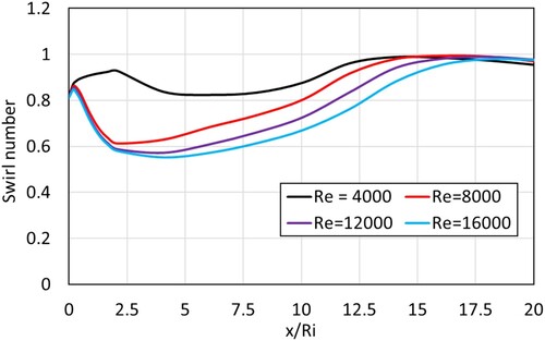
Figure 24. Contours of (a) axial and (b) tangential velocity along the diverging annular geometry for different Re (all velocities in m/s; θ = 45°, γ = 8/16, β = 1/15).

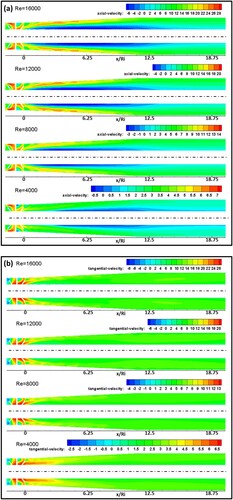
Figure 25. (a) Axial and (b) tangential velocity along the diverging annular geometry for different Reynolds number (θ = 45°, γ = 8/16, β = 1/15).

The tangential velocity decreases, non-linearly, throughout the diverging section and reaches nadir at around x/R_i= 11.25 with a small increase thereafter for Re > 4000. This is attributed to the presence of a small region of the recirculation zone extending into the straight annular region of the geometry.

The flow with a higher Reynolds number experiences a longer recirculation zone, due to which it takes longer to recover the swirl number in comparison with the cases with a lower Reynolds number. The recovered swirl number reaches a value between 0.98 and 0.99. The swirl number decay in the straight annulus section of the geometry is much slower, thus, the swirl numbers at the exit of the geometry are closer to each other as shown in Figure 23. The swirl number at the exit for Re = 4000, 8000, 12000 and 16000 was 0.95, 0.97, 0.98 and 0.98 respectively.

Effect of divergence gradient

In this section, the effect of divergence gradient (β) is presented and discussed. The outer diameter at the outlet ($R_{o,outlet}$) was fixed at 44 mm. The diverging gradient was varied by changing the length of the diverging annular geometry. Figure 26 shows the effect of β on the swirl number along the axis of the diverging annular geometry. For cases with β = 1/3–1/23, the swirl number first increases sharply close to the exit of the swirler i.e. up till x/R_i = 0.2, then it decreases suddenly due to the formation of toroidal recirculation zone, followed by a recovery of swirl number. For cases with β = 1/23-1/25, the swirl number does not start to fall immediately because the toroidal recirculation zone in these cases is shifted downstream. The location of the recirculation zone is further shifted downstream with a decrease in β as can be seen in Figure 27, which shows the contour plot of axial and tangential velocity for different β.

Figure 26. Effect of gradient (β) on swirl number through diverging annulus (θ = 45°, γ = 8/16, Re = 12000).

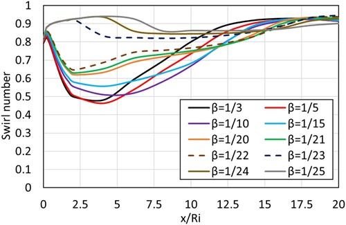
Figure 27. Contours of (a) axial and (b) tangential velocity along the diverging annular geometry for different values of β (all velocities in m/s; θ = 45°, γ = 8/16, Re = 12000).

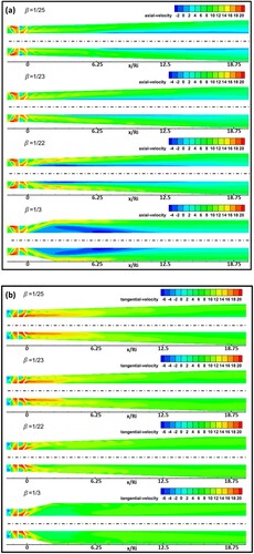
The formation of the recirculation zone can be attributed to the diverging cross-section of the swirling flow itself. The shift of the recirculation zone downstream, for cases with β = 1/23–1/25, suggests that it is the diverging geometry that causes adverse axial and radial pressure gradients at the exit of the swirler resulting in the formation of a toroidal recirculation zone near the surface of the inner pipe immediately after the swirler. The strength of the recirculation zone decreases with the decrease in the divergence gradient.

Effect of radius ratio

Figure 28 depicts the effect of radius ratio on the swirl number in a diverging annular geometry. Similar to the behavior observed in the case of straight annular geometry, a higher radius ratio results in a higher swirl number. As the outer diameter of the pipe is increased, i.e. γ is decreased the area available for fluid transportation is increased resulting in lower axial and tangential momentum. However, contrary to the case with the straight annulus where the tangential velocity remains almost uniform throughout the axial distance, after an initial drop the tangential velocity drops smoothly as seen previously in Figure 25(b). The higher axial and tangential momentum results in a higher swirl number for γ = 8/13. The swirl number for the cases 8/20 and 8/26 are almost the same suggesting that there is not much appreciable decrease in swirl number on increasing the outer diameter beyond a certain limit.

Figure 28. Effect of γ on swirl number through the diverging annulus (θ = 45°, β = 1/15, Re = 12000).

Effect of Vane angle

The effect of the swirler vane angle on the swirl number through the diverging annular geometry is shown in Figure 29 while Figure 30 depicts the contours of axial and tangential velocity in the annular diverging geometry with different vane angles. The higher the vane angle the higher the swirl number is obtained in the annular geometry. For vane angles 45°–70° the swirl number decreases and then it rises again, while for the vane angle of 30°, an opposite phenomenon is observed, where the swirl number increases in the diverging region (x/R_i < 11.25) of the geometry and then it decreases in the straight section of the geometry.

Figure 29. Effect of vane angle (θ) on swirl number through diverging annulus (Re = 12000, γ = 8/16, β = 1/15).

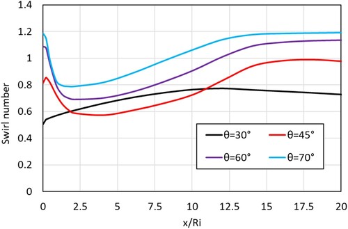
Figure 30. Contours of (a) axial and (b) tangential velocity along the diverging annular geometry for different swirler vane angles (all velocities in m/s; Re = 12000, γ = 8/16, β = 1/15).

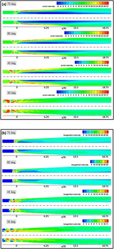
For the cases with θ > 30°, the increased swirl intensity results in adverse axial and radial pressure gradient leading to the development of a toroidal recirculation zone at the exit of the swirler. The axial and tangential velocities vary in the same manner as previously discussed. Figure 31 shows the axial and tangential velocities along the diverging annular geometry. Higher vane angles lead to higher axial and tangential velocities. The increase in axial velocity after the swirler with vane angle θ > 30° is due to the reduction in the cross-sectional area, which is caused by the presence of a toroidal recirculation zone. With an increase in vane angle, the recirculation zone gets stronger and bigger. As the recirculation zone grows with an increase in vane angle, it decreases the cross-sectional area available for the flow to pass through. This phenomenon causes the flow to accelerate, as a result of which its axial velocity increases significantly between x/R_i = 0.25 and 2.1, after which the axial velocity decreases at a relatively gradual pace. The axial velocity reaches a peak value at x/R_i = 2.1, 1.7 and 1.3 for vane angles of 45°, 60° and 70°, respectively. Between x/R_i = 0.25 and 2.5 the tangential velocity also decreases significantly, which is attributed to the increase in the associated axial velocity. The decrease in tangential velocity and increase in axial velocity cause the swirl number to drop between x/R_i = 0 and 2.5. After reaching the peak, the axial velocity continues to decrease gradually while the decrease in the tangential velocity beyond x/R_i = 5 becomes very small, which is eventually approaching an asymptote at around x/R_i = 7.5. This behavior results in the recovery of the swirl number as the tangential velocity becomes greater than axial velocity.

Figure 31. (a) Axial and (b) tangential velocity along the diverging annular geometry for different vane angles (Re = 12000, γ = 8/16, β = 1/15).

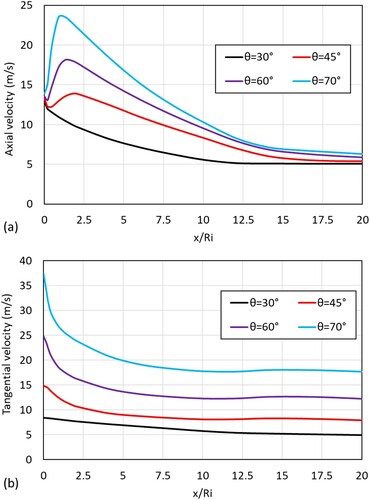
Due to the higher vane angles, which provide a higher tangential momentum to the initial flow, the tangential velocity for cases with θ > 30° is higher than the axial velocity. As a result, the swirl number at the exit of the diverging annulus is higher for cases with higher vane angles.

. The variation of axial and tangential velocity along the geometry with θ = 30° is different as shown in Figure 31. Due to the absence of a toroidal recirculation zone, the tangential velocity decreases linearly while the axial velocity decreases with a parabolic-like profile due to the increase in the cross-sectional area, which is a function of radius squared. The decrease in axial velocity is more significant than the decrease in tangential velocity. As a result, the swirl number increases in the diverging annular geometry with θ = 30°.

The average swirl number inside the diverging section increased by 7% when the swirler vane angle is increased from 30° to 45°, by 18.7% when the swirler vane angle is increased from 45° to 60° and by 12% when the swirler vane angle is increased from 60° to 70°. This suggests that inside the diverging section the change in the area plays a much more important role than the swirler vane angle.

Based on the calculated swirl numbers for flow in a diverging annulus a correlation to calculate the swirl number at non-dimensionalized length (x/R_i) for x/R_i > 0.05, was developed and is presented as Equ. 14. The coefficient used in the correlation is presented in Table 3. $S_{w,ref}$ is the reference swirl number which is calculated using Equ. 2. (14) $S_w=S_{w,ref}\left[\begin{array}{l}{a}_1{Re}^{\ast }+a_2{\text{β}}^{\ast }+a_3{X}^{\ast }+a_4\tan \theta +a_5\gamma \\ +a_6{\left({\text{β}}^{\ast }\right)}^2+a_7{\left(X^{\ast }\right)}^2+a_8{\tan }^2\theta \\ +a_9{\text{β}}^{\ast }{Re}^{\ast }+a_{10}{\text{β}}^{\ast }{X}^{\ast }\end{array}\right]$(14) where $R{e}^{\ast }=\ln \left(R{e}_{inlet}\right)$, ${\text{β}}^{\ast }=\ln \left(\text{β}\right)$ and $X^{\ast }=\ln \left(\frac{x}{R_i}\right)$.

Conclusion

Swirl flow inside annular geometries with straight and varying cross-sectional areas is examined using computational fluid dynamics (CFD). Effect of Reynolds number and geometric parameters such as radius ratio, swirler vane angles and cone angles of converging and diverging annular geometries were studied. The following conclusions can be drawn from the study:

1. In all cases, immediately after the swirler, the swirl number was found to increase suddenly due to a decrease in axial velocity. After reaching a peak the swirl number decreases monotonically in the case of the straight annulus and converging annular geometry. In the case of the diverging annulus with θ > 30°, the swirl number after a peak initially decreases and then increases again. This was due to the formation of a recirculation zone near the inner pipe in case of diverging annuli. For θ = 30°, in the diverging annular geometry, the swirl number increases in the diverging region of the geometry due to increasing cross sectional area which reduces the axial velocity much more than the tangential velocity.

2. Reynolds number was found to increase the peak swirl number in straight and diverging cross-sectional geometries while no significant effect of Reynolds number was observed in converging cross-sectional geometry.

3. Decreasing the radius ratio increased the peak swirl number significantly in all the three types of geometries studied. In the case of a straight annular pipe, although a higher swirl number was observed initially at a lower radius ratio, the effect on swirl number becomes negligible after a certain distance. In the case of diverging annular geometry, the increase in swirl number diminishes as the radius ratio is decreased.

4. The effect of the swirler vane angle on the swirl number inside the annular geometries was also studied. It was found that increasing the vane angle increased the swirl number in all cases. At higher vane angles of 60° and 70°, a recirculation zone is developed near the exit of the swirler. This leads to a non-linear decay rate of swirl inside the annular geometries with varying cross-sectional areas.

5. Using small cone angles was found to lead to a lower swirl decay rate in converging and diverging nozzles.

Acknowledgements

For computer time, this research used the resources of the Supercomputing Laboratory at King Abdullah University of Science & Technology (KAUST) in Thuwal, Saudi Arabia. The support provided by the King Abdullah City for Atomic and Renewable Energy (K. A. CARE) is also highly acknowledged.

Disclosure statement

No potential conflict of interest was reported by the author(s).

Additional information

Funding

This work was supported by DROC of King Fahd University of Petroleum and Minerals (KFUPM), Dhahran Saudi Arabia [grant number DF181008].

References

- Abo-Elfadl, S., & Abd El-Sabor Mohamed, A. (2018). The effect of the helical inlet port design and the shrouded inlet valve condition on swirl generation in diesel engine. Journal of Energy Resources Technology, 140(3), 1–9. https://doi.org/10.1115/1.4037941
- Agarwal, A., & Mthembu, L. (2020). CFD analysis of conical diffuser under swirl flow inlet conditions using turbulence models. Materials Today: Proceedings, 27(2), 1350–1355. https://doi.org/10.1016/j.matpr.2020.02.621
- Alam, H. S., Redhyka, G. G., Sugiarto, A. T., Salim, T. I., & Mardhiya, I. R. (2018). Design and performance of swirl flow microbubble generator. International Journal of Engineering and Technology(UAE), 7(4), 66–69. https://doi.org/10.14419/ijet.v7i4.40.24077
- Algifri, A. H., Bhardwaj, R. K., & Rao, Y. V. N. (1988). Eddy viscosity in decaying swirl flow in a pipe. Applied Scientific Research, 45(4), 287–302. https://doi.org/10.1007/BF00457063
- Aliyu, M., Nemitallah, M. A., Said, S. A., & Habib, M. A. (2016). Characteristics of H2-enriched CH4eO2 diffusion flames in a swirl-stabilized gas turbine combustor: Experimental and numerical study. International Journal of Hydrogen Energy, 41(44), 20418–20432. https://doi.org/10.1016/j.ijhydene.2016.08.144
- Biswas, G., & Som, S. K. (1986). Coefficient of discharge and spray cone angle of a pressure nozzle with combined axial and tangential entry of power-law fluids. Applied Scientific Research, 43(1), 3–22. https://doi.org/10.1007/BF00385725
- Carlanescu, R., Prisecaru, T., Prisecaru, M., & Soriga, I. (2018). Swirl injector for premixed combustion of hydrogen-methane mixtures. Journal of Energy Resources Technology, 140(7), 7. https://doi.org/10.1115/1.4039267
- Carlos Berrio, J., Pereyra, E., & Ratkovich, N. (2018). Computational fluid dynamics modeling of gas-liquid cylindrical cyclones, geometrical analysis. Journal of Energy Resources Technology, 140(9), 1–14. https://doi.org/10.1115/1.4039609
- Chang, C., Merkle, C., State, P., Promenade, L. E., Chang, C., & Merkle, C. L. (1989). Viscous Swirling Nozzle Flow. 27th Aerospam Sciences Meeting. American Institute of Aeronautics and Astronaurics.
- Chiaverhi, M. J., Malecki, M. J., Sauer, J. A., & Knuth, W. H. (2002). Vortex combustion chamber development for future liquid rocket engine applications. American Institute of Aeronautics and Astronautics.
- Choi, J., Jung, E., Kang, S., & Do, H. (2018). Modeling swirl decay rate of turbulent flows in annular swirl injectors. AIAA Journal, 56(12), 4910–4926. https://doi.org/10.2514/1.J057236
- Clayton, B. R., & Morsi, Y. S. M. (1984). Determination of principal characteristics of turbulent swirling flow along annuli. International Journal of Heat and Fluid Flow, 5(4), 195–203. https://doi.org/10.1016/0142-727X(84)90051-1
- Cloos, F. J., & Pelz, P. F. (2019). Experimental investigation of the swirl development at the inlet of a coaxial rotating diffuser or nozzle. Journal of Fluids Engineering, 141(4), 041107. https://doi.org/10.1115/1.4042095.
- Degenève, A., Jourdaine, P., Mirat, C., Caudal, J., Vicquelin, R., & Schuller, T. (2019). Effects of a diverging cup on swirl number, flow pattern, and topology of premixed flames. Journal of Engineering for Gas Turbines and Power, 141(3), 1–13. https://doi.org/10.1115/1.4041518
- Dinesh, K. K. J. R., Richardson, E. S., Van Oijen, J. A., Luo, K. H., & Jiang, X. (2015). The scalar structure of turbulent oxy-fuel non-premixed flames. Physics Procedia, 66, 305–308. https://doi.org/10.1016/j.egypro.2015.02.066
- Elkhoury, M. (2017). On eddy viscosity transport models with elliptic relaxation. Journal of Turbulence, 18(3), 240–259. https://doi.org/10.1080/14685248.2016.1272758
- Erdal, F. M., & Shirazi, S. A. (2004). Local velocity measurements and computational fluid dynamics (CFD) simulations of swirling flow in a cylindrical cyclone separator. Journal of Energy Resources Technology, 126(4), 326–333. https://doi.org/10.1115/1.1805539
- Fiorina, B., Mercier, R., Kuenne, G., Ketelheun, A., Avdić, A., Janicka, J., & Kempf, A. (2015). Challenging modeling strategies for LES of non-adiabatic turbulent stratified combustion. Combustion and Flame, 162(11), 4264–4282. https://doi.org/10.1016/j.combustflame.2015.07.036
- Franke, L. L. C., Chatzopoulos, A. K., & Rigopoulos, S. (2017). Tabulation of combustion chemistry via Artificial Neural Networks (ANNs): Methodology and application to LES-PDF simulation of Sydney flame L. Combustion and Flame, 185, 245–260. https://doi.org/10.1016/j.combustflame.2017.07.014
- Granados-Ortiz, F. J., Leon-Prieto, L., & Ortega-Casanova, J. (2021). Computational study of the application of Al2O3 nanoparticles to forced convection of high-Reynolds swirling jets for engineering cooling processes. Engineering Applications of Computational Fluid Mechanics, 15(1), 1–22. https://doi.org/10.1080/19942060.2020.1845805
- Guillaume, D. W., & Judge, T. A. (2004). Improving the efficiency of a jet pump using a swirling primary jet. Review of Scientific Instruments, 75(2), 553–556. https://doi.org/10.1063/1.1638873.
- Gupta, A. K., Lilley, D. G., & Syred, N. (1984). Swirl flows. Abacus Press.
- Habib, M. A., Ben-Mansour, R., Badr, H. M., Ahmed, S. F., & Ghoniem, A. F. (2012). Computational fluid dynamic simulation of oxyfuel combustion in gas-fired water tube boilers. Computers and Fluids, 56, 152–165. https://doi.org/10.1016/j.compfluid.2011.12.009
- Herff, S., Niemöller, A., Meinke, M., & Schröder, W. (2021). LES of a turbulent swirl flame using a mesh adaptive level-set method with dynamic load balancing. Computers and Fluids, 221, 104900. https://doi.org/10.1016/j.compfluid.2021.104900.
- Hogg, S., & Leschziner, M. A. (1989). Computation of highly swirling confined flow with a Reynolds stress turbulence model. AIAA Journal, 27(1), 57–63. https://doi.org/10.2514/3.10094
- Islam, S. M., Tanvir Khan, M., & Ahmed, Z. U. (2020). Effect of design parameters on flow characteristics of an aerodynamic swirl nozzle. Progress in Computational Fluid Dynamics, 20(5), 249–262. https://doi.org/10.1504/PCFD.2020.109912
- Jawarneh, A. M., & Vatistas, G. H. (2006). Reynolds stress model in the prediction of confined turbulent swirling flows. Journal of Fluids Engineering, 128(6), 1377–1382. https://doi.org/10.1115/1.2354530
- Khan, M. T., Islam, S. M., & Ahmed, Z. U. (2020). Near-wall and turbulence behavior of swirl flows through an aerodynamic nozzle. Journal of Engineering Advancements, 01(02), 43–52. https://doi.org/10.38032/jea.2020.02.003
- Koh, H., Kim, D., Jung, K., Park, J., Yoon, Y., Koh, H., & Yoon, Y. (2001). The Effects of Swirler Geometry on the Performance of Gas Turbine Combustor Using Planar Imaging Technique. Retrieved from 37th AIAA/ASME/SAE/ASEE Joint Propulsion Conference & Exhibit 8–11 July 2001/Salt Lake City, Utah The Effects of Swirler Geo.
- Leclaire, B., Jacquin, L., & Sipp, D. (2005). Effects of a contraction on a uniformly rotating flow. 4th AIAA Theoretical Fluid Mechanics Meeting, (June), 1–12. https://doi.org/10.2514/6.2005-4677.
- Lee, J., Lee, H., Park, H., Cho, G. H., Kim, D., & Cho, J. (2021). Design optimization of a vane type pre-swirl nozzle. Engineering Applications of Computational Fluid Mechanics, 15(1), 164–179. https://doi.org/10.1080/19942060.2020.1847199
- Lineberry, C. W. (1968). A study of swirling air flow in a converging nozzle.
- Marzouk, O. A., & David Huckaby, E. (2010). Simulation of a swirling gas-particle flow using different k-epsilon models and particle-parcel relationships. Engineering Letters, 18(1).
- Masri, A. R. (2015). Partial premixing and stratification in turbulent flames. Proceedings of the Combustion Institute, 35(2), 1115–1136. https://doi.org/10.1016/j.proci.2014.08.032
- Menter, F. R. (1994). Two-equation eddy-viscosity turbulence models for engineering applications. AIAA Journal, 32(8), 1598–1605. https://doi.org/10.2514/3.12149
- Namet-Allah, A., & Birk, A. M. (2014). Numerical and experimental study of swirling flow in a short annular to round diffuser/nozzle. Proceedings of the ASME Turbo Expo, 1A, 1–14. Paper no. GT2014-26486. https://doi.org/10.1115/GT2014-26486
- Norton, D. J., Farquhar, B. W., & Hoffman, J. D. (1969). Analytical and experimental investigation of swirling flow in nozzle. AIAA Journal, 7(10), 1992–2000. https://doi.org/10.2514/3.5493
- Pang, X., Wang, C., Yang, W., Fan, H., Zhong, S., Zheng, W., & Chen, S. (2022). Numerical simulation of a cyclone separator to recycle the active components of waste lithium batteries. Engineering Applications of Computational Fluid Mechanics, 16(1), 937–951. https://doi.org/10.1080/19942060.2022.2053343
- Ranga Dinesh, K. K. J., Van Oijen, J. A., Luo, K. H., & Jiang, X. (2014). Near-field local flame extinction of oxy-syngas non-premixed jet flames: A DNS study. Fuel, 130, 189–196. https://doi.org/10.1016/j.fuel.2014.04.011
- Shakeel, M. R., Sanusi, Y. S., & Mokheimer, E. M. A. (2018). Numerical modeling of oxy-methane combustion in a model gas turbine combustor. Applied Energy, 228, 68–81. https://doi.org/10.1016/j.apenergy.2018.06.071.
- Sheikholeslami, M., Gorji-Bandpy, M., & Ganji, D. D. (2015). Review of heat transfer enhancement methods: Focus on passive methods using swirl flow devices. Renewable and Sustainable Energy Reviews, 49, 444–469. https://doi.org/10.1016/j.rser.2015.04.113
- Sui, C., Zhang, J., Zhang, L., Hu, X., & Zhang, B. (2021). Large eddy simulation of premixed hydrogen-rich gas turbine combustion based on reduced reaction mechanisms. Engineering Applications of Computational Fluid Mechanics, 15(1), 798–814. https://doi.org/10.1080/19942060.2021.1918581
- Sweeney, M. S., Hochgreb, S., Dunn, M. J., & Barlow, R. S. (2012). The structure of turbulent stratified and premixed methane/air flames II: Swirling flows. Combustion and Flame, 159(9), 2912–2929. https://doi.org/10.1016/j.combustflame.2012.05.014
- Syred, N., & Beér, J. M. (1974). Combustion in swirling flows: A review. Combustion and Flame, 23(2), 143–201. https://doi.org/10.1016/0010-2180(74)90057-1
- Taylor, G. I. (1950). The boundary layer in the converging nozzle of a swirl atomizer. Quarterly Journal of Mechanics and Applied Mathematics, 3(2), 129–139. https://doi.org/10.1093/qjmam/3.2.129
- Van Maele, K., Merci, B., & Dick, E. (2003). Comparative study of k-ε turbulence models in inert and reacting swirling flows. 33rd AIAA Fluid Dynamics Conference and Exhibit, 1–10. https://doi.org/10.2514/6.2003-3744.
- Vaziri, B. M., & Shahsavand, A. (2015). Optimal selection of supersonic separators inlet velocity components via maximization of swirl strength and centrifugal acceleration. Separation Science and Technology, 50(5), 752–759. https://doi.org/10.1080/01496395.2014.958782
- Wilcox, D. C. (1993). Comparison of two-equation turbulence models for boundary layers with pressure gradient. AIAA Journal, 31(8), 1414–1421. https://doi.org/10.2514/3.11790
- Yan, T., Qu, J., Sun, X., Chen, Y., Hu, Q., & Li, W. (2020). Numerical evaluation on the decaying swirling flow in a multi-lobed swirl generator. Engineering Applications of Computational Fluid Mechanics, 14(1), 1198–1214. https://doi.org/10.1080/19942060.2020.1816494
- Yang, S. L., Siow, Y. K., Peschke, B. D., & Tacina, R. R. (2003). Numerical study of nonreacting gas turbine combustor swirl flow using Reynolds stress model. Journal of Engineering for Gas Turbines and Power, 125(3), 804–811. https://doi.org/10.1115/1.1560706
- Zhao, H., Wang, F., Wang, C., Chen, W., Yao, Z., Shi, X., & Zhong, Q. (2021). Study on the characteristics of horn-like vortices in an axial flow pump impeller under off-design conditions. Engineering Applications of Computational Fluid Mechanics, 15(1), 1613–1628. https://doi.org/10.1080/19942060.2021.1985615