From μCT data to CFD: an open-source workflow for engineering applications

Abstract

The generation of high-quality volume meshes out of µCT data can be a challenging task that is mandatory to perform CFD simulations of fluid flows within or around scanned objects. Despite the growing relevance of CT-based CFD simulations, there is still a lack of a standardized, free-to-use workflow. In this work, an open-source based workflow is presented, which covers all steps from the CT image stack to a volume mesh in the end. The software packages ImageJ, ParaView, and Blender are used for surface reconstruction and processing of µCT data; resulting meshes are evaluated regarding geometric parameters, surface fidelity, and used memory. For volume meshing, the mesh generator snappyHexMesh implemented in OpenFOAM is used. A detailed description of this workflow is provided in the Supplementary Materials. We demonstrate how potential pitfalls and shortcomings can be avoided and how surface smoothing is especially important to preserve the surface area of scanned objects. We use CT data of a 10 ppi open cell foam to illustrate that data decimation can reduce the required time for the volume meshing by up to 45% and RAM up to 75%. The resulting meshes are used to simulate flow fields and heat transport with a surface heat source. The resulting temperature fields show that differences in the surface area and recesses in an unsmoothed mesh can affect the outcome of heat transport simulations, highly relevant for reactive CFD simulations. The results highlight the quality of our workflow’s outcome, which can help engineers that rely on CT reconstruction processes, also for other applications.

KEYWORDS:

• Open-cell foam
• periodic open-cell structure
• surface reconstruction
• volume meshing
• OpenFOAM

List of abbreviations

CFD	=	Computational Fluid Dynamics
DICOM	=	Digital Imaging and Communication in Medicine
POCS	=	Periodic Open Cell Foams
MC	=	Marching Cubes
µCT	=	Micro-Computed Tomography
Mesh P	=	Processed Mesh
Mesh UP	=	Unprocessed Mesh
NMR	=	Nuclear Magnetic Resonance
NURBS	=	Non-Uniform Rational B-Spline
ppi	=	pores per inch
RAM	=	Random-Access Memory
sHM	=	snappyHexMesh
STL	=	Standard Tessellation Language
VoMaC	=	Volumetric Marching Cubes

1. Introduction

Computational Fluid Dynamics (CFD) is a prominent method in the engineering community to obtain deep insights into flow, temperature, and/or species fields in and around objects of interest in single and multi-phase environment. While in the first stages of CFD modeling the objects were trivial and generated manually [e.g. flow around bluff bodies (Krajnovic & Davidson, 2000)], nowadays it is possible to investigate complex structures like porous materials (Wood et al., 2020). The increasing object complexity requires the inventions of novel tools to digitize the geometry. One possible way is to use surrogate structures based on geometrical parameters of the real object. For example, Voroni tessellations are frequently used to generate digital replicas of Open Cell Foams (OCF) (Wehinger et al., 2016) and most recently an open-source workflow to generate such structures was presented (Agostini et al., 2022). However, such surrogates are only applicable if local phenomena in the real object are not important. To implement a real object into a CFD model, it must be scanned and resulting data must be processed properly. Possible methods of collecting the geometrical data are laser and radar scanners, sonar, Nuclear Magnetic Resonance (NMR) or X-Ray Computer Tomography (CT) (Rychlik et al., 2004). The latter is by far the most popular. The combination of CT with CFD simulations is referred to as image-based CFD.

The first field to combine CT with CFD was biomedical engineering. In 1993, first attempts were made to investigate the blood flow of a stenosed arterial bifurcation (Tasciyan et al., 1993). Since then, numerous works have been published regarding the cardiovascular system (Kagadis et al., 2008; Qiu et al., 2018; Tippe et al., 1999) and the respiratory tract (Inthavong et al., 2009; Nowak et al., 2003; Quadrio et al., 2016; Shukla et al., 2020; Tabe et al. 2021). It took many years for image-based CFD to find its way into other engineering disciplines. Apart from a pioneering work of Menegazzi and Trapy (1997), who analysed an engine cooling system using a combination of CFD and CT data in 1997, frequent usage started only in the late 2000s (Tabor et al., 2008). Over the last decade, extensive research has been carried out based on image-based CFD, including works on droplet spreading in porous media (Aboukhedr et al., 2017), electrolyte flow in batteries (Emmel et al., 2020), conjugate heat transfer in monolithic catalyst supports (Sinn et al., 2020), and even reaction simulations in catalytic reactors (Dong et al., 2018). The application fields grow as rapidly as the need of specific knowledge on the whole process towards the simulation of real objects.

Converting CT data to volume meshes, which are the basis for Finite Volume Method-based CFD, is by no means trivial. The amount of data can be immense and thus challenging to handle. This is especially true for fine geometries like porous media, which is why data reduction is of utmost importance. Hence, the pre-processing, which is already considered as one of the most time consuming steps in CFD simulations (Ali et al., 2019), becomes even more challenging. Surprisingly, although lots of knowledge and methods for meshing of CT data are known (see Chapter 2), the meshing procedure for these complex geometries is still very time consuming and prone to error. The main reason is probably a lack of standardised meshing workflows that can deal with complex geometries and are easy to use for CFD engineers, who are no experts in digital image processing and surface reconstruction.

This paper presents a straightforward an ‘easy-to-use' workflow for the processing of CT image sequences into sound volume meshes, which can be used as the discretised calculation domain for CFD simulations. The workflow is based on open-source software prominent in the scientific community. Our aim is to show a standardised way to generate a sound mesh, both to facilitate the pre-processing and overcome additional challenges of image-based CFD. Furthermore, the influence of the process steps on the morphology of sample objects is shown as well as the influence of smoothing surface meshes on CFD results of conjugate heat transfer simulations in an OCF reactor. The workflow is explained in detail throughout this manuscript and the Supplementary Materials. Furthermore, utilized STL files and simulation cases are uploaded to a repository. The following key questions will be addressed in the present manuscript:

• Is it reasonable to use uncompressed CT data for meshing?

• How is volume and surface preservation dependent on smoothing?

• Are there significant differences in CFD results between smoothed and unsmoothed meshes?

2. Theory

Several works have been published describing methods to either create proper surface meshes or to create volume meshes directly out of image stacks of CT scans (Inthavong et al., 2009; Manmadhachary et al., 2016; Wang et al. 2010; Young et al., 2008). Almost all the research on converting CT data to digital meshes was done in the field of biomedical engineering, which is why the starting point in many cases is Digital Imaging and Communication in Medicine (DICOM) data. These files contain the CT data as image stacks or voxel data, the basis for further processing. In the following, common meshing methods are grouped into direct and indirect methods (visualized in Figure 1).

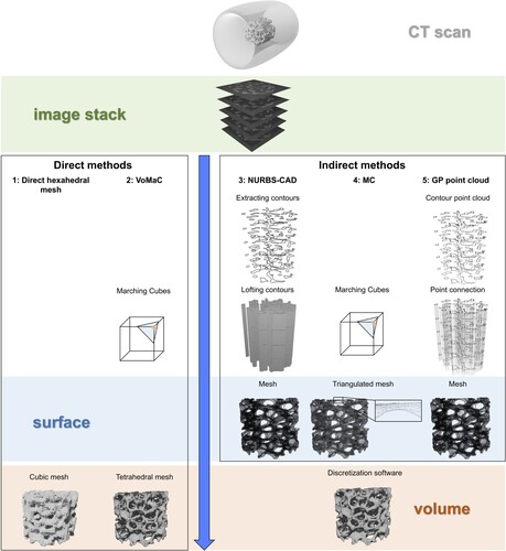
Figure 1. Possible techniques to create volume meshes from CT data. Performing a CT scan generates an image stack with grey values. The approaches presented in literature are divided into direct and indirect methods. While approaches from the first method directly create volume meshes out of CT data, the indirect methods process the CT data to create a surface mesh and additional software has to be used for creating the volume meshes. Detailed descriptions: The first approach generates cubes out of the voxels, while the second approach (Volumetric Marching Cubes, VoMaC) uses the Marching Cubes (MC) algorithm as a basis. The third approach utilizes Non-Uniform Rational B-Splines (NURBS) to represent the contours, the fourth approach is the classical MC algorithm, and the fifth approach works with a point cloud based on grey prediction (GP) modelling.

2.1. Direct methods

In direct methods, the volume mesh is directly generated from voxel-based CT data. This clearly has the advantage of few process steps and the possibility to automate the meshing process to a big extend. A very basic and simple approach converts the voxel-based data into a hexahedral mesh (Approach 1 in Figure 1). This method is very robust and the resulting mesh is consistent. However, one of the big disadvantages is a stepped surface and hence a large overestimate of the surface area (Young et al., 2008). In case of a sphere, this overestimate can be about 50% depending on the ratio between voxel size and sphere radius (Nyström et al., 2002)). Another direct method was shown by Müller and Rügsegger (1995), which is based on the well-established Marching Cubes (MC) algorithm (Lorensen & Cline, 1987) and referred to as Volumetric Marching Cubes (VoMaC, see Approach 2 in Figure 1). The VoMaC algorithm subdivides a voxel into tetrahedrons, making it possible to use MC and create a volume mesh within one step. Young et al. (2008) improved the VoMaC algorithm further to enable multi-region meshing and better control over cell size and cell type. Using MC without any further processing can still lead to a considerable overestimate of surface areas (Lindblad & Nyström, 2002). Generally, direct methods are barely used in engineering sciences.

2.2. Indirect methods

Indirect methods firstly create sound surface meshes, that are commonly saved as ‘Standard Tesselation Language' (STL) files. These files can be used in a second step to create a discretization of the calculation domain. Although Young et al. (2008) already showed an improved method for the direct creation of a volume mesh from 3D image data, most approaches from CT to CFD still use this intermediate step of surface reconstruction (Lintermann, 2021; Meinicke et al., 2017a, 2017b; Sadeghi et al., 2020; Sinn et al., 2019). The main reason is probably the fact that image processing, surface reconstruction, and simulation software are not yet integrated into one single software. Furthermore, it is easier to detect flaws or tackle problems if the process is divided into several steps.

Three indirect methods can be distinguished. The first indirect method creates three-dimensional models by reconstructing the surface for every CT image and extracting data points representing the contours (Approach 3 in Figure 1). These points are fitted with B-spline or Non-Uniform Rational B-Spline (NURBS) curves and lofted throughout the sequence of CT images to create a three-dimensional surface model (Grove et al., 2011; Manmadhachary et al., 2016; Wang et al., 2010). On the one hand, this approach ensures a smooth surface representation and a substantial data reduction. On the other hand, several steps are required, alongside an in-depth knowledge of NURBS-based computing and fitting (Grove et al., 2011). The second indirect method is based on the MC algorithm, which creates a triangulated surface mesh from the voxel-based data (Approach 4 in Figure 1). This approach is state-of-the-art and therefore implemented in many software packages, but it suffers from uncertainties regarding a precise surface representation (Lindblad & Nyström, 2002). Within this approach, more sophisticated variants have been presented, combining the setting of the Hounsfield value, creation of an iso-surface, and smoothing of the surface (Yoo, 2011). Nonetheless, such sophisticated variants are very specific to biomedical applications and the accuracy of the resulting STLs in terms of surface area is hardly known. In the third indirect method, gray prediction modelling is used to create point data from CT images (Approach 5 in Figure 1). Thereafter, the points of adjacent layers are connected (triangulated) and an STL file can be generated (Wang et al., 2010). The disadvantage is once again an unknown surface fidelity, which is particularly dependent on the resolution of the CT scan as well as the accuracy of the grey prediction modelling.

The process steps used in the open-source workflow presented here are closest to Approach 4. We apply an intermediate step of surface reconstruction using an algorithm similar to MC (see Section 3.3.2).

3. Materials and methods

3.1. General workflow

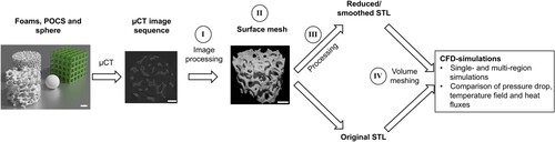
The workflow applied in this work contains an intermediate step of surface reconstruction, it is thus an indirect method. The main reason is a better control over every process step and the broad availability of the required algorithms in available software. Beyond that, existing CFD software like OpenFOAM® (Weller et al., 1998) and STAR-CCM+ (Siemens PLM, Plano, Texas, USA) use STL files as the basis for creating volume meshes. The overall process steps are shown in Figure 2. After µCT (micro-computed tomography) scanning, the voxel-based data is available as an image sequence. These images are processed (ImageJ), the surface is reconstructed, and an STL file is generated (ParaView). The resulting STL file is further processed by decimating the data and smoothing the surface (Blender). For the comparative geometries with known surface and volume (sphere and Periodic Open Cell Structure/POCS), the final STL files are assessed regarding volume and surface fidelity. For the 10 ppi OCF, volume meshes are generated and CFD-simulations are performed to examine the influence of surface mesh smoothing on the volume mesh generation and CFD results.

Figure 2. Schematic of the workflow from the physical object to the final volume mesh. The investigated objects are a sphere, a POCS and a 10 and 20 ppi OCF. The surface mesh represents the geometry, which is the basis for volume mesh generation. The process steps are performed with ImageJ (I), ParaView (II), Blender (III) and OpenFOAM (IV). All scale bars represent 5 mm.

3.2. Geometries and µCT scanning

Apart from a 10 and 20 ppi OCF, we investigate a simple sphere geometry as well as a POCS with known surface and volume to assess the fidelity of the geometrical parameters. The POCS has a cubic unit cell and is generated using the script-based, open-source software OpenSCAD (openscad.org). Both strut diameter and unit cell height are comparable to the values of the 10 ppi OCF. Afterwards, the POCS is 3D printed using an ELEGOO® Mars UV photocuring printer (Shenzhen, China) with an x-y resolution of 47 µm and a z-axis accuracy of 1.25 µm. The photopolymer resin used is the ELEGOO LCD UV 405 nm rapid resin. The open cell foams (manufactured by Hofman Ceramics GmbH, Breitscheid, Germany) as well as the sphere are made from alumina. A standard calliper is used to measure the diameter and height of the samples. The sphere has a diameter of 12.04 mm. The OCFs have a diameter of 25 mm and a height of 22 mm. The geometrical parameters of the objects are summarized in Table 1.

Table 1. Morphological properties of the investigatedgeometries.

	Sphere	POCS	OCF (10 ppi)	OCF (20 ppi)
Total diameter/length [mm]	12.04^a	25^a	25^a	25^a
Open porosity [−]		0.82^b	0.77^b	0.78^b
Specific surface area [m^−1]		514^b	714^b	1369^b
Cell diameter/length [mm]		5	5.76 ± 1.9^c	3.41 ± 0.6^d
Window diameter [mm]			3.3 ± 0.9^c	1.9 ± 0.3^d
Strut diameter [mm]		1.5	1.5 ± 0.5^c	0.87 ± 0.13^e

^a Measured with calliper.

^b Obtained from surface meshes.

^c Sinn et al., 2020.

^d Sadeghi et al., 2020.

^e Calculated with literature correlation (Inayat et al., 2011).

High-resolution X-ray tomography is used to generate digital representations of the examined geometries (X-ray source: XS160NFOF, GE Sensing & Inspection Technologies, USA; detector: Shad-o-Box  6 K HS, Teledyne DALSA, Canada). All scans are performed at TU Dresden using a molybdenum target. The acceleration voltage is set to 90 kV and the cathode current to 170 µA with an exposure time of 0.18 s for the POCS and 1-1.1 s for the other geometries. The angular resolution of 0.25° results in 1440 radiograms per sample. The geometric magnification is 6.05 for the sphere sample, 3.05 for the OCF geometries, and 2.05 for the POCS. The resulting voxel size of the reconstructed data is 8.18 µm for the sphere, 16.23 µm for the foams and 24.15 µm for the POCS. Compared to a minimum resolution of 10 voxels per sphere radius reported in literature (Nyström et al., 2002), the resolutions of the datasets used here are more than sufficient with a minimum of 31 voxels per strut radius for the POCS.

3.3. Post-processing and surface mesh

A standard operating procedure for the process steps can be found in the Supplementary Materials. The workflow from µCT images to the processed surface mesh can be divided into three main steps:

1. Post-processing of image stacks in ImageJ (median filter, binning, and binarisation),

2. surface reconstruction and STL generation in ParaView (Contour filter), and

3. file size reduction and surface smoothing in Blender (decimate collapse algorithm, simple smoothing algorithm).

These steps are performed consecutively. To generate an STL file out of the CT data, the binarisation in step I and the surface reconstruction in step II are the only mandatory steps. The other optional steps help to reduce the file size and improve the surface fidelity of the objects. In the following, we describe the process steps in more detail.

3.3.1. ImageJ

The post processing of the CT data (step I) is done using the open-source software ImageJ Fiji (https://imagej.net/software/fiji/). Firstly, the image stacks are cropped to fit the region of interest and a median filter (radius 3 px) is applied. This helps to get rid of artifacts and noise in the images and is beneficial for the upcoming edge detection (Bovik et al., 1987; Reddy et al., 2017). Thereafter, the images are binned with a value of 0.5 in every 3 directions, so that only half of the pixels are left in each direction. Consequently, the voxel size is doubled and the data is reduced significantly (factor 1/8). This is an optional step and reduces both the file size as well as the resolution of the data. However, in the case of the OCFs binning is necessary to be able to process the data further. For the sphere and the POCS, both the binned and the original image stacks are used from now on to be able to analyse the differences of the resulting STL files. To reconstruct the surface, object and background pixels are identified and separated by applying the default auto-threshold in ImageJ on the grey values of the images. This algorithm is based on the iterative procedure published by Ridler and Calvard (1978), considering the average values of the background and object pixels and setting the threshold to the arithmetic mean of these values in every iteration. After thresholding, the images are segmented and the pixel values are normalized by the object value to get a pseudo-binary image stack (only values of 0 and 1).

3.3.2. ParaView

This image stack is loaded into ParaView (paraview.org) for surface reconstruction (step II). The contour filter is used to create an iso-surface representing the surface of the objects. This filter is part of the Visualization Toolkit (VTK) library (Kitware Inc., Clifton Park, New York, USA). It detects points with a certain value (in this case 0.5) within the interpolated data set and connects them to form a triangulated surface. This surface can directly be exported as an STL file. This approach is trivial but also very efficient, since the outcome is almost identical to the one of the MC algorithm. This is because the MC algorithm also uses linear interpolation. MC is a divide-and-conquer approach creating cells (marching cubes), that are bounded by the centers of 8 pixels of two adjacent slices (Lorensen & Cline, 1987). After finding the cells at the borders, linear interpolation is used to approximate the intersection points of the marching cubes with the iso-surface (Lindblad & Nyström, 2002; Lorensen & Cline, 1987). In this work, the interpolated binary values of each slice are used for surface reconstruction, resulting in a similar surface appearance.

3.3.3. Blender

In step III the mesh is decimated and smoothed. The size of the STL file can be huge, depending on the complexity of the geometry and the resolution of the CT scan (in our case between 250 MB for the binned sphere sample and 12.3 GB for the original 20 ppi OCF if saved as binary files). Such large files cause several problems. Firstly, it costs time since the computational time of the volume mesh increases with file size. Secondly, considerable hardware resources (especially RAM) are required to process this data further (and also to generate volume meshes, see Section 4.2). Further processing is required to tackle problems like non-manifold edges or unconnected vertices, which can result from faulty CT scans. The data is thus reduced using the open-source software Blender® (blender.org). The built-in decimate modifier is used in collapse mode with a factor of 0.1, so that only 10% of the file size is retained. The decimation with the chosen factor of 0.1 does influence the shape of the geometries, which is shown exemplary for the 10 ppi OCF in the Supplementary Materials (Section S1.2). The decimate modifier uses an iterative edge contraction algorithm based on quadric error metrics, comparable to the one proposed by Garland and Heckbert (Garland & Heckbert, 1997; Garland & Heckbert, 1998). In contrast to binning (step I), decimation reduces the file size while preserving the shape of the geometry as much as possible. Therefore, only little geometrical information is lost. A more detailed description of the decimate algorithm can be found in the Supplementary Materials (Section S1.1).

As a last processing step for the surface mesh, smoothing is performed to correct the stepped surface representation. For this, the smooth modifier in Blender was used. The algorithm is very simple and based on averaging of edge center points (detailed description in Supplementary Materials, Section S1.1). In this work, two iterations and a factor of 1 are used, since results show good agreement with the real surface (Section 4.1).

3.4. Volume mesh

The STL files can serve as the basis for the volume mesh generation using a variety of meshing and/or simulation software. This is step IV of the presented workflow. Here, only the reconstructed surface of the 10 ppi OCF is used for volume meshing and simulation. Its complex structure serves as a model for porous geometries, which are often used in engineering applications nowadays. Both single- as well as multi-region meshes are generated to be able to evaluate the performance of different STL files for both cases.

The mesh generator snappyHexMesh (sHM) implemented in the software OpenFOAM is used. While most other mesh generators build the mesh from scratch, sHM uses a given mesh and modifies it to fit the geometry. The base mesh is generated using blockMesh, a pure hexahedral mesh generator implemented in OpenFOAM. In a next step, sHM refines the mesh and snaps adjacent vertices on the surface of the STL geometry. This is done based on mesh quality targets that can be set separately (see OpenFOAM cases in Repository). The final mesh is not purely hexahedral due to different refinement levels and resulting tetrahedrons in the transition areas. The meshing is performed on 6 cores of an AMD® Ryzen® 7 2700 processor. A detailed workflow can be found in the Supplementary Materials (Section S6).

3.5. Governing equations and simulation setup

All CFD simulations are performed using OpenFOAM (v6, https://openfoam.org/download/6-source/), which is based on the Finite Volume Method. A single-phase, steady-state, and laminar fluid flow is simulated. Single- and multi-region simulations are performed using rhoSimpleFoam and chtMultiRegionFoam, respectively. For detailed explanations on the assumption of laminar flow and the governing equations in the fluid phase see Section S3 in the Supplementary Materials.

In case of multi-region simulations, a solid phase is considered. This solid phase can solely be described by the energy equation, which facilitates to (3.1) $\frac{\mathrm{\partial }}{\mathrm{\partial }{x}_i}\stackrel{-q_i}{\overbrace{\left(\frac{{\lambda }_s}{c_{p,s}}\frac{\mathrm{\partial }{h}_s}{\mathrm{\partial }{x}_{\text{i}}}\right)}}=0,$(3.1) where $x_i$ are the Cartesian coordinates, $q_i$ denotes the heat transferred through the solid due to conduction, ${\lambda }_s$ is the solid’s thermal conductivity, $c_{p,s}$ the specific heat capacity of the solid and $h_s$ the enthalpy of the solid. The solid is assumed to be mullite. To mimic the heat production during a heterogeneous catalytic reaction, a heat source is introduced at the interface between the OCF and the fluid. This boundary condition is coded manually by using an existing boundary condition and introducing a reference temperature gradient at the baffle between solid and fluid (source code in Repository). The constant temperature gradient leads to a constant heat flux at the baffle. 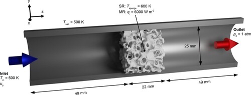The required temperature gradient for a certain heat flux can be calculated using Fourier’s law: (3.2) $\frac{\mathrm{\partial }T}{\mathrm{\partial }{x}_i}=q_i+\lambda$(3.2) with $T$ being the temperature. The value of the heat flux is set to 6000 W·m⁻², leading to a total heat source of about 47 W. This is based on the heat of reaction of the CO₂ methanation, which is estimated to be 44.1 W for a similar OCF by Sinn et al. (2020). A summary of other model assumptions can be found in Table S1 in the Supplementary Materials.

The pressure at all boundaries except at the outlet is considered as zero gradient. A no-slip condition for the velocity is set at the reactor wall as well as the OCF surface. For the single-region simulations, a fixed temperature of 600 K is set at the boundary between fluid and OCF. In case of the multi-region simulations, the surface-based heat source is applied. See Figure 3 for an overview of the simulation area and the boundary conditions.

Figure 3. Overview of the simulation area and the main boundary conditions for single-region (SR) and multi-region (MR) simulations.

4. Results

The Results chapter is divided into three main parts. In the first part, the influence of the process steps on the surface meshes is investigated. These process steps are binning in ImageJ (I), surface reconstruction in ParaView (II), and decimating and smoothing in Blender (III). The surface area and the volume are determined using Blender with exception of the volume of the image stack, which was calculated using the number of solid voxels of the stack. In a second part, the generation of volume meshes for the 10 ppi OCF is examined. By using two different surface meshes (with and without process step III), the differences with regard to required hardware and time for meshing are shown. In a third part, the two generated volume meshes are utilized for CFD simulations to show the influence of surface smoothing on CFD results.

4.1. Surface meshes

4.1.1. Sphere

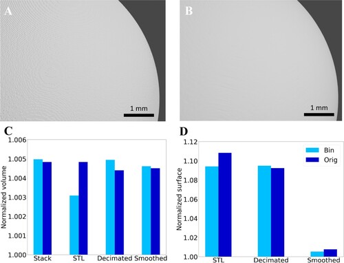
In this section, we compare both volume and surface area of the sphere geometry at specific steps during the presented workflow: the image stack, the surface reconstruction (STL), the surface decimation by quadric error metrics, and the smoothed surface (Figure 4). We further compare the influence of binning for all steps. We did not determine the surface area of the image stack, because the voxel-based data cannot represent the real surface sufficiently (see Chapter 2). The values are normalised with respect to the real values of the sphere, $A=4\pi r^2=4.554\text{ c}{\text{m}}^2$, and $V=\frac{4}{3}\pi r^3=914.08\text{ m}{\text{m}}^3$. The difference between binned and original data is very low for both the surface as well as for the volume (Figure 4(C,D), less than 2% difference between binned and original data during all steps). This shows clearly that the chosen resolution is sufficient to represent the geometry. Thus, binning of the data does not have a significant influence on the geometric parameters. For all the process steps, the volume of the sphere is represented well with a maximum deviation of 0.5%, indicating a high accuracy of the surface reconstruction and STL processing (see Figure 4 C). However, the surface area is significantly overestimated after surface reconstruction (see Figure 4 D). For the binned data, the overestimate is about 9.4%, while for the original data it is 10.8%. This agrees well with the data from Lindblad and Nyström (2002) as well as Nyström et al. (2002), who found an overestimate in surface area for the marching cubes reconstruction of a sphere of about 8.8%. While the decimation does not significantly influence the surface area, it is significantly reduced by the simple smoothing algorithm. After smoothing, the deviation from the real value of the sphere is less than 1%. This surface improvement is visible in Figures 4(A,B). The steps in the surface that cause the overestimate vanish almost completely after smoothing.

Figure 4. Influence of the process steps on the simple sphere geometry (diameter 1.2 cm, material alumina). (A) View onto the surface after surface reconstruction (STL generation). (B) View onto the surface after processing of STL. (C) Volume of the sphere at every consecutive process step normalised by the real value. (D) Surface of the sphere at every consecutive process step normalised with the real values. Dark blue indicates the original (unbinned) data whereas light blue indicates the binned data.

4.1.2. POCS

For the POCS, both volume and the surface are normalised with respect to the digital parent. Similar to the sphere, the process steps do not have a significant influence on the volume of the object (Figure 5(C)). Again, the surface area is overestimated before smoothing (Figure 5(D)). Smoothing once again reduces the surface area by removing the stepped surface (see Figure 5(A,B)). However, the surface after smoothing is lower compared to the digital parent (Figure 5(D)). Furthermore, the volume is overestimated by 3% to 5% (Figure 5(C)).

Figure 5. Influence of the processing steps on the POCS geometry (3D printed). (A) View onto struts after surface reconstruction (STL generation). (B) View onto the struts after processing of the STL. (C) Volume of the POCS at every consecutive process step normalised by the value of the digital parent. (D) Surface of the POCS at every consecutive process step normalised by the value of the digital parent. Dark orange indicates the original (unbinned) data whereas light orange indicates the binned data.

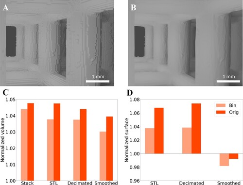
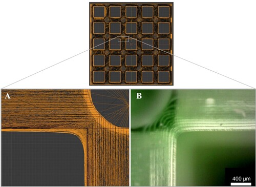
The reason for the underestimation of the surface after smoothing and the overestimation of the volume is rooted in the manufacturing of the POCS. Figure 6(A) shows an orthographic projection of the reconstructed POCS (yellow) superimposed on the digital parent (black). Clearly, the crossing point of the struts is rounded off in the reconstructed POCS leading to a higher volume and lower surface area. This is also seen in the reflected light microscope (Figure 6(B)). The rounding is due to imperfections of the 3D print. We thus still consider smoothing as beneficial to generate a surface appearance closer to reality.

Figure 6. View onto a crossing point of the POCS’ struts. (A) Orthographic projection of the reconstructed POCS (yellow) superimposed on the digital parent (black). (B) Reflected-light microscope image, confirming the manufacturing process causes the differences between reconstructed POCS and digital parent.

4.1.3. OCF

Figure 7 shows, how the process steps are performing on the OCF geometries. Here, the volume is normalised by the value of the image stack and the surface area is normalised with respect to the STL file. This is because the OCFs have a complex structure and hollow struts. This makes it very hard to measure the volume and especially difficult to measure the geometrical surface area experimentally. Additionally, only the binned data is shown here, since data files are very large and no significant impact on the geometrical parameters can be detected.

Still, the process steps do not have a significant influence on the volume (see Figure 7(C)). The maximum deviation is 0.4% for the smoothed 10 ppi sample. Again, the smoothing step leads to a substantial reduction of the surface area, with 12.9% for the 10 ppi and 16.6% for the 20 ppi sample (see Figure 7(D)). Compared to the other geometries, this reduction is considerable. The reason for that is most likely the complex structure of the OCFs with their small cavities inside the struts. This leads to a higher average curvature of the object, so smoothing has a bigger influence on the surface area. The enhancement of the surface representation can be seen in Figure 7(A,B) as well as in the superimposition in Figure 8. Sharp edges and artefacts are reduced, while the overall geometry is maintained.

Figure 7. Influence of the processing steps on the OCF geometry (diameter 2.5 cm). (A) View onto the surface of the 10 ppi OCF after surface reconstruction (STL-generation). (B) View onto the surface of the 10 ppi OCF after processing of STL. (C) Volume of the OCFs at every consecutive process step normalised with the stack values. (D) Surface of the OCFs at every consecutive process step normalised with the STL values. Dark green indicates the 10 ppi OCF whereas light green indicates the 20 ppi OCF. All the data was gained from the binned image stacks.

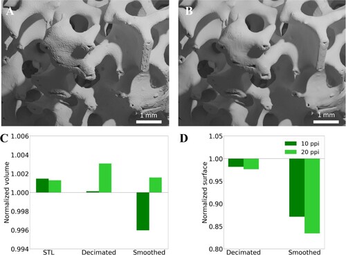
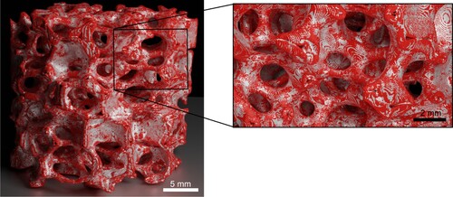
Figure 8. Superimposition of the binned 10 ppi sample without (red, 1.3 GB) and with (white, 130 MB) decimation and smoothing performed. The processing steps reduce the stepped surface appearance while preserving the overall geometry.

Additionally, both the binning and the decimation reduce the data significantly for all samples, as can be seen from Table 2. The original datasets of the OCFs could not be decimated and smoothed as 64 GB of RAM were not enough for further processing. This illustrates the problem of the huge amount of data, which impede the handling of the geometries. However, too much binning can also lead to a loss of the overall geometric structure, if the voxel size increases towards the size of the smallest structures in an object. Hence, it is beneficial to perform most data reduction using the quadric error metrics decimation. In this way, as much geometric details as possible can be used for surface reconstruction and the data reduction is based on an algorithm specifically made to preserve the surface appearance.

Table 2. Required memory size for the individual data files.

	Image		STL decimated/
	stack	STL	smoothed
Sphere orig	13.4 GB	1 GB	103.7 MB
Sphere bin	1.7 GB	256.8 MB	25.7 MB
POCS orig	6.3 GB	1.9 GB	187 MB
POCS bin	792 MB	448 MB	44.8 MB
10 ppi OCF orig	17 GB	5.4 GB	–
10 ppi OCF bin	2.1 GB	1.3 GB	130 MB
20 ppi OCF orig	19.8 GB	12.3 GB	–
20 ppi OCF bin	2.1 GB	2.8 GB	256.2 MB

In conclusion, the performed process steps help to reduce the file size without significantly affecting the volume of the objects. Also, the quadric error metrics-based decimation by a factor of 0.1 does not modify the surface area, indicating the good performance of the algorithm. However, the surface reconstructions lead to an overestimate of the surface areas comparable to reported deviations from the MC algorithm. The simple smoothing algorithm removes the stepped surface appearance leading to a good representation of the surface area. It is clearly shown that it does not make sense using uncompressed data, since the decimated and smoothed meshes show a better representation of the real geometry with less memory space needed.

4.2. Volume meshes

For volume meshing, only the 10 ppi OCF meshes based on the binned, unprocessed STL (1.3 GB, mesh UP) as well as the one based on the processed STL (130 MB, mesh P) are used. The meshing procedure and parameters are identical for the two meshes. Since both single-region and multi-region simulations are performed, both types of volume meshes are generated (see Section S4 in Supplementary Materials for grid independence study).

Figure 9 shows the meshing time as well as the average RAM usage for meshes that reached grid independence. Clearly, both measures are reduced significantly by decimating and smoothing the STL. For the multi-region meshes, the meshing time decreases by more than 45% (Figure 9(A)), while the required RAM decreases by more than 75% (Figure 9(B)). The saved hardware resources are significant. Same results can be seen in case of the single-region mesh. The volume difference between both meshes is below 1% for all of the meshes, in accordance with the surface meshes. When comparing the surface area of the volume-meshed OCF (not shown), the difference between the meshes decreases compared to the surface mesh. The surface of the volume mesh from the unprocessed STL is 2.2% (single-region) and 3.9% (multi-region) larger than the surface of the volume mesh of the processed STL. The volume meshing thus has a smoothing effect on the OCF’s surface, which is due to a larger cell size compared to the resolution of the surface meshes (about 32.46 µm resolution of the binned µCT data compared to 100 µm edge length at the OCF interface in the volume mesh (both single- and multi-region)). However, the surface fidelity of the processed mesh is still better compared to the unprocessed. Although the volume mesh cannot resolve the imperfections of the unprocessed surface mesh, recesses on the OCF surface can be detected. The reason for that is the way the volume mesh is generated. Meshing algorithms try to place or move the nodes of a volume mesh on the projected surface of the surface mesh. If the surface mesh is stepped, defects in the volume mesh are more likely because of the abrupt change of the surface location.

Figure 9. Meshing time (A) and RAM usage (B) for mesh UP and mesh P. Both for single- and multi-region meshes, the smoothed mesh reduces meshing time and RAM usage significantly.

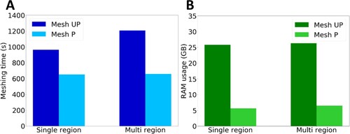
Concluding, processing the STL increases the performance of the volume meshing process significantly. The meshing time is reduced by up to 45% and the average RAM usage decrease from more than 25 GB to about 6 GB. Furthermore, the process of meshing mitigates the overestimation of surface area for the not smoothed STL, having a smoothing effect on the OCF surface.

4.3. Influence on CFD results and the importance of smoothing

In the last section we showed the smoothing caused by the volume meshing. However, differences in the surface area between mesh UP and mesh P are still present, and the surface fidelity is considerably different. In this section we show an application example of the generated volume meshes. It is a proof of feasibility of the generated meshes, but also evaluates the influence of surface-mesh smoothing on CFD results. Since we do not attempt to represent the reality, we do not validate the simulation results with experiments.

4.3.1. Single-region simulations

For the single-region simulations, a fixed temperature of 600 K is set at the boundary between fluid and OCF, emulating a heated OCF with infinite thermal conductivity. Since the temperature of the reactor wall is identical to the inlet temperature of the fluid (500 K), the only heat entering the system is caused by the OCF.

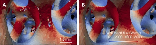
To proof the quality of CFD results, the pressure drop of the OCF for the different velocities is plotted against an analytical correlation in Figure S6 in the Supplementary Materials. The simulated pressure drops are in good agreement with the literature. Comparing mesh UP and mesh P, both flow and temperature fields do not show significant differences, so these results are not discussed here and can be found in the Supplementary Materials as well (Section S5). However, the influence of the poor surface representation of mesh UP on the heat transfer is visible from evaluating the heat flux through the fluid/OCF boundary. Despite a higher volume (+0.8%) and a higher surface area (+2.2%), the integral heat flow of the OCF in mesh UP is 1.28% lower compared to mesh P (values for a superficial velocity of 0.5 m s⁻¹). The reason is clearly seen in Figure 10(A,B). The heat flux is dependent on the temperature gradient near the wall and therefore coupled with the near wall velocity of the fluid. The smoother surface of mesh P leads to a consistent, high velocity gradient near the wall, whereas recesses in the unsmoothed mesh UP cause lower near-wall velocities and thus lower temperature gradients. The consequence is a higher integral heat flow for the smoother mesh.

Figure 10. Single-region simulations. (A) Wall heat flux at a section of the OCF for mesh UP. (B) Wall heat flux at a section of the OCF for mesh P. Heat flux is given in W m⁻² at 0.5 m s⁻¹ inlet velocity.

To conclude, no significant differences between smoothed and unsmoothed meshes could be detected regarding pressure drop as well as regarding local velocity and temperature fields. However, the comparison of the integral heat fluxes showed a 1.28% higher value for mesh P, although both volume and surface area of the OCF are lower compared to mesh UP. The reason for that are recesses in mesh UP, which decrease the local heat flux. The smoothing of the STL thus has a positive influence on the CFD results.

4.3.2. Multi-region simulations

The multi-region meshes are used to perform conjugate heat transfer simulations. For this, a surface-based heat source is added at the interface between fluid and solid region. This is an easy way to mimic the heat production during a heterogeneous, catalytic reaction, assuming a homogeneous heat production dependent on the surface area. In this case, a power of 6000 W·m⁻² is introduced.

A radial averaging method is used to compare radial temperature profiles (similar to Sinn et al., 2020). We chose two slices, located at the front and back of the foam, which we divided into 10 annuli with equal area. The temperature was averaged within these annuli (Figure 11(A)). Hence, a radial temperature profile can be extracted for the fluid and the solid region at two distinct positions at the front and back of the foam. Results for an inlet velocity of 0.3 m s⁻¹ can be seen in Figure 11(B,C). Temperatures are plotted over the normalized radius. The solid temperature is higher than the fluid temperature, because a large part of the heat is introduced into the solid due to its higher thermal conductivity. Also, the temperature is higher towards the back of the OCF, since the fluid heats up downstream effectively reducing the cooling effect of the fluid. The temperature decreases with radius, underlining the strong effect of wall cooling through conduction in the foam struts.

Figure 11. Radial averaging of temperature. (A) Illustration of the temperature analysis method. Two slides are located 3 mm downstream of the beginning (front) and 3 mm upstream of the end of the OCF (back). 10 annuli with equal areas were used to perform a radial averaging of the temperatures. (B) Radial temperature distribution in the front slice for the two different meshes. (C) Radial temperature distribution in the back slice for the two different meshes (evaluation method similar to Sinn et al., 2020).

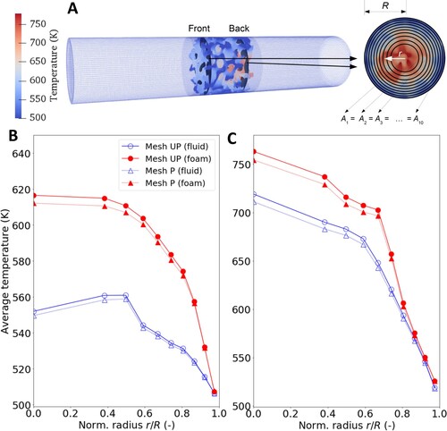
Results from Figure 11 show lower temperatures for the smoothed OCF (mesh P) due to the lower surface area. The radial averaging shows an effect on the temperature distribution especially in the centre of the foam (small r/R), with a maximum difference of 9 K. The difference decreases with increasing r/R because of the high conduction through the struts.

Although the difference between the two meshes seems to be quite low, the influence on simulations with catalytic surface reactions can be of importance. The amount of accessible surface area is of utmost importance for heterogeneous catalytic reactions, since it (together with the catalyst loading) determines the number of active sites. As a result, the overestimated surface area in mesh UP would lead to higher conversion. In exothermic reactions, higher temperatures and additionally accelerated reactions kinetics are the consequences. Thus, small differences in the surface area could have a significant influence on the whole system. Furthermore, the simulation of heterogeneous catalytic reactions is especially dependent on the surface fidelity and near-wall cells. Reactions take place at the interface between solid and fluid and, numerically, the heat of reaction is introduced into the fluid cells at the solid (this is the case for the OpenFOAM add-on DUO, Deutschmann et al., 2020). The resulting high gradients in temperature and species concentration require cells of high quality to guarantee convergence of the simulations and realistic results. Additionally, recesses like the ones we showed for the mesh UP can lead to additional problems, since transport of the reaction heat is limited due to missing convection. This makes complex reaction simulations more prone to errors. The improved discretization based on the smoothed STL is therefore beneficial for sound reactive CFD simulations.

Concluding, the surface-based heat source method shows differences between the smoothed and unsmoothed mesh. Both heat flux and temperature are higher for mesh UP, which is due to the overestimation of the surface area. Considering actual reaction simulations, the influence of the unsmoothed mesh on the results can be even higher, which is why smoothing of the surface mesh is highly desirable.

5. Discussion

The results clearly show the quality of the workflow’s outcome and how both the decimating and smoothing algorithms in Blender are suitable to process the µCT data. While the decimate modifier based on quadric error metrics saves time and resources in volume meshing, the surface smoothing is necessary to preserve the surface area. To our knowledge, this study shows for the first time, how a stepped surface representation of unsmoothed CT reconstructions can have an influence on CFD results. Hence, special care should be taken when processing CT data and the presented workflow can build the basis for that.

The open-source nature gives the opportunity to establish a standardised way to prepare image-based CFD simulations, free to use for everyone. In literature, the reported ways of processing CT data and generating volume meshes for simulations are very diverse and often both fragmentary as well as based on commercial software tools. For surface-mesh generation, the software Mimics (Materialize NV, Belgium) is widely used in biomedical applications (Cherobin et al., 2018; Kou et al., 2018; Qi et al., 2018; Sun et al., 2022), while also in-house segmentation codes are used (Thune et al. 2021). In other disciplines the approaches are more diverse, ranging from commercial software like ScanIP (Della Torre et al., 2014; Yang et al., 2019), Retomo (Aboukhedr et al., 2017), VGStudio Max (Dong et al., 2018), and Octopus (Emmel et al., 2020; developed by Dierick et al., 2004) to open-source software like ImageJ (Emmel et al., 2020; Moreno-Casas et al. 2020; Plachá et al., 2020; Shimotori et al., 2021). Further processing is done in software like SOLIDWORKS (Sun et al., 2022), STAR-CCM+ (Dong et al., 2018; Thune et al., 2021), ANSA (Aboukhedr et al., 2017) and Geomagic Studio (Qi et al., 2018). This diversity in combination with the commercial nature of the used software packages makes it difficult for other scientists to reproduce the data, which is essential to maintain good scientific practice. The presented workflow overcomes these challenges and gives a potential guideline for standardised pre-processing of image-based CFD.

Furthermore, the workflow can easily be extended for special demands. Apart from the influence of surface smoothing on CFD results shown here, the model reconstruction itself also impacts CFD results, as was shown by Cherobin et al. (2018). Different Hounsfield value thresholds can change both the geometry as well as the pressure loss and flow rate in simulated nasal airflow (Cherobin et al., 2018). However, in the present study, using a single-component material the default auto threshold in ImageJ showed a very good outcome in preserving geometrical parameters, which is why there was no need to consider threshold differences. For applications in biomedical engineering with a large number of different tissues to be segmented, the choice of a proper threshold can be of higher importance. Also, in special applications like image-based CFD of cement pores, deconvolution techniques have to be used to make segmentation even possible (Yang et al., 2019). Consequently, the present workflow has to be extended with a special focus on the segmentation of CT data, if special applications are considered.

6. Conclusion

In this work, we introduce an easy-to-use workflow for the processing of CT image sequences into sound volume meshes. This workflow is based on open-source software and the resulting meshes can be directly used for CFD simulations. A detailed description of the workflow including STL data and CFD cases is provided in the Supplementary Materials. The basic steps of the workflow are: [I] Post processing of CT image stack (ImageJ), [II] reconstruction of the surface (ParaView), [III] decimating and smoothing of the surface mesh (Blender), and [IV] volume meshing as a basis for CFD simulations (snappyHexMesh in OpenFOAM). It was possible to decimate the STL size by 90% without having an influence on the surface area or the volume. By using geometries with known volume and surface area, the surface meshes could be evaluated in terms of the preservation of morphological parameters. While the volume was almost consistent throughout all the process steps, the surface area was overestimated by up to 10.8% due to a stepped surface after surface reconstruction. Smoothing of the surface resulted in a better agreement with the real values. In summary, processing of the CT data reduced the files to a large extend and improved the overall surface fidelity. This reduced the volume meshing time by up to 45% and the RAM usage by up to 75%.

Furthermore, CFD simulations were performed to assess the influence of surface smoothing on simulation results. Recesses in the unsmoothed mesh led to poor heat flux representations at the fluid/solid interface. Moreover, used surface heat sources showed higher temperatures in the unsmoothed mesh due to a larger surface area. Hence, smoothing of surface reconstructions is advisable and can be of high importance, if the surface area or the quality of near-wall cells is especially important (e.g. in the case of catalytic surface reactions).

Finally, we discuss the findings and the workflow itself by comparing it with recent literature in the field of image-based CFD. By now, a wide range of (often commercial) software is used, which makes it difficult to reproduce data. Our workflow offers the opportunity to overcome this challenge, since it relies only on open-source software. While the application for single component materials is our main focus, the workflow can easily be extended for special application, where the choice of a proper threshold during segmentation is of higher importance.

In summary, we showed that processing CT data with open-source software can save both time as well as resources and deliver high quality meshes for consecutive CFD simulations. The provided standardised workflow facilitates the work for engineers in the field of image-based CFD and is not limited to the presented cases of foams or POCS.

Acknowledgements

The authors thank Prof. Dr. Stefan Odenbach, head of the Chair of Magnetofluiddynamics, Measurement and Automation Technology at the TU Dresden, for providing the resources and equipment necessary for performing the µCT scans. Moreover, we thank Thomas Ilzig, also from TU Dresden, for assistance regarding the µCT scans. Kevin Kuhlmann wants to thank Christoph Kühn from the group of Thermofluid Dynamics at the Center of Applied Space Technology and Microgravity (ZARM, Uni Bremen) for his helpful assistance with coding of the surface heat source in OpenFOAM. Furthermore, Kevin Kuhlmann thanks Prof. Dr. Rodion Groll, head of the group of Thermofluid Dynamics at ZARM (Uni Bremen), for helpful discussions regarding this manuscript and assistance in numerical and fluid dynamic questions.

Data deposition

All data relevant to this work and detailed explanations are available under https://doi.org/10.5281/zenodo.6521710.

Disclosure statement

No potential conflict of interest was reported by the author(s).

Additional information

Funding

This work was supported by the German Research Foundation (DFG) through the research training group GRK 1860 (Micro-, Meso- and Macroporous Nonmetallic Materials: Fundamentals and Applications, MIMENIMA).

References

- Aboukhedr, M., Mitroglou, N., Georgoulas, A., Marengo, M., & Vogiatzaki, K.. (2017). Simulation of droplet spreading on micro-CT reconstructed 3D real porous media using the volume-of-fluid method. Ilass Europe. 28th european conference on Liquid Atomization and Spray Systems, Valencia, Spain. https://doi.org/10.4995/ILASS2017.2017.4755 .
- Agostini, E., Boccardo, G., & Marchisio, D. (2022). An open-source workflow for open-cell foams modelling: Geometry generation and CFD simulations for momentum and mass transport. Chemical Engineering Science, 255, 117583. https://doi.org/10.1016/j.ces.2022.117583.
- Ali, Z., Tyacke, J., Watson, R., Tucker, P. G., & Shahpar, S. (2019). Efficient preprocessing of complex geometries for CFD simulations. International Journal of Computational Fluid Dynamics, 33(3), 98–114. https://doi.org/10.1080/10618562.2019.1606421
- Bovik, A. C., Huang, T. S., & Munson, D. C. (1987). The effect of median filtering on edge estimation and detection. IEEE Transactions on Pattern Analysis and Machine Intelligence, 2(2), 181–194. https://doi.org/10.1109/TPAMI.1987.4767-894
- Cherobin, G. B., Voegels, R. L., Gebrim, E. M., & Garcia, G. J. (2018). Sensitivity of nasal airflow variables computed via computational fluid dynamics to the computed tomography segmentation threshold. PLoS One, 13(11), e0207178. https://doi.org/10.1371/journal.pone.0207178
- Della Torre, A., Montenegro, G., Tabor, G. R., & Wears, M. L. (2014). CFD characterization of flow regimes inside open cell foam substrates. International Journal of Heat and Fluid Flow, 50, 72–82. https://doi.org/10.1016/j.ijheatfluidflow.2014.05.005
- Deutschmann, O., Tischer, S., Correa, C., Chatterjee, D., Kleditzsch, S., Janardhanan, V. M., Mladenov, N., Minh, H. D., Karadeniz, H., Hettel, M., Menon, V., Banerjee, A., Goßler, H., Daymo, E. (2020) DETCHEM Software package, 2.8 ed. www.detchem.com.
- Dierick, M., Masschaele, B., & Van Hoorebeke, L. (2004). Octopus, a fast and user-friendly tomographic reconstruction package developed in LabView®. Measurement Science and Technology, 15(7), 1366–1370. https://doi.org/10.1088/0957-0233/15/7/020.
- Dong, Y., Korup, O., Gerdts, J., Cuenya, B. R., & Horn, R. (2018). Microtomography-based CFD modeling of a fixed-bed reactor with an open-cell foam monolith and experimental verification by reactor profile measurements. Chemical Engineering Journal, 353, 176–188. https://doi.org/10.1016/j.cej.2018.07.075
- Emmel, D., Hofmann, J. D., Arlt, T., Manke, I., Wehinger, G. D., & Schröder, D. (2020). Understanding the impact of compression on the active area of carbon felt electrodes for redox flow batteries. ACS Applied Energy Materials, 3(5), 4384–4393. https://doi.org/10.1021/acsaem.0c00075
- Garland, M., & Heckbert, P. S.. (1997). Surface simplification using quadric error metrics. Proceedings of the 24th annual conference on computer graphics and interactive techniques. https://doi.org/10.1145/258734.258849.
- Garland, M., & Heckbert, P. S.. (1998). Simplifying surfaces with color and texture using quadric error metrics. VIS '98: Proceedings of the conference on Visualization '98. https://doi.org/10.1109/VISUAL.1998.745312.
- Grove, O., Rajab, K., Piegl, L. A., & Lai-Yuen, S. (2011). From CT to NURBS: Contour fitting with B-spline curves. Computer-Aided Design and Applications, 8(1), 3–21. https://doi.org/10.3722/cadaps.2011.3-21
- Inayat, A., Freund, H., Zeiser, T., & Schwieger, W. (2011). Determining the specific surface area of ceramic foams: The tetrakaidecahedra model revisited. Chemical Engineering Science, 66(6), 1179–1188. https://doi.org/10.1016/j.ces.2010.12.031
- Inthavong, K., Wen, J., Tu, J., & Tian, Z. (2009). From CT scans to CFD modelling–fluid and heat transfer in a realistic human nasal cavity. Engineering Applications of Computational Fluid Mechanics, 3(3), 321–335. https://doi.org/10.1080/19942060.2009.11015274
- Kagadis, G. C., Skouras, E. D., Bourantas, G. C., Paraskeva, C. A., Katsanos, K., Karnabatidis, D., & Nikiforidis, G. C. (2008). Computational representation and hemodynamic characterization of in vivo acquired severe stenotic renal artery geometries using turbulence modeling. Medical Engineering & Physics, 30(5), 647–660. https://doi.org/10.1016/j.medengphy.2007.07.005
- Kou, G., Li, X., Wang, Y., Lin, M., Zeng, Y., Yang, X., Yang, Y., & Gan, Z. (2018). CFD simulation of airflow dynamics during cough based on CT-scanned respiratory airway geometries. Symmetry, 10(11), 595. https://doi.org/10.3390/sym10110595.
- Krajnovic, S., & Davidson, L. (2000). Flow around a three-dimensional bluff body. In 9th international symposium on flow visualization, Heriot-Watt Univeristy, Edinburgh.
- Lindblad, J., & Nyström, I.. (2002). Surface Area Estimation of Digitized 3D Objects Using Local Computations . DGCI 2002: International Conference on Discrete Geometry for Computer Imagery, Bordeaux, France. https://doi.org/10.1007/3-540-45986-3_24.
- Lintermann, A. (2021). Computational meshing for CFD simulations. In Kiao Inthavong, Narinder Singh, Eugene Wong, & Jiyuan Tu (Eds.), Clinical and biomedical engineering in the human nose (pp. 85–115). Springer Singapore.
- Lorensen, W. E., & Cline, H. E. (1987). Marching cubes: A high resolution 3D surface construction algorithm. ACM Siggraph Computer Graphics, 21(4), 163–169. https://doi.org/10.1145/37402.37422
- Manmadhachary, A., Kumar, R., & Krishnanand, L. (2016). Improve the accuracy, surface smoothing and material adaption in STL file for RP medical models. Journal of Manufacturing Processes, 21, 46–55. https://doi.org/10.1016/j.jmapro.2015.11.006
- Meinicke, S., Möller, C. O., Dietrich, B., Schlüter, M., & Wetzel, T. (2017a). Experimental and numerical investigation of single-phase hydrodynamics in glass sponges by means of combined µPIV measurements and CFD simulation. Chemical Engineering Science, 160, 131–143. https://doi.org/10.1016/j.ces.2016.11.027
- Meinicke, S., Wetzel, T., & Dietrich, B. (2017b). Scale-resolved CFD modelling of single-phase hydrodynamics and conjugate heat transfer in solid sponges. International Journal of Heat and Mass Transfer, 108, 1207–1219. https://doi.org/10.1016/j.ijheatmasstransfer.2016.12.052
- Menegazzi, P., & Trapy, J. (1997). A new approach to the modelling of engine cooling systems. Revue de l'Institut Français du Pétrole, 52(5), 531–539. https://doi.org/10.2516/ogst:1997058
- Moreno-Casas, P. A., Scott, F., Delpiano, J., & Vergara-Fernández, A. (2020). Computational tomography and CFD simulation of a biofilter treating a toluene, formaldehyde and benzo [α] pyrene vapor mixture. Chemosphere, 240, Article 124924. https://doi.org/10.1016/j.chemosphere.2019.124924
- Müller, R., & Rüegsegger, P. (1995). Three-dimensional finite element modelling of non-invasively assessed trabecular bone structures. Medical Engineering & Physics, 17(2), 126–133. https://doi.org/10.1016/1350-4533(95)91884-J
- Nowak, N., Kakade, P. P., & Annapragada, A. V. (2003). Computational fluid dynamics simulation of airflow and aerosol deposition in human lungs. Annals of Biomedical Engineering, 31(4), 374–390. https://doi.org/10.1114/1.1560632
- Nyström, I., Udupa, J. K., Grevera, G. J., & Hirsch, B. E.. (2002). Area of and volume enclosed by digital and triangulated surfaces . Proceedings Volume 4681, Medical Imaging 2002: Visualization, Image-Guided Procedures, and Display, San Diego, California, USA.https://doi.org/10.1117/12.466977.
- Plachá, M., Kočí, P., Isoz, M., Svoboda, M., Price, E., Thompsett, D., Kallis K., & Tsolakis, A. (2020). Pore-scale filtration model for coated catalytic filters in automotive exhaust gas aftertreatment. Chemical Engineering Science, 226, Article 115854. https://doi.org/10.1016/j.ces.2020.115854
- Qi, S., Zhang, B., Yue, Y., Shen, J., Teng, Y., Qian, W., & Wu, J. (2018). Airflow in tracheobronchial tree of subjects with tracheal bronchus simulated using CT image based models and CFD method. Journal of Medical Systems, 42(4), 1–15. https://doi.org/10.1080/10255842.2018.1522531
- Qiu, Y., Yuan, D., Wang, Y., Wen, J., & Zheng, T. (2018). Hemodynamic investigation of a patient-specific abdominal aortic aneurysm with iliac artery tortuosity. Computer Methods in Biomechanics and Biomedical Engineering, 21(16), 824–833. https://doi.org/10.1080/10255842.2018.1522531
- Quadrio, M., Pipolo, C., Corti, S., Messina, F., Pesci, C., Saibene, A. M., Zampini S., & Felisati, G. (2016). Effects of CT resolution and radiodensity threshold on the CFD evaluation of nasal airflow. Medical & Biological Engineering & Computing, 54(2-3), 411–419. https://doi.org/10.1007/s11517-015-1325-4
- Reddy, R. V. K., Raju, K. P., Kumar, M. J., Kumar, L. R., Prakash, P. R., & Kumar, S. S. (2017). Comparative analysis of common edge detection algorithms using pre-processing technique. International Journal of Electrical and Computer Engineering, 7(5), 2574–2580. https://doi.org/10.11591/ijece.v7i5.pp2574-2580
- Ridler, T. W., & Calvard, S. (1978). Picture thresholding using an iterative selection method. IEEE Transactions on Systems, Man, and Cybernetics, 8(8), 630–632. https://doi.org/10.1109/TSMC.1978.4310039
- Rychlik, M., Morzyński, M., Nowak, M., Stankiewicz, W., Łodygowski, T., & Ogurkowska, M. B. (2004). Acquisition and transformation of biomedical objects to CAD systems. Strojnicky Casopis, 55(3), 121–135.
- Sadeghi, M., Mirdrikvand, M., Pesch, G. R., Dreher, W., & Thöming, J. (2020). Full-field analysis of gas flow within open-cell foams: Comparison of micro-computed tomography-based CFD simulations with experimental magnetic resonance flow mapping data. Experiments in Fluids, 61(5), 1–16. https://doi.org/10.1007/s00348-020-02960-4
- Shimotori, S., Kaneko, T., Yoshimoto, Y., Kinefuchi, I., Alizadeh, A., Hsu, W. L., & Daiguji, H. (2021). Evaluation of gas permeability in porous separators for polymer electrolyte fuel cells: Computational fluid dynamics simulation based on micro-x-ray computed tomography images. Physical Review E, 104(4), Article 045105. https://doi.org/10.1103/PhysRevE.104.045105
- Shukla, R. K., Srivastav, V. K., Paul, A. R., & Jain, A. (2020). Fluid structure interaction studies of human airways. Sādhanā, 45(1), 1–6. https://doi.org/10.1007/s12046-020-01460-9
- Sinn, C., Kranz, F., Wentrup, J., Thöming, J., Wehinger, G. D., & Pesch, G. R. (2020). CFD simulations of radiative heat transport in open-cell foam catalytic reactors. Catalysts, 10(6), 716. https://doi.org/10.3390/catal10060716.
- Sinn, C., Pesch, G. R., Thöming, J., & Kiewidt, L. (2019). Coupled conjugate heat transfer and heat production in open-cell ceramic foams investigated using CFD. International Journal of Heat and Mass Transfer, 139, 600–612. https://doi.org/10.1016/j.ijheatmasstransfer.2019.05.042
- Sun, H. T., Sze, K. Y., Chow, K. W., & On Tsang, A. C. (2022). A comparative study on computational fluid dynamic, fluid-structure interaction and static structural analyses of cerebral aneurysm. Engineering Applications of Computational Fluid Mechanics, 16(1), 262–278. https://doi.org/10.1080/19942060.2021.2013322
- Tabe, R., Rafee, R., Valipour, M. S., & Ahmadi, G. (2021). Investigation of airflow at different activity conditions in a realistic model of human upper respiratory tract. Computer Methods in Biomechanics and Biomedical Engineering, 24(2), 173–187. https://doi.org/10.1080/10255842.2020.1819256
- Tabor, G., Yeo, O., Young, P., & Laity, P. (2008). CFD simulation of flow through an open cell foam. International Journal of Modern Physics C, 19(05), 703–715. https://doi.org/10.1142/S0129183108012509
- Tasciyan, T. A., Banerjee, R., Cho, Y. I., & Kim, R. (1993). Two-dimensional pulsatile hemodynamic analysis in the magnetic resonance angiography interpretation of a stenosed carotid arterial bifurcation. Medical Physics, 20(4), 1059–1070. https://doi.org/10.1118/1.597002
- Thune, E. L., Kosinski, P., Balakin, B. V., & Alyaev, S. (2021). A numerical study of flow field and particle deposition in nasal channels with deviant geometry. Engineering Applications of Computational Fluid Mechanics, 15(1), 180–193. https://doi.org/10.1080/19942060.2020.1863267
- Tippe, A., Perzl, M., Li, W., & Schulz, H. (1999). Experimental analysis of flow calculations based on HRCT imaging of individual bifurcations. Respiration Physiology, 117(2-3), 181–191. https://doi.org/10.1016/S0034-5687(99)00052-3
- Wang, C. S., Wang, W. H. A., & Lin, M. C. (2010). STL rapid prototyping bio-CAD model for CT medical image segmentation. Computers in Industry, 61(3), 187–197. https://doi.org/10.1016/j.compind.2009.09.005
- Wehinger, G. D., Heitmann, H., & Kraume, M. (2016). An artificial structure modeler for 3D CFD simulations of catalytic foams. Chemical Engineering Journal, 284, 543–556. https://doi.org/10.1016/j.cej.2015.09.014
- Weller, H. G., Tabor, G., Jasak, H., & Fureby, C. (1998). A tensorial approach to computational continuum mechanics using object-oriented techniques. Computers in Physics, 12(6), 620–631. https://doi.org/10.1063/1.168744
- Wood, B. D., He, X., & Apte, S. V. (2020). Modeling turbulent flows in porous media. Annual Review of Fluid Mechanics, 52(1), 171–203. https://doi.org/10.1146/annurev-fluid-010719-060317
- Yang, X., Kuru, E., Gingras, M., & Iremonger, S. (2019). CT-CFD integrated investigation into porosity and permeability of neat early-age well cement at downhole condition. Construction and Building Materials, 205, 73–86. https://doi.org/10.1016/j.conbuildmat.2019.02.004
- Yoo, D. J. (2011). Three-dimensional human body model reconstruction and manufacturing from CT medical image data using a heterogeneous implicit solid based approach. International Journal of Precision Engineering and Manufacturing, 12(2), 293–301. https://doi.org/10.1007/s12541-011-0039-2
- Young, P. G., Beresford-West, T. B. H., Coward, S. R. L., Notarberardino, B., Walker, B., & Abdul-Aziz, A. (2008). An efficient approach to converting three-dimensional image data into highly accurate computational models. Philosophical Transactions of the Royal Society A: Mathematical, Physical and Engineering Sciences, 366(1878), 3155–3173. https://doi.org/10.1098/rsta.2008.0090