CFD-aided study on transient wave-blockage interaction in a pressurized fluid pipeline

Abstract

Blockages are commonly formed in fluid pipelines such as water supply systems, which may greatly affect the internal flow states and conveyance capacities. This paper investigates the transient behavior of a pressured water pipeline with blockage under different transient wave perturbations based on the Computational Fluid Dynamics (CFD) model. To this end, a water pipeline is modeled in a 2D axisymmetric geometry with refined mesh and the blockage is modeled as a small, constricted section. Both the low and high-frequency waves (LFW and HFW), in terms of radial fundamental wave frequency of a pipeline, ∼a/R, with a being acoustic wave speed and R being pipe radius, are injected for the numerical analysis. Through this CFD model, both the axial and radial transient waves have been observed for different frequency wave injections, which are firstly validated by datasets available from former studies. After validations, the local flow characteristics, such as the velocity field, the vorticity field, and its temporal, spatial evolution in the vicinity of blockage during transient wave processes, including before and after transient wavefront passing, are elaborated and analysed in this study. The results indicate the significant influence of blockages on transient behaviors, especially under high-frequency wave conditions.

KEYWORDS:

• Blockage
• high-frequency wave (HFW)
• low-frequency wave (LFW)
• transient pipe flow
• CFD

1. Introduction

Blockages, such as the buildup and scale-up of the material in the inner pipe wall due to complex physical or chemical processes (Chahardah-Cherik et al., 2021; Duan et al., 2012; Keramat & Zanganeh, 2019; Liu et al., 2017; Louati et al., 2017; Zhao et al., 2018) or flow disturbance caused by partially closed valves (Ferreira et al., 2018; Jewell & Denier, 2013; Meniconi et al., 2012, 2014) and other connected hydraulic devices (Contractor, 1965; Stephens et al., 2007), commonly exist in urban water supply pipelines (UWSP). These faults can not only increase additional energy transmission costs (Duan et al., 2012) but also produce potential risks of water leakage due to complex flow and pressure variations in the vicinity of these faults under steady and unsteady flow states (transient waves) in the system (Duan et al., 2020; Zhao et al., 2018). However, limited by relatively little available external visible or acoustic information offered by blockages under steady-state flow conditions (Zouari et al., 2019), transient-based methods (TBMs), have been developed as one of the intentional detection techniques for pipeline blockages with higher efficiency and accuracy (Lee et al., 2008). The fundamental of the TBMs for blockage detection procedure is based on a modification of the blockage on the transient waveforms (Chaudhry, 2014; Duan et al., 2014; Lee et al., 2008; Meniconi et al., 2014; Zouari et al., 2019). Therefore, to ensure the accuracy and the rationality of the detection result, it is particularly important to have an in-depth understanding of physically modeling the blockage and its interaction with transient waves forwardly (Duan, 2016; Che et al., 2021).

Realistic partial blockages commonly have a certain longitudinal length with a varying cross-sectional area shape. These blockages could be primarily classified into two categories based on their relative length compared with the thickness of the probing wave (Duan et al., 2020; Zhao et al., 2018): (i) discrete blockage or localized (i.e. which is considered as a localized discontinuity); (ii) extended blockage. For the analytical modeling of the discrete blockage in transients, it is assumed that the discharge conservation keeps while additional pressure head loss occurs before and after the blockage (Chaudhry, 2014; Kim, 2018; Lee et al., 2008). Under this assumption, only the blockage location and severity (i.e. blockage-induced local head loss) are unknown based on the measured transient pressure signals for detection. In comparison, one additional area function A(x) that describes the blockage shape for the extended blockage is required to be reconstructed. Specifically, A(x) = constant if the real extended blockage is simplified as a uniform constriction along the pipe axis (Chaudhry, 2014; Duan et al., 2014), and A(x) = a function of x if the effect of its nonuniformity on the system’s transient behavior is so large that cannot be neglected (Che et al., 2018a, 2019; Yan et al., 2021; Zouari et al., 2019).

It is noticed that the majority of these analytical and numerical investigations of transient behaviors in a pipeline with blockage in the time domain or frequency domain are commonly based on the one-dimensional (1D) water hammer equations due to their computational efficiency and convenience for implementation. As a result, the detailed flow dynamics and interactions of transient waves with such blockage cannot be well represented and interpreted from the current 1D models and methods, which is the main content of this study. For clarity, the scope of this study is mainly confined to the rigid pipeline (e.g. with elastic/metallic pipe materials), while for viscoelastic/plastic pipes (e.g. PE or PVC), the effect of pipe wall deformation may induce potential influence on transient wave behavoirs and energy transformation process (Duan et al., 2010; Pan et al., 2020, 2021), which is not considered in this paper.

The computational fluid dynamics (CFD) approach succeeds in many aspects of hydraulic transient numerical simulations with high reliability: (i) the movement of an entrapped air pocket in a water-filling pipe (Zhou et al., 2011); (ii) the atomization process of air and water in a dual-fluid atomizer (Yu et al., 2019); (iii) driving forces in a geyser event (Shao & Yost, 2018); (iv) dynamic characteristics of a closing ball valve (Cao et al., 2022); (v) transient flow characteristics in a reservoir-pipeline-valve (RPV) system with an intact pipe (Martins et al., 2014, 2016, 2018; Wang et al., 2017); and (vi) transient flow characteristics in a RPV system with defects, such as leaks (Lai et al., 2021), and an extended bottom blockage (Zhao et al., 2018). In the aforementioned literature most related to this work (e.g. listed in (v)), we notice that some studies are based on the 2D CFD model (Martins et al., 2018) while others are based on the 3D CFD model (Martins et al., 2014, 2016; Wang et al., 2017), both types get good agreement with the results shown 1D model in predicting the area-averaged transient pressure and the exact or semi-empirical solutions in predicting the velocity profile. However, relative coarse mesh schemes in these studies lead to a deficiency in observing the radial wave behavoirs. Therefore, considering the computational cost, this study finally chooses the 2D CFD model with fine mesh schemes to investigate the 2D transient behavior of a water supply pipeline with a discrete blockage under different wave perturbations for transient generations via the CFD software, Ansys Fluent 18.1. Inspired by the work from (Che et al., 2018a), in which radial pressure wave behavior in an intact pipe and its generation mechanism under different transient operations are well explained, this study investigates how blockage interacts with different frequency wave injections and the local flow characteristics in the vicinity of blockage.

2. Problem description and modeling

2.1. Problem description

The wave propagation in a RPV system with a single discrete blockage is investigated in a fully 2D framework. In the computation domain, the discrete blockage is modeled as a uniform constricted pipe section which means the whole pipe is modeled as an axisymmetric cylindrical configuration (see Figure 1). The dimensionless length of this blockage l_b/L = 8e-5 is minor compared with the thickness of the probing wave. The centroid of the blockage is located as x_b/L = 0.5 while its severity is characterized by its dimensionless radius r_b/R = 0.5. The upstream end of the pipe is bounded by a constant level reservoir with pressure head H_res= 40 m and the downstream is bounded by a valve which is a transient source that produces transient pressure waves (Kim, 2022) with a plane wave speed a. Specific system information and initial flow parameters are listed in Table 1.

Figure 1. Configuration of pipeline with discrete blockage in axial cross-sectional view.

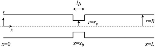
Table 1. System parameters of the CFD numerical experiment.

Hres (m)	L (m)	R (m)	Re	a (m/s)	Tth (s)	fr (Hz)	lb/L	rb/R	xb/L
40	10	0.02	800	1485	0.0269	74250	8e-5	0.5	0.5

2.2. Modeling and numerical schemes

Mathematical models

The full-2D water hammer model, in the cylindrical coordinates, is composed of a continuity equation and momentum equation (Che, 2019; Mitra & Rouleau, 1985): (1) $\begin{array}{rl}& \frac{\mathrm{\partial }p}{\mathrm{\partial }t}+u\frac{\mathrm{\partial }p}{\mathrm{\partial }x}+v\frac{\mathrm{\partial }p}{\mathrm{\partial }r}+K\left(\frac{\mathrm{\partial }u}{\mathrm{\partial }x}+\frac{1}{r}\frac{\mathrm{\partial }(rv)}{\mathrm{\partial }r}\right)=0\end{array}$(1) (2) $\begin{array}{rl}& \frac{\mathrm{\partial }u}{\mathrm{\partial }t}+u\frac{\mathrm{\partial }u}{\mathrm{\partial }x}+v\frac{\mathrm{\partial }u}{\mathrm{\partial }r}\\ & =-\frac{1}{{\rho }_0}\frac{\mathrm{\partial }p}{\mathrm{\partial }x}+\frac{\mu }{{\rho }_0}(\frac{4}{3}\frac{{\mathrm{\partial }}^{2}u}{\mathrm{\partial }{x}^2}+\frac{1}{r}\frac{\mathrm{\partial }}{\mathrm{\partial }r}\left(r\frac{\mathrm{\partial }u}{\mathrm{\partial }r}\right)\\ & +\frac{1}{3}\frac{\mathrm{\partial }}{\mathrm{\partial }x}\left(\frac{1}{r}\frac{\mathrm{\partial }(rv)}{\mathrm{\partial }r}\right))=0\end{array}$(2) (3) $\begin{array}{rl}& \frac{\mathrm{\partial }v}{\mathrm{\partial }t}+u\frac{\mathrm{\partial }v}{\mathrm{\partial }x}+v\frac{\mathrm{\partial }v}{\mathrm{\partial }r}\\ & =-\frac{1}{{\rho }_0}\frac{\mathrm{\partial }p}{\mathrm{\partial }r}+\frac{\mu }{{\rho }_0}(\frac{1}{3}\frac{{\mathrm{\partial }}^{2}u}{\mathrm{\partial }x\mathrm{\partial }r}+\frac{{\mathrm{\partial }}^{2}v}{\mathrm{\partial }{x}^2}\\ & +\frac{4}{3}\frac{\mathrm{\partial }}{\mathrm{\partial }r}\left(\frac{1}{r}\frac{\mathrm{\partial }(rv)}{\mathrm{\partial }r}\right))=0\end{array}$(3) in which $p$ is pressure; $t$ is time; $x$. and $r$ are axial and radial spatial coordinates, respectively; $u$ and $v$ are the fluid particle’s axial and radial velocity, respectively; $K$ is the bulk modulus of elasticity of liquid (= 2.2 GPa for water in this study); $\mu$ is the fluid’s dynamic viscosity; and $\rho$ is the reference density of the fluid (i.e. for water focused in this study, $\rho$ = 998 kg/m³). For a slightly compressible fluid, the equation of state is (Chaudhry, 2014; Mitra & Rouleau, 1985) (4) $\frac{dp}{d\rho }=\frac{K}{\rho }=a^2$(4) Therefore, the calculated plane wave speed is approximately equal to 1485 m/s in this study (Che et al., 2018a).

Numerical schemes

This two-dimensional (2D) model includes three unknowns (u,v,p), and the CFD software Ansys Fluent 18.1 is adopted to conduct this 2D simulation with the given initial condition and boundary conditions. The solver used is a pressure-based solver and 2D space chooses axis-symmetric for the considered symmetric blockage. For low Reynolds number laminar flow in the pipe, the viscous-laminar model is chosen. The governing equations are discretized in Fluent by the built-in mesh generation functions and then solved using the Finite Volume Method (Martins et al., 2014; Wang et al., 2017). Coupled Scheme is used for pressure-velocity interaction by the flow solver for its high efficiency in steady-state or transient simulation problems. The Least Squares Cell-based method is chosen to compute the gradient terms in the governing equations while the Second Order, the Second Order Upwind, and the Second Order Upwind schemes are applied for the discretization of the pressure equation, density, and momentum equations, respectively (Lai et al., 2021).

2.3. Initial condition and boundary conditions

Initial condition

The result of the steady-state flow is used as the initial condition of the transient test. The pipe inlet boundary is set as pressure-inlet (=  392,400 Pa) which corresponds to a constant level reservoir H_res (=  40 m) at the upstream. The pipe wall is set as a non-slip wall for the steady-state computation. The pipe axis is set as the axis boundary. For comparison, an intact pipe (without discrete blockage) case is also conducted to emphasize the effect of discrete blockage. The pipe outlet boundary is set as pressure-inlet (=  392,392 Pa) in the steady-state to get a Hagen-Poiseuille laminar flow (Re < 2000) whose area-averaged velocity u₀ equals 0.02 m/s. This plane Poiseuille flow can be explained by the balance of generation and loss of the fluid’s vorticity at boundaries (Morton, 1984).

Boundary conditions

The constant pressure at the upstream as stated for the steady-state flow model is adopted. For the downstream which is located at the pipe’s outlet (x = L), transients are generated by three forms of flow state change at the downstream valve (DV) for this study: high-frequency oscillation (HFW), low-frequency oscillation (LFW), and sudden closure (SC). For the transient computation in the sudden closure case, the type of the pipe’s outlet can be easily set as the Wall. But for the HFW and LFW cases, we need to customize the outlet’s axial velocity profile (i.e. a C-language function) written in Microsoft Visual Studio in the following formats to incorporate the Ansys Fluent’s User Defined Function (UDF) module and compile it (Xu et al., 2020): (5) $\begin{array}{rl}& u=\{u_0\ast (1-(r/R{)}^2)\ast (\cos (2\pi f_{in}t)+1)\text{when}\\ & \text{0}\le t\le t_0;0\text{when }t>t_{\text{0}}.\end{array}$(5)

3. Preliminary model validation

To validate the accuracy of the established CFD model for transient pipe flows, two preliminary numerical cases from the literature are tested. The first case’s object is an intact pipe (i.e. without blockage) while the second case considers an antisymmetric extended blockage in a pipeline. Details are shown in the following part.

3.1. Case 1: numerical verification in the intact pipe (Che, 2019)

The first case includes an intact pipeline system, whose parameters and two mesh schemes (i.e. coarse and fine mesh in the radial direction) are listed in Table 2 and Table 3, respectively. Transient is generated by suddenly closing the DV. The uniform spatial step along the axial direction $\mathrm{\Delta }x$ and the non-uniform spatial step along the radial direction $\mathrm{\Delta }r$ with a growth rate of 1.05 are generated to solve the problem and obtain the transient pressure head. The time step $\mathrm{\Delta }t$ is determined by Courant-Friedrich-Lewy (CFL) stability condition (Liu et al., 2020), i.e. $\mathrm{\Delta }t=\mathrm{\Delta }x/a$. Under these two mesh schemes, classic water hammer phenomena are observed. In Figure 2, the time t is normalized by the intact pipe’s theoretical wave period T_th = 4 L/a, and the pressure oscillation H-H₀ is normalized by the Joukovsky head H_jou = au₀/g, i.e. t* = t/T_th, H* = (H-H₀)/H_jou. It is clear that with the increase of the mesh resolution, a better convergence result occurs.

Figure 2. Area-averaged pressure trace at the pipe outlet versus time for Case 1.

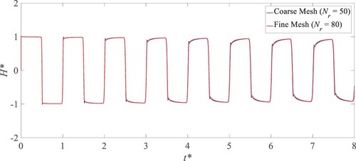
Table 2. System information for Case 1.

Hres (m)	L (m)	R (m)	u0 (m/s)	Re	a (m/s)	Tth (s)	Transient Operation
40	42	0.0362	0.0231	1670	1485	0.1131	sudden close of DV

Table 3. Mesh tests in CFD Fluent for Case 1.

	$\mathrm{\Delta }x$ (m)	Nx	Nr	$\mathrm{\Delta }r$ Growth Rate	$\mathrm{\Delta }t$ (s)
Coarse Mesh	0.1	420	50	1.05	6.73e-5
Fine Mesh	0.1	420	80	1.05	6.73e-5

3.2. Case 2: preliminary numerical verification in the extended blockage case (Zhao et al., 2018)

The second case involves a pipeline system with an antisymmetric extended uniform blockage that only occupies the pipe section’s bottom area. For the blockage section, its centroid $x$, length $l$ and severity/blockage diameter $d$ are listed in Table 4. The mesh scheme listed in Table 5 is the finest one tested in Zhao et al. (2018). In Figure 3, the area-averaged pressure at the pipeline’s outlet agrees well with that shown in Fig. 8 in Zhao et al. (2018). Point C and Point D corresponds to the time that the incident wave propagates upstream, then gets reflected at the extended blockage right and left end, respectively, and finally arrives at the DV.

Figure 3. Area-weighted average pressure trace at the pipe outlet versus time for Case 2

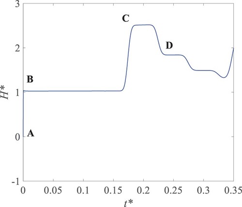
Table 4. System information for Case 2.

							Blockage Parameters
Hres (m)	L (m)	D (m)	u0 (m/s)	Re	a (m/s)	Tth (s)	lb/L	d/D	xb/L	Transient Operation
204	100	0.1	1.0	10^5	1414	0.2829	0.1	0.4	0.6	sudden close of DV

Table 5. Mesh generation scheme in CFD Fluent for Case 2.

$\mathrm{\Delta }x$ (m)	Nx	Nr	$\mathrm{\Delta }r$ Growth Rate	$\mathrm{\Delta }t$ (s)
0.05	2000	50	1.05	3.00e-5

4. Simulation and results

Noticing that radial pressure wave phenomena are not observed in the aforementioned mesh schemes for two preliminary numerical cases in the literature due to the large-scale difference between the axial spatial step $\mathrm{\Delta }x$ and average radial spatial step $\mathrm{\Delta }\overline{r}$. According to (Mitra & Rouleau, 1985), higher and equivalent dimensionless spatial and temporal resolution lead to capture the radial waves, i.e. $\mathrm{\Delta }\xi =\mathrm{\Delta }\eta =\mathrm{\Delta }\tau ,$ where $\mathrm{\Delta }\xi =\mathrm{\Delta }x/R$, $\mathrm{\Delta }\eta =\mathrm{\Delta }\overline{r}/R$ and $\mathrm{\Delta }\tau =a\mathrm{\Delta }t/R$. In this paper, this dimensionless value is set as 0.02 which is small enough to simulate the fluid’s real viscous effect rather than the numerical viscosity in order to observe the radial wave propagation behavior (Che et al., 2018a). Specifically, after careful grid-dependence tests, the corresponding axial mesh number Nx, radial mesh number Nr, and the time step $\mathrm{\Delta }t$. settings are listed in Table 6 and the sketch of the grid scheme is displayed in Figure 4. The convergence presion for the variables in the continuity and momentum equations is set as 10⁻⁶.

Figure 4. Sketch of the selected mesh scheme in CFD model

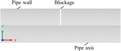
Table 6. Mesh selection in CFD model.

$\mathrm{\Delta }x$ (m)	Nx	Nr	$\mathrm{\Delta }\overline{r}$ (m)	$\mathrm{\Delta }r$ Growth Rate	$\mathrm{\Delta }t$ (s)
4e-4	25000	50	4e-4	1.05	2.69e-7

The steady-state axial velocity profile along the pipe’s axial and radial direction calculated from Ansys Fluent 18.1 is plotted in Figure 5. Axial velocity distribution along the pipe’s axis (see Figure 5(a)) is axisymmetric and fully developed before and after blockage. In Figure 5(b), the computed velocity profile (i.e. numerical result) at the pipe’s outlet satisfies the parabolic distribution (i.e. analytical result) as follows: (6) $u=2\ast u_0\ast (1-(r/R{)}^2)$(6)

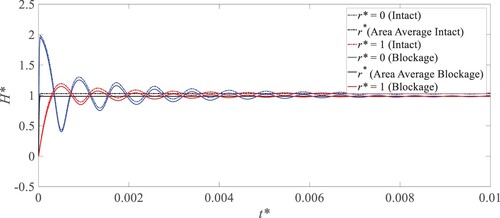
As a comparison, the transient pressure traces during the early stage at different radial locations (r* = 0 corresponds to the axis and r* = 1 is the wall) for the sudden closure of DV in the corresponding intact pipe with L = 10 m and radius R = 0.02 m are plotted in the dashed line in Figure 6 while those for the blockage pipe are plotted in the continuous line. These radial pressure differences (or gradients) observed in these two cases account for the mechanism of the radial pressure waves (Che et al., 2018a). Louati and Ghidaoui (2017) developed the theoretical formula for the propagation angle of these radial waves’ modes, with a zigzag-type path bounded by the pipe wall. Noting that the peak value of the dimensionless pressure at t* = 0 in two cases being up to 2 is due to the axial velocity at the axis being twice the area-averaged velocity (Che et al., 2018a). Besides that, the pressure in the blockage case is slightly lower than that in the intact case, which is due to the steady state pressure drop as a result of the blockage (local energy losses). There is no obvious blockage-induced frequency shift at the pipe axis and wall, though the blockage signature on declining the magnitudes of oscillations is evident. Around t* = 0.01, radial pressure wave vanishes (i.e. no pressure difference between r* = 0 and r* = 1).

Figure 5. Steady-state velocity profile of axial velocity component; (a) along the pipe axis; (b) at the pipe outlet.

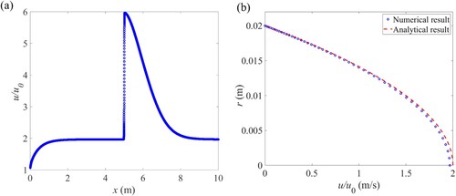
Figure 6. Pressure trace during the early stage of transient process at the pipeline outlet for the sudden DV closure.

4.1. Pressure fields

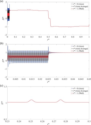
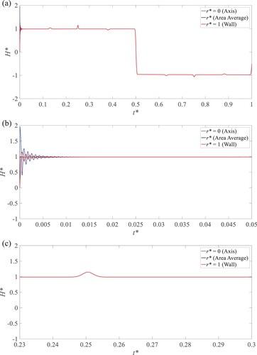
For DV’s HFW oscillation, its oscillation frequency f_in is 1.2 times the radial wave frequency f_r with the oscillation period $t_0^{\ast }$ = 0.025 as shown in Eq. (5). As seen in Figure 7(a), significant pressure differences between the pipe wall and the axis are observed during valve oscillation period. At the beginning of the oscillation, the first maximum peak h* for the axis is up to 2 and the successive peak values quickly decrease to 1.2 during the valve’s oscillation which is different from the result in the intact pipe whose peak values keep nearly 2.0 (Che et al., 2018a). At t*₀, the valve fully closes, and it causes the second maximum peak. Successive pressure wave’s amplitude fast attenuation with the oscillation is due to the fluid’s viscosity and before arriving at the blockage point, the radial waves disappear, acting as plane waves as shown in Figure 7(b). Compared with the corresponding intact case, blockage-induced reflection for these two maximum peaks can be captured by the two minimal peaks that occurred in $t_{C1}^{\ast }$ = 0.25 and $t_{C2}^{\ast }$ = 0.275 (Figure 7(c)). The time $t_{C1}^{\ast }$ indicates the travel time of the plane wavefront between the generation point (valve) and the blockage location, while the time delay between $t_{C1}^{\ast }$ and $t_{C2}^{\ast }$ reflects the DV’s oscillation period.

Figure 7. Pressure trace at the pipe outlet (with blockage) for the HFW oscillation at the DV: (a) in one theoretical period (0 < t* < 1); (b) the enlarged part for 0 < t* < 0.05; (c) the enlarged part for 0.23 < t* < 0.3.

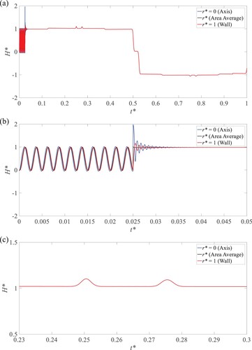
In the low-frequency wave (LFW) oscillation test excited at the DV, except for its oscillation frequency f_in being 0.2 times the radial wave frequency, other parameters keep the same as those of the HFW test. During the valve oscillation period (Figure 8(b)), i.e. 0 < $t_0^{\ast }$ < 0.025, the pressure waves’ oscillation amplitudes are much smaller than those in the HFW test since the radial pressure wave has enough time to influence the cross-sectional pressure profile (Che et al., 2018a). After valve oscillation, similar to the HFW case, two minimum peaks caused by the blockage are observed (Figure 8(c)).

Figure 8. Pressure trace at the pipe outlet (with blockage) for the LFW oscillation at the DV: (a) in one theoretical wave period (0 < t* < 1); (b) the enlarged part for 0 < t* < 0.05; (c) the enlarged part for 0.23 < t* < 0.3.

Noticing the short oscillation of the DV for the HFW and LFW cases and their fast attenuation, that is, after oscillation, no radial waves appear at the blockage. This can be seen from the same pressure traces after $t_0^{\ast }$ > 0.025 in Figures 7 and 8 and the same vorticity behaviors in Figures 13 and 14.

Since the maximum peak generated at the transient initial time for DV’s sudden closure, one minimum peak at $t_0^{\ast }$ = 0.25 (Figure 9(c)) induced by this maximum peak’s reflection at the blockage is observed accordingly.

Figure 9. Pressure trace at the pipe outlet (with blockage) for the sudden DV closure: (a) in one theoretical wave period (0 < t* < 1); (b) the enlarged part for 0 < t* < 0.05; (c) the enlarged part for 0.23 < t* < 0.3.

4.2. Flow fields

The variations of the cross-sectional flow profile during the HFW propagation are studied here. For a pipeline’s intact section (x* = 0.9) which is located at downstream of the blockage section, the axial velocity profiles of the fluid at three time-instants: (i) before (i.e. at t* = 0.0125); (ii) exactly (i.e. at t* = 0.0250); (iii) and after (i.e. at t* = 0.0375) the wavefront arrival are indicated at Figure 10(a). In addition to a reversed flow with an inflection point developing near the wall (Das & Arakeri, 1998), a nearly uniform shift of the axial velocity profile with little change in shape is observed during this deceleration process (Che et al., 2018b; Vardy & Hwang, 1993).

Figure 10. Flow fields at the intact pipe section (x* = 0.9) for three-time sections t* = 0.0125, 0.0250, 0.0375 in red, blue, and pink, respectively; (a) axial velocity field; (b) axial velocity gradient field; (c) radial velocity gradient field; (d) vorticity field.

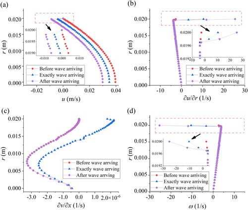
Meanwhile, a significant increase in the axial velocity gradient at the near-wall region is seen from the inset of Figure 10(b) while the axial velocity gradient in the core region keeps nearly zero with time. This time-dependence phenomenon also validates that the near-wall unsteady friction (or unsteady wall shear stress) highly differs from that derived from the quasi-steady flow assumption (Brunone et al., 2000; Vardy & Hwang, 1991). On the other hand, the reversed flow near the wall implies the instantaneous generation of vorticity and its time-dependent diffusion towards the core region (Guerrero et al., 2022). For the radial velocity gradient (in Figure 10(c)), its magnitude of order is small enough compared with that of the axial velocity gradient that can be neglected. As a result, the vorticity field (in Figure 10(d)) at the pipeline’s intact section is dominated by the axial velocity gradient.

Figures 11 and 12 displays the flow fields at the blockage section ($x_b^{\ast }$ = 0.5) during the deceleration and acceleration periods, respectively. For illustration, five characteristic time instants are plotted, in which t* = 0, 0.1250, and 0.2500 represent the initial time, and exact time instants of the positive wavefront’s arrival at the blockage and the upstream reservoir, respectively, and t* = 0.1245, 0.1255 records the time before and after the positive wavefront passing through the blockage. Different from the result shown at the intact section, several key findings are summarized as follows: (i) the nonuniform shift of the axial velocity profile in the boundary layer as shown in Figure 11(a); (ii) the existence of a larger axial velocity gradient and a comparable magnitude of the order of the radial velocity gradient as depicted in Figure 11(b)–(c), which emphasizes the intense of the vorticity diffusion at the blockage. Nevertheless, the vorticity profile (in Figure 11(d)) is still mainly controlled by the axial velocity gradient.

Figure 11. Flow fields at the blocked pipe section during the deceleration period (x* b = 0.5): (a) axial velocity field; (b) axial velocity gradient field; (c) radial velocity gradient field; (d) vorticity field.

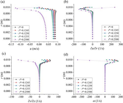
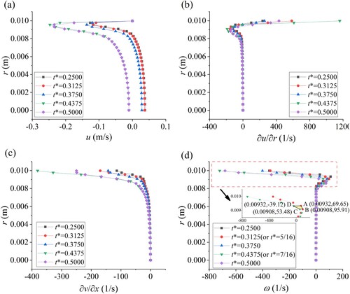
Figure 12. Flow fields at the blocked pipe section during the acceleration period (x* b = 0.5): (a) axial velocity field; (b) axial velocity gradient field; (c) radial velocity gradient field; (d) vorticity field.

4.3. Temporal and spatial evolution of the vorticity field at the blockage

Except for the pressure signal analysis for the user-predefined monitoring points/lines/surfaces, the detailed flow field in the 2D transient simulation can be extracted based on the system-defined physical variables in the Fluent. Here, we focus on the physical quantity, vorticity ω, to which limited attention is paid to transient pipe flows. 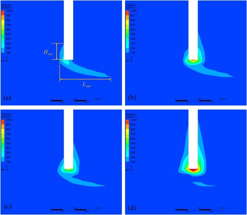It allows for measuring the rotation of a fluid element as it moves in the flow field (Çengel, 2018) (7) $\overrightarrow{\omega }=\mathrm{\nabla }\times \overrightarrow{U}=\text{curl(}\overrightarrow{U}\text{) = }\left(\frac{\mathrm{\partial }v}{\mathrm{\partial }x}-\frac{\mathrm{\partial }u}{\mathrm{\partial }r}\overrightarrow{k}\right)$(7) in which $U=(u,v)$ represents the fluid particle’s velocity vector. Figure 13 visualizes the variation of vorticity magnitude in the vicinity of the blockage during the propagation of the pressure waves. According to the steady-state axial velocity profile results shown in Figure 5(a), the area-averaged Re at the blockage has a value of 2400, which is close to the experimental Re = 2000 in the blocked pipe’s flow conducted by Toophanpour-Rami et al. (2007). The vorticity shape with a long tail demonstrated in this numerical simulation is also observed experimentally with dye visualization by Toophanpour-Rami et al. (2007). Before the arrival of the positive pressure waves coming from downstream, the vorticity distribution already exists and displays the frozen effect as the steady-state (Weinbaum & Parker, 1975). After its passage through the blockage, i.e. from t* = 1/16 to t* = 3/16, the magnitude of vorticity in the region infinitely close to the blockage’s bottom slightly increases and diffuses towards the pipe axis along the radial direction (Ghidaoui & Kolyshkin, 2002), and its height along the blockage’s right side develops twice as seen in Figure 13(b). At t* =  5/16, the negative pressure coming from the reflection of the positive pressure wave at the reservoir doesn’t arrive at the blockage, hence, the vorticity profile remains almost unchanged (Figure 13(c)). After 1/8 t* (i.e. at t^∗ = 7/16 in Figure 13(d)), it gets stronger in the blockage’s local bottom and its effective height H vor approximates to 2/5 of the blockage height.

Figure 13. Vorticity field around the blockage for the HFW oscillation at the DV: (a) t* = 1/16; (b) t* = 3/16; (c) t* = 5/16; (d) t* = 7/16.

In addition, the vortex’s shedding in the axial direction is also observed, evidencing that the vorticity proliferation in DV’s sudden closure in both HFW and LFW cases is the same (the results are not shown to conserve space). This phenomenon could also be explained by the flow fields in the vicinity of the blockage during the wave acceleration stage (i.e. 0.25 < t* < 0.5, see Figure 12). Specifically, the spatial-temporal evolution of the vorticity field for the blockage section $x_b^{\ast }$ = 0.5 with limited radial extent (r_B, r_A) = (r_C, r_D) = (0.00908,0.00932) from t* = 5/16 to t* = 7/16 is marked by a polygon filled with yellow color in Figure 12(d). At t* = 5/16, the vorticity ω varies from 95.91 s⁻¹ to 69.65 s⁻¹, after 1/8T_th, corresponding to the passage of the negative pressure wave, i.e. at t* = 7/16, the vorticity ω at the r_C (or r_B) decreases in magnitude to 53.48 s⁻¹. But for the upper radial location r_D (or r_A), ω not only decreases in magnitude but also has an opposite rotational direction, with a value of – 39.12 s⁻¹, which indicates that a zero vorticity zone must be existent between this radial extent at the specific time.

For better quantification of the spatial variation of vorticity during the first half wave period, three dimensionless parameters that characterize the spatial range of vorticity are defined: (8) $A_{vor}^{\ast }=\frac{A_{vor}}{A_{vor,0}},L_{vor}^{\ast }=\frac{L_{vor}}{R},H_{vor}^{\ast }=\frac{H_{vor}}{R}$(8) where A_vor and $A_{vor,0}^{\ast }$ represent the vorticity area at any time and the initial steady state, respectively; and the axial length L_vor and radial height H_vor (measured from the bottom of the blockage) of vorticity are normalized by the pipe’s radius R. With the aid of the professional java-based image processing program, ImageJ, these quantities (i.e. A_vor, L_vor, and H_vor) could be measured from the picture exported by the CFD-Post. On the whole, as plotted in Figure 16, both $A_{vor}^{\ast }$ shown in Figure 16(a) and $H_{vor}^{\ast }$ shown in the right y-axis of Figure 16(b) exhibit a significant increase after the passage of the positive or negative wave while $L_{vor}^{\ast }$ stays unchanged during the deceleration process until the negative wave disturbing this state.

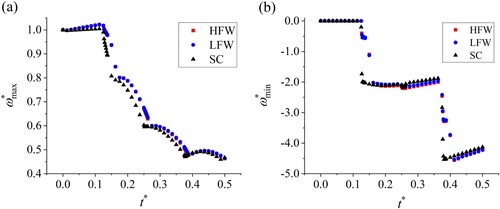
It is worth noting that the vorticity field shown in Figures 13–15 is the Vorticity Magnitude listed in the Quantities table of the Solution Data in CFD-Fluent, according to the definition of vorticity ω in Eq. (7(8) $A_{vor}^{\ast }=\frac{A_{vor}}{A_{vor,0}},L_{vor}^{\ast }=\frac{L_{vor}}{R},H_{vor}^{\ast }=\frac{H_{vor}}{R}$(8) ), its value could be positive or negative, implying anti-clockwise or clockwise rotation of fluid particles in the vicinity of the blockage section. The temporal evolution of the mathematically maximum and minimum vorticity along the blockage section ($x_b^{\ast }$ = 0.5) are plotted in Figure 17, which are normalized by the initial maximum vorticity ωmax,0: (9) ${\omega }_{max}^{\ast }=\frac{{\omega }_{max}}{{{\omega }_{max}}_{,0}},{\omega }_{min}^{\ast }=\frac{{\omega }_{min}}{{\omega }_{max,0}}$(9)

As can be seen from Figure 17, during the first period, ω* max decays continuously after the positive wave passing, which agrees with the left-moving direction of the turning point of the vorticity profile with time proceeding in Figure 11(d). Morton (1984) considers the cross-diffusive annihilation in the fluid as the only mechanism of the vorticity field’s decay. However, for the ${\omega }_{min}^{\ast }$ with the opposite sign, which occurs at the pipe wall (as indicated in Figure 11(d)), a dramatic sudden drop occurs corresponding to the special time instants that the positive or negative wave passing, indicating a sudden increase in the axial velocity gradient in this location. Except for these particular time instants during the investigated period, ω* min may be considered as frozen.

Figure 14. Vorticity field around the blockage for the LFW at the DV: (a) t* = 1/16; (b) t* = 3/16; (c) t* = 5/16; (d) t* = 7/16.

Figure 15. Vorticity field around the blockage for the sudden DV closure: at (a) t* = 1/16; (b) t* = 3/16; (c) t* = 5/16; (d) t* = 7/16.

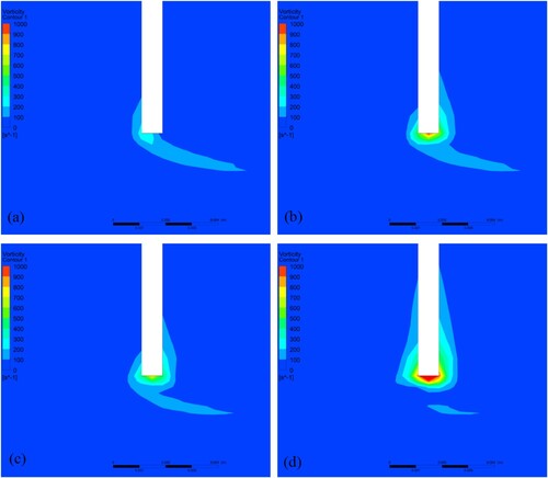
Figure 16. Spatial evolution of the vorticity at the blocked pipe section (x*_b = 0.5): (a) vorticity area; (b) vorticity axial length and radial height.

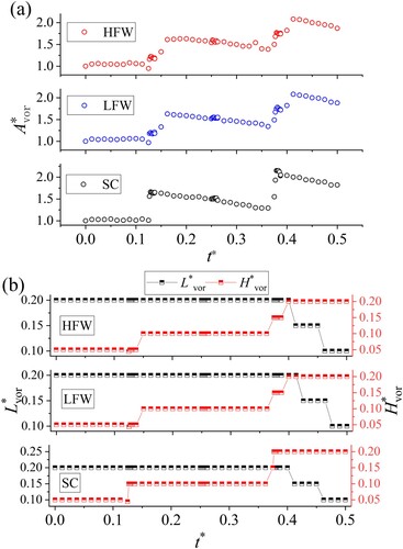
Figure 17. Temporal evolution of the vorticity at the blocked pipe section (x* = 0.5): (a) maximum vorticity; (b) minimum vorticity.

4.4. Wall shear stress

Although wall shear stress can neither generate vorticity nor does it directly influence the variation of vorticity, it relates to vorticity by velocity gradient (Morton, 1984). Besides that, the wall shear stress plays a very important role in transient modeling to predict the pressure trace. Based on these two solid reasons, we quantify the wall shear stress history (τ_w ∼ t*) during the first half wave period at the blockage section ($x_b^{\ast }$ = 0.5) as depicted in Figure 18.

Figure 18. Wall shear stress at the blocked pipe section under different forms of wave oscillation at the DV.

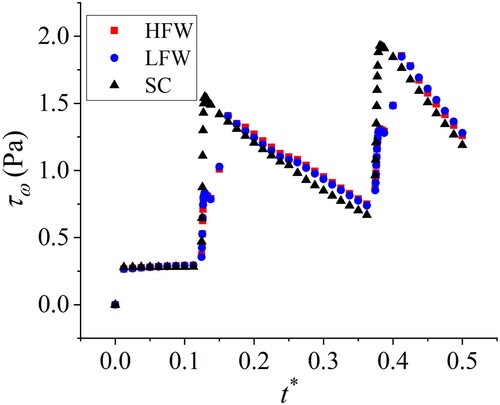
Overall, this figure exhibits a similar trend to that at the pipe’s intact section (Cao et al., 2022; Silva-Araya & Chaudhry, 1997). Similarly, rapid increments in the τ_w are seen just during the arrival of the transient waves. After the wave’s passage, the time-dependent diffusion of the velocity gradient-induced shear stress (viscous forces) towards the core region causes the slow delay of τ_w corresponding to the pre-transition period as explained in the variation of the skin friction coefficient C_f during acceleration of the bulk flow (Guerrero et al., 2021). For demonstration, two sets of peak time instants that relate to the passing of the positive wave from the downstream and the negative wave reflected by the upstream reservoir are extracted (i.e. $t_{P1,SC}^{\ast }$ = 0.1290, $t_{P1,HFW}^{\ast }$ = $t_{P1,LFW}^{\ast }$ = 0.1625, $t_{P2,SC}^{\ast }$ = 0.3830, $t_{P2,HFW}^{\ast }$=$t_{P2,LFW}^{\ast }$ = 0.4125) and comparing these values with the arrival time instants of the positive and negative wavefront (i.e. $t_{P1}^{\ast }$ = 0.1250, $t_{P2}^{\ast }$ = 0.3750) at the blockage section, a local peak time delay is observed (Martins et al., 2018). This time delay provides proof of the inappropriate use of the unsteady friction model in which the unsteady component of τ_w is based on the instantaneous local acceleration.

5. Conclusions

This paper investigates the 2D transient wave behavoirs in a pipeline with discrete (localized) blockage under different wave excitation and flow conditions. The CFD model is established, validated, and applied for this investigation. The results reveal that radial wave behaviors in a transient pipe flow with a discrete blockage (localized) can be observed in this high-resolution mesh scheme and the blockage information can be identified from the wave reflection analysis. Meanwhile, it is also demonstrated that the commonly generated transient wave may develop quickly into a plane wave along the pipeline due to the relatively high frequency and fast attenuation of the induced radial wave. In addition, based on the developed 2D CFD model, the transient wave-blockage interaction has been examined for the local field variables in the vicinity of the blockage for different tested cases. In comparison with intact pipe case, the results of this study on the wave-blockage interaction can be summarized as follows.

• The passage of the pressure wave could induce a nonuniform shift of the axial velocity profile at the blockage section’s near-wall region;

• The magnitude of the radial velocity gradient (∂v/∂x) is nearly ten times larger than that in the intact section, which could approach the order of the axial velocity gradient (∂u/∂r);

• The vorticity fields in the pipe’s intact section and blockage section both highly depend on the fluid’s axial velocity field;

• The extent (area and size) of vorticity, the magnitude of the minimum vorticity, and the wall shear stress at the blockage section present sudden increases after the passage of the positive or negative wave while the magnitude of the maximum vorticity decreases continually with wave time due to its cross-diffusive annihilation.

It is also noted that the results and findings of this study are gained based on the 2D CFD simulation, with an assumption of symmetric blockage configuration and wave generation, as well as rigid pipe wall condition. Further investigations (e.g. 3D model) will be necessary and carried out for more complex situations of blockage configuration and wave generation, such as irregular blockages and multi-path waves in elastic and viscoelastic pipelines.

Notation

Roman letters

a	=	= wave speed (m/s);
A	=	= pipe cross-sectional area (m2);
Avor	=	= area of vorticity (m2);
Cf	=	= skin friction coefficient;
D	=	= pipe diameter (m);
fin	=	= input frequency of the wave (Hz);
fr	=	= a/R radial fundamental wave frequency of a pipeline (Hz);
g	=	= gravitational acceleration (m/s2);
H0	=	= steady-state pressure head (m);
Hjou	=	= Joukovsky head (m);
Hres	=	= pressure head at reservoir (m);
Hvor	=	= radial height of vorticity (m);
H*	=	= dimensionless head perturbation =(H-H0)/Hjou;
lb	=	= uniform blockage length (m);
L	=	= pipe length (m);
Lvor	=	= axial length of vorticity (m);
Q0	=	= initial flow rate from reservoir (m3/s);
Re	=	= Reynolds number;
rb	=	= blockage size (m);
Tth	=	= 4L/a = system theoretical wave period (s);
t*	=	= t/(Tth) = dimensionless time;
u	=	= axial velocity (m/s);
u0	=	= cross-sectional area-averaged axial velocity (m/s);
v	=	= radial velocity (m/s);
x*	=	= x/L = dimensionless location;
xb	=	= blockage location, measured from the reservoir (m);
x*b	=	= xb/L = dimensionless blockage location.

Greek symbols

τw	=	= wall shear stress history (Pa);
ω	=	= vorticity (1/s);

List of abbreviations

DV	=	: downstream valve;
HFW	=	: high-frequency wave;
LFW	=	: low-frequency wave;
Max	=	: maximum;
Min	=	: minimum.
RPV	=	: reservoir-pipeline-valve.
SC	=	: sudden closure;
Vor	=	: vorticity.

Disclosure statement

No potential conflict of interest was reported by the author(s).

Additional information

Funding

This research work was partially supported by the Hong Kong Research Grants Council (RGC project no. 15200719).

References

- Brunone, B., Karney, B., Mecarelli, M., & Ferrante, M. (2000). Velocity profiles and unsteady pipe friction in transient flow. Journal of Water Resources Planning and Management, 126(4), 236–244. https://doi.org/10.1061/(ASCE)0733-9496(2000)126:4(236)
- Cao, Y., Zhou, L., Ou, C., Fang, H., & Liu, D. (2022). 3D CFD simulation and analysis of transient flow in a water pipeline. Journal of Water Supply: Research and Technology-AQUA, 71(6), 751–767. https://doi.org/10.2166/aqua.2022.023
- Çengel, Y. A. (2018). Fluid mechanics: Fundamentals and applications (4th ed.). McGraw-Hill Education.
- Chahardah-Cherik, P., Fathi-Moghadam, M., & Haghighipour, S. (2021). Modeling of transient flows in viscoelastic pipe network with partial blockage. Journal of Water Supply: Research and Technology-AQUA, 70(6). https://doi.org/10.2166/aqua.2021.040
- Chaudhry, M. H. (2014). Applied hydraulic transients, third edition. Springer.
- Che, T. C. (2019). Transient wave behavior in water pipes with non-uniform blockages. Hong Kong Polytechnic University.
- Che, T. C., Duan, H. F., & Lee, P. J. (2021). Transient wave-based methods for anomaly detection in fluid pipes: A review. Mechanical Systems and Signal Processing, 160, 107874. https://doi.org/10.1016/j.ymssp.2021.107874
- Che, T. C., Duan, H. F., Lee, P. J., Meniconi, S., Pan, B., & Brunone, B. (2018a). Radial pressure wave behavior in transient laminar pipe flows under different flow perturbations. Journal of Fluids Engineering, 140(10), 101203. https://doi.org/10.1115/1.4039711
- Che, T. C., Duan, H. F., Lee, P. J., Pan, B., & Ghidaoui, M. S. (2018b). Transient frequency responses for pressurized water pipelines containing blockages with linearly varying diameters. Journal of Hydraulic Engineering, 144(8), 04018054. https://doi.org/10.1061/(ASCE)HY.1943-7900.0001499
- Che, T. C., Duan, H. F., Pan, B., Lee, P. J., & Ghidaoui, M. S. (2019). Energy analysis of the resonant frequency shift pattern induced by nonuniform blockages in pressurized water pipes. Journal of Hydraulic Engineering, 145(7), 04019027. https://doi.org/10.1061/(ASCE)HY.1943-7900.0001607
- Contractor. (1965). The reflection of waterhammer pressure waves from minor losses. Journal of Basic Engineering, 87(2), 445–451. https://doi.org/10.1115/1.3650568
- Das, D., & Arakeri, J. H. (1998). Transition of unsteady velocity profiles with reverse flow. Journal of Fluid Mechanics, 374, 251–283. https://doi.org/10.1017/S0022112098002572
- Duan, H. F. (2016). Sensitivity analysis of a transient-based frequency domain method for extended blockage detection in water pipeline systems. Journal of Water Resources Planning and Management, 142(4), 04015073. https://doi.org/10.1061/(ASCE)WR.1943-5452.0000625
- Duan, H. F., Ghidaoui, M. S., & Tung, Y. K. (2010). Energy analysis of viscoelasticity effect in pipe fluid transients. Journal of Applied Mechanics, 77(4), 044503. https://doi.org/10.1115/1.4000915
- Duan, H. F., Lee, P. J., Ghidaoui, M. S., & Tuck, J. (2014). Transient wave-blockage interaction and extended blockage detection in elastic water pipelines. Journal of Fluids and Structures, 46, 2–16. https://doi.org/10.1016/j.jfluidstructs.2013.12.002
- Duan, H. F., Lee, P. J., Ghidaoui, M. S., & Tung, Y. K. (2012). Extended blockage detection in pipelines by using the system frequency response analysis. Journal of Water Resources Planning and Management, 138(1), 55–62. https://doi.org/10.1061/(ASCE)WR.1943-5452.0000145
- Duan, H. F., Pan, B., Wang, M. L., Chen, L., Zheng, F. F., & Zhang, Y. (2020). State-of-the-art review on the transient flow modeling and utilization for urban water supply system (UWSS) management. Journal of Water Supply: Research and Technology-AQUA, 69(8), 858–893. https://doi.org/10.2166/aqua.2020.048
- Ferreira, J. P. B., Martins, N. M., & Covas, D. I. (2018). Ball valve behavior under steady and unsteady conditions. Journal of Hydraulic Engineering, 144(4), 04018005. https://doi.org/10.1061/(ASCE)HY.1943-7900.0001434
- Ghidaoui, M. S., & Kolyshkin, A. A. (2002). A quasi-steady approach to the instability of time-dependent flows in pipes. Journal of Fluid Mechanics, 465, 301–330. https://doi.org/10.1017/S0022112002001076
- Guerrero, B., Lambert, M. F., & Chin, R. C. (2021). Transient dynamics of accelerating turbulent pipe flow. Journal of Fluid Mechanics, 917, A43. https://doi.org/10.1017/jfm.2021.303
- Guerrero, B., Lambert, M. F., & Chin, R. C. (2022). Extension of the 1D unsteady friction model for rapidly accelerating and decelerating turbulent pipe flows. Journal of Hydraulic Engineering, 148(9), 04022014. https://doi.org/10.1061/(ASCE)HY.1943-7900.0001998
- Jewell, N., & Denier, J. P. (2013). The decay of the flow in the end region of a suddenly blocked pipe. Journal of Fluid Mechanics, 730, 533–558. https://doi.org/10.1017/jfm.2013.360
- Keramat, A., & Zanganeh, R. (2019). Statistical performance analysis of transient-based extended blockage detection in a water supply pipeline. Journal of Water Supply: Research and Technology-AQUA, 68(5), 346–357. https://doi.org/10.2166/aqua.2019.014
- Kim, S. H. (2018). Multiple discrete blockage detection function for single pipelines. 3rd EWaS international conference, Lefkada Island, Greece.
- Kim, S. H. (2022). Dimensionless impedance method for the transient response of pressurized pipeline system. Engineering Applications of Computational Fluid Mechanics, 16(1), 1641-1654. https://doi.org/10.1080/19942060.2022.2108500
- Lai, Z., Louati, M., Nasraoui, S., & Ghidaoui, M. (2021). Numerical investigation of high frequency wave-leak interaction in water-filled pipes. Journal of Hydraulic Engineering, 147(1), 04020091. https://doi.org/10.1061/(ASCE)HY.1943-7900.0001835
- Lee, P. J., Vítkovský, J. P., Lambert, M. F., Simpson, A. R., & Liggett, J. A. (2008). Discrete blockage detection in pipelines using the frequency response diagram: Numerical study. Journal of Hydraulic Engineering, 134(5), 658–663. https://doi.org/10.1061/(ASCE)0733-9429(2008)134:5(658)
- Liu, G., Zhang, Y., Knibbe, W. J., Feng, C., Liu, W., Medema, G., & Van Der Meer, W. (2017). Metabolic responses of the growing daphnia similis to chronic AgNPs exposure as revealed by GC-Q-TOF/MS and LC-Q-TOF/MS. Water Research, 114(116), 135–143. https://doi.org/10.1016/j.watres.2017.02.046
- Liu, X. F., Gong, C. C., Zhang, L. T., Jin, H. Z., & Wang, C. (2020). Numerical study of the hydrodynamic parameters influencing internal corrosion in pipelines for different elbow flow configurations. Engineering Applications of Computational Fluid Mechanics, 14(1), 122–135. https://doi.org/10.1080/19942060.2019.1678524
- Louati, M., & Ghidaoui, M. S. (2017). High-frequency acoustic wave properties in a water-filled pipe. Part 1: Dispersion and multi-path behaviour. Journal of Hydraulic Research, 55(5), 613–631. https://doi.org/10.1080/00221686.2017.1354931
- Louati, M., Meniconi, S., Ghidaoui, M. S., & Brunone, B. (2017). Experimental study of the eigenfrequency shift mechanism in a blocked pipe system. Journal of Hydraulic Engineering, 143(10), 04017044. https://doi.org/10.1061/(ASCE)HY.1943-7900.0001347
- Martins, N. M. C., Brunone, B., Meniconi, S., Ramos, H. M., & Covas, D. I. C. (2018). Efficient computational fluid dynamics model for transient laminar flow modeling: Pressure wave propagation and velocity profile changes. Journal of Fluids Engineering, 140(1), 011102. https://doi.org/10.1115/1.4037504
- Martins, N. M. C., Carrico, N. J. G., Ramos, H. M., & Covas, D. I. C. (2014). Velocity-distribution in pressurized pipe flow using CFD: Accuracy and mesh analysis. Computers & Fluids, 105, 218–230. https://doi.org/10.1016/j.compfluid.2014.09.031
- Martins, N. M. C., Soares, A. K., Ramos, H. M., & Covas, D. I. C. (2016). CFD modeling of transient flow in pressurized pipes. Computers & Fluids, 126, 129–140. https://doi.org/10.1016/j.compfluid.2015.12.002
- Meniconi, S., Brunone, B., Ferrante, M., & Massari, C. (2012). Transient hydrodynamics of in-line valves in viscoelastic pressurized pipes: Long-period analysis. Experiments in Fluids, 53(1), 265–275. https://doi.org/10.1007/s00348-012-1287-3
- Meniconi, S., Brunone, B., Ferrante, M., & Massari, C. (2014). Energy dissipation and pressure decay during transients in viscoelastic pipes with an in-line valve. Journal of Fluids and Structures, 45, 235–249. https://doi.org/10.1016/j.jfluid-structs.2013.12.013
- Mitra, A., & Rouleau, W. (1985). Radial and axial variations in transient pressure waves transmitted through liquid transmission lines. Journal of Fluids Engineering, 107(1), 105–111. https://doi.org/10.1115/1.3242423
- Morton, B. R. (1984). The generation and decay of vorticity. Geophysical & Astrophysical Fluid Dynamics, 28(3–4), 277–308. https://doi.org/10.1080/03091928408230368
- Pan, B., Duan, H. F., Meniconi, S., & Brunone, B. (2021). FRF-based transient wave analysis for the viscoelastic parameters identification and leak detection in water-filled plastic pipes. Mechanical Systems and Signal Processing, 146, 107056. https://doi.org/10.1016/j.ymssp.2020.107056
- Pan, B., Duan, H. F., Meniconi, S., Urbanowicz, K., Che, T. C., & Brunone, B. (2020). Multistage frequency-domain transient-based method for the analysis of viscoelastic parameters of plastic pipes. Journal of Hydraulic Engineering, 146(3), 04019068. https://doi.org/10.1061/(ASCE)HY.1943-7900.0001700
- Shao, Z. S., & Yost, S. A. (2018). Numerical investigation of driving forces in a geyser event using a dynamic multi-phase navier–stokes model. Engineering Applications of Computational Fluid Mechanics, 12(1), 493–505. https://doi.org/10.1080/19942060.2018.1459322
- Silva-Araya, W. F., & Chaudhry, M. H. (1997). Computation of energy dissipation in transient flow. Journal of Hydraulic Engineering, 123(2), 108–115. https://doi.org/10.1061/(ASCE)0733-9429(1997)123:2(108)
- Stephens, M. L., Simpson, A. R., & Lambert, M. F. (2007). Hydraulic transient analysis and discrete blockage detection on distribution pipelines: Field tests, model calibration, and inverse modeling. World environmental and water resources congress 2007, Tampa, Florida.
- Toophanpour-Rami, M., Hassan, E., Kelso, R., & Denier, J. (2007). Preliminary investigation of impulsively blocked pipe flow. 16th australasian fluid mechanics conference, Crowne Plaza, Gold Coast, Australia.
- Vardy, A. E., & Hwang, K. L. (1991). A characteristics model of transient friction in pipes. Journal of Hydraulic Research, 29(5), 669–684. https://doi.org/10.1080/00221689109498983
- Vardy, A. E., & Hwang, K. L. (1993). A weighting function model of transient turbulent pipe friction. Journal of Hydraulic Engineering, 31(4), 533–548.
- Wang, C., Nilsson, H., Yang, J., & Petit, O. (2017). 1D–3D coupling for hydraulic system transient simulations. Computer Physics Communications, 210, 1–9. https://doi.org/10.1016/j.cpc.2016.09.007
- Weinbaum, S., & Parker, K. H. (1975). The laminar decay of suddenly blocked channel and pipe flows. Journal of Fluid Mechanics, 69(4), 729–752. https://doi.org/10.1017/S0022112075001668
- Xu, H. L., Chen, W., & Hu, W. G. (2020). Hydraulic transport flow law of natural gas hydrate pipeline under marine dynamic environment. Engineering Applications of Computational Fluid Mechanics, 14(1), 507–521. https://doi.org/10.1080/19942060.2020.1727774
- Yan, X. F., Duan, H. F., Wang, X. K., Wang, M. L., & Lee, P. J. (2021). Investigation of transient wave behavior in water pipelines with blockages. Journal of Hydraulic Engineering, 147(2), 04020095. https://doi.org/10.1061/(ASCE)HY.1943-7900.0001841
- Yu, M. H., Wang, R., Liu, K., & Yao, J. F. (2019). Numerical simulation of three-dimensional transient flow characteristics for a dual-fluid atomizer. Engineering Applications of Computational Fluid Mechanics, 13(1), 1144–1152. https://doi.org/10.1080/19942060.2019.1666302
- Zhao, M., Ghidaoui, M. S., Louati, M., & Duan, H. F. (2018). Numerical study of the blockage length effect on the transient wave in pipe flows. Journal of Hydraulic Research, 56(2), 245–255. https://doi.org/10.1080/00221686.2017.1394374
- Zhou, L., Liu, D. Y., & Ou, C. Q. (2011). Simulation of flow transients in a water filling pipe containing entrapped air pocket with VOF model. Engineering Applications of Computational Fluid Mechanics, 5(1), 127–140. https://doi.org/10.1080/19942060.2011.11015357
- Zouari, F., Blåsten, E., Louati, M., & Ghidaoui, M. S. (2019). Internal pipe area reconstruction as a tool for blockage detection. Journal of Hydraulic Engineering, 145(6), 04019019. https://doi.org/10.1061/(ASCE)HY.1943-7900.0001602