Experimental and numerical investigation of flow distribution pattern at a T-shape roadway crossing under extreme storms

ABSTRACT

A major drainage systemwhich uses urban roadways as flood passages during extreme storm events has been proven to be effective and low-cost. However, to date, the amount of flow diverted at a bifurcating road crossing still could not be accurately assessed. Previous studies mainly focused on diversion flat bottom channels with no turning radius. Results from these studies are not applicable to the road crossing due to the significant discrepancies between the two flow fields. In this study, the flow distribution pattern at a roadway crossing with a T-shape was studied experimentally and numerically. The three-dimensional computational fluid dynamics (CFD) model was constructed using FLUENT. The numerical model was validated using the experimental results and showed satisfying agreements. Results of the 2^k factorial design experiments show that the flow distribution ratio is sensitive to turning radius,  longitude slope,  flowrate and downstream boundary conditions. Detailed numerical studies were conducted to reveal the relationship between the flow distribution ratio and the individual impacting factor. Findings from this research could provide more accurate flowrate predictions  to  guide the design of the road crossings to improve the performance of the major drainage system during extreme storms.

Keywords:

• CFD
• urban flooding
• major drainage system
• road crossing
• extreme storms

1. Introduction

Urban flooding, caused by urbanization process and global climate change, poses high risks to facilities and public safety throughout the world more frequently than ever (Chen et al., 2015; Li et al., 2021; Tellman et al., 2021). According to researches on global climate changes (Kourtis & Tsihrintzis, 2021), urban flood risk is expected to be more devastating in the future as a result of increasing extreme storms. Traditional flooding mitigation practices include upgrading the storm water drainage network and constructing detention basins. These practices are effective yet expensive to implement in an urban setting, especially in the well-developed regions due to very limited land available for additional infrastructures.

These limitations could be overcome by constructing a major drainage network in the urban areas (Schmitt, et al., 2004; Mignot et al., 2019; Tahvildari et al., 2022). A major drainage network uses urban roadways as surface passages to effectively transport high volume of floods during extreme storms. The major drainage system works together with the traditional drainage network and forms a dual drainage system. In another word, if the storm is an ordinary rainfall event, stormwater will be drained through the traditional drainage network while in extreme storms, the portion of stormwater that exceeds the capacity of the drainage network will be drained through roadways. Due to the large flow cross section area a roadway provides, the roadway major drainage system is a cost-effective way to mitigate flooding (Chang et al., 2018; Li et al., 2021). However, using a roadway as a stormwater passage creates risks as well. As the excess runoff flows along the roadways, it creates safety hazards to pedestrians and vehicles because of potential slipping and flipping risks because of hydroplaning phenomenon. Hence, the flowrate carried by roadways needs to be precisely predicted and limited below an allowable level for safety purpose (Shams et al., 2020).

However, flowrate on some urban roadways could not be accurately assessed due to knowledge gaps. These roadways are the downstream roadways of a road crossing with two outlets, for example, a T-shape road crossing with one road flowing in and two roadways flowing out. To date, the amount of flow diverted by the branch road is still unknown to engineers and scientists. This seems odd because quite a few researches have been carried out in the flow filed of a diversion channel. A diversion channel is very similar to a T-shape road crossing. In both configurations, flow is re-distributed at the crossing. Studies on flow diversion channel has been used to guide engineering practices on irrigation and drainage network system, water supplying plants etc. (Neary & Odgaard, 1993). Studies on diversion channels include theoretical study by Hsu et al. (2002), experimental studies by Ramamurthy and Satish (1988), Neary and Odgaard (1993), Nania et al. (2004) and Rivière et al. (2006), two-dimensional numerical studies by Shettar and Murthy (1996) and Momplot et al. (2017), and three-dimensional studies by Ramamurthy et al. (2007), Sharifipour et al. (2015) and Li and Zeng (2009).

However, the results on diversion channels are not completely applicable to road crossings. This is due to the noticeable discrepancies in the channel geometries. First, in the diversion channel system, the two channels intersect without a turning radius while two roads always cross each other with a turning radius for traffic safety purpose. Second, the channel in the existing studies has a flat bottom while the roadway always has a side slope that promotes drainage in the lateral direction to minimize water ponding on the paved surface (Shams et al., 2020). The combination of turning radius and side slope results in a much more complicated flow field in the roadway crossing configurations. On one hand, the existence of the turning radius smoothens streamlines that enter the branch channel, which could reduce or the size of the separation zone on the branch channel or even eliminate it. As shown by Neary and Odgaard (1993), in cases of the straight cut diversion channels, separation zones appear in both main channel and branch channel, which greatly reduce the effective flow area. In a study on flow separation zone at the branch channel, Shettar and Murthy (1996) tentatively compared the streamlines in a straight-cut diversion channel and in a channel intersection with a turning radius. Their study revealed that in cases the turning radius present, the recirculation zone on the branch almost disappeared, which promoted more flow into the branch channel. However, their study did not focus on the flowrate distribution side nor include the roadway side slope. On the other hand, the cross slope of the roadway creates a lateral velocity vector that leads to a secondary flow in the vertical direction according to White and Island (2011). The cross slope also creates a triangle flow area cross-section wise near the curb sides, which causes water depth along the transverse direction distribute unevenly. This would affect the flow field at the crossing as well. To date, how the turning radius and the cross slope influence the flowrate distribution ratio is still unknown. This poses a big challenge when it comes to design a roadway crossing for safely transporting excess flood purpose, especially during extreme storm events.

Besides turning radius and side slope, other roadway design parameters, such as the upstream and downstream roadway longitude slope, as well as operational conditions including inflow flowrate and boundary conditions also contribute to the flow distribution ratio at road crossings. Previous studies on the flat bottom diversion channel system could help to understand the potential impacting factors. Ramamurthy et al. (1990) found out that the portion of flow diverted to the branch channel is related to Froude number in both upstream and downstream channels when the inflow Froude number is low. Mizumura et al. (2003) further found that the flow diversion ratio is only affected by Froude number of the upstream channel if the flow is supercritical along the whole channel. Later, Abderrezzak et al. (2011) and Rivière et al. (2014) revealed experimentally that if the flow translates from a supercritical state to a subcritical state, the flow diversion ratio is a function of both upstream and downstream Froude number.

Based on the literature review, it could be guessed that potential factors contributing to the flow distribution ratio at a T-shape road crossing include roadway geometry parameters (turning radius, side slope, longitude slope) and operational conditions (inflow flowrate, downstream boundary conditions). This means the flow distribution is a function of five impacting factors, as shown in Eq (1). (1) $R_q=f(\text{R},S_x{S}_y,Q_u,B{C}_{down})$(1) Where $R_q$ is flow distribution ratio, R is turning radius, S_x is roadway side slope, S_y is roadway longitude slope, $B{C}_{down}$ is downstream boundary condition.

It could be seen from Eq. (1) that to understand the relationship between $R_q$ and all the impacting factors requires a large number of experiments to be conducted. It is not cost effective to set up physical models for all the experiments. Numerical simulation is the ideal alternative for the physical experiments in this study. Previous studies showed that two-dimensional numerical models that solve the Shallow Water Equations are less capable of capturing the complex flow conditions such as the secondary flow and separation in this study. As confirmed experimentally by Neary and Odgaard (1993) and Ramamurthy et al. (2007), diversion flow has a distinct three-dimensional structure. In addition, in the three-dimensional numerical study of a 90° confluence channel junction solving the RANS equations and k-ω turbulence closures by Huang et al. (2002), shows that although two-dimensional method is appropriate for low flowrate cases, a full three-dimensional model is needed to capture the flow physics in higher flowrate cases. Kesserwani et al. (2010) simulated the flow field at a four-branch crossroad using a Runge–Kutta discontinuous Galerkin (RKDG) finite element method to solve RANS equations and found the numerical simulation results match the experimental results well. Sharifipour et al. (2015) investigated velocity and flowmeter measurement accuracy at open-channel junctions that is impacted by the channel width and discharge ratio based on a three-dimensional Ansys-CFX model. Hence, the three-dimensional CFD simulation is necessary to investigate deeply into the flow field.

In this study, the flow distribution pattern at a roadway crossing with a T-shape was studied experimentally and numerically. The goal of this study is to reveal the influence of key roadway design parameters including turning radius, cross slope, and longitudinal slopes under different flowrate scenarios and boundary conditions. A physical model of a T-shape road crossing was established. The corresponding CFD model was constructed using FLUENT. Results from the physical experiments were used to validate the numerical CFD model. Conclusions from this study could be used to assist civil engineers in future planning and designing urban roadway crossings to construct a more efficient and effective flood conveyance system to alleviate urban inner flooding. This work is important because the implement of a roadway major drainage system significantly promotes the capacity of existing drainage system so that the city is more resilient in handling extreme storms.

2. Methodologies

2.1. Experimental setup

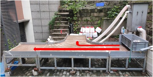
To investigate the influence of roadway design parameters, a physical model of a T-shape road crossing has been set up in this study. The goal of the physical experiments is to validate the numerical model as well as sheds lights on the understanding of the complex flow field. The experimental setup is demonstrated in Figure 1. A site photo of the system is shown in Figure 2. The system consists of a main road and a branch road. The two roads intersect at a right angle and form a T-shape road crossing. The upstream of the main road is the inflow side while the downstream main road and the branch are the outflow sides. Each roadway has a same width (B) of 0.9 m. The turning radius R is 0.6 m. The lengths of the roads L₁ upstream and downstream the crossing is 1.0 m, respectively. Elevation at the inflow side and the two outflow sides of the system could be adjusted separately to vary the longitude slopes. In all experiments, a longitudinal slope S_y1 = S_y2 = 1% was used inside of the crossing area, as depicted in Figure1. A side slope (S_x) of 1.5% is used for all roadways.

Figure 1. Schematic of the experimental system.

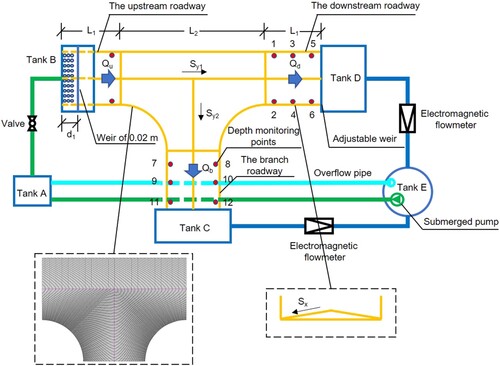
Figure 2. Site photo of the experimental setups.

The experimental apparatus includes a submersible pump with a rated flow of 50 m/h and a lift of 10 m, two DN65 electromagnetic flowmeters with a measuring range from 0 to 50 m³/h and an error level of ±0.5%. As demonstrated in Figure 1, the inflow was pumped from tank E to tank A. The inflow Q_u was divided into Q_d and Q_b by downstream road and branch road respectively and returned to tank E. Measurements were conducted after the system reaches a steady flow state. Flowrate in the downstream channels (Q_b and Q_d) was measured using electromagnetic flowmeters set. Twelve water depth monitors are established, as shown as red dots in Figure 1, to obtain the water depth data to calibrate the numerical models. The depth was measured using a steel ruler with an accuracy of 0.5 mm. The whole system was constructed of PVC material. The bed of the roadway was finished with cement mortar smoothly so that it has the corresponding roughness.

2.2. Numerical model

In this study, a numerical model was constructed to extensively investigate the influence of the design parameters and the working conditions.

2.2.1. Governing equations

The numerical model was constructed using Ansys Fluent 19.0 (Fluent, 2018), which solves the unsteady three-dimensional Reynolds-averaged Navier–Stokes (RANS) equations using the finite volume method. The governing equations are shown as below: (2) $\begin{array}{rl}\frac{\mathrm{\partial }{u}_i}{\mathrm{\partial }{x}_i}& =0\end{array}$(2) (3) $\begin{array}{rl}\frac{\mathrm{\partial }{u}_i}{\mathrm{\partial }t}+u_j\frac{\mathrm{\partial }{u}_i}{\mathrm{\partial }{x}_j}& =-\frac{1}{\rho }\frac{\mathrm{\partial }p}{\mathrm{\partial }{x}_i}+\frac{\mathrm{\partial }}{\mathrm{\partial }{x}_j}\left[v\left(\frac{\mathrm{\partial }{u}_i}{\mathrm{\partial }{x}_j}+\frac{\mathrm{\partial }{u}_j}{\mathrm{\partial }{x}_i}\right)\right]\\ & -\frac{\mathrm{\partial }}{\mathrm{\partial }{x}_j}(\overline{{u^{\mathrm{\prime }}}_i{u^{\mathrm{\prime }}}_j})\end{array}$(3) where p = pressure; u_i= mean velocity in the x_i direction (i =  1,2,3) and $u_i^{\mathrm{\prime }}$ is the corresponding fluctuating components, $\overline{u{}_i^{\mathrm{\prime }}u{}_j^{\mathrm{\prime }}}$ is the Reynolds stresses in turbulence simulation.

2.2.2. Turbulent model

In this study, the Boussinesq hypothesis was used to relate Reynolds stresses to the mean velocity gradients to close the RANS equations. (4) $\begin{array}{r}-\rho \overline{{u^{\mathrm{\prime }}}_i{u^{\mathrm{\prime }}}_j}={\mu }_t\left(\frac{\mathrm{\partial }{u}_i}{\mathrm{\partial }{x}_j}+\frac{\mathrm{\partial }{u}_j}{\mathrm{\partial }{x}_i}\right)-\frac{2}{3}\left(\rho k+{\mu }_t\frac{\mathrm{\partial }{u}_i}{\mathrm{\partial }{x}_i}\right){\delta }_{ij}\end{array}$(4)

In the research work of Younus and Hanif Chaudhry (1994) and Azimi and Shabanlou (2015), k-ε model was recommended for the simulation of flow turbulence in open channel flow due to its high accuracy in the simulation of flow with high stress. In later simulations, Sharifipour et al. (2015) compared the performance of standard k-ε, RNG k-ε, and k-ω and found the RNG k-ε model worked better than the standard k-ε model. In the trial tests prior to the numerical experiments in this study, the RNG k-ϵ model was found to have the best convergence performance. Hence, RNG k-ϵ model was used in all simulations. In a k-ϵ model, μ_t is computed as a function of the turbulence kinetic energy k and the turbulence dissipation flowrate ε: (5) $\begin{array}{r}{\mu }_t=\rho C_{\mu }\frac{k^2}{\epsilon }\end{array}$(5)

2.2.3. Boundary conditions

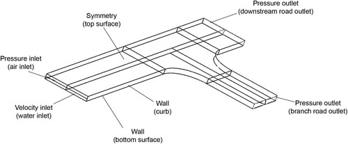
The boundary conditions in all simulations are shown in Figure 3. To reduce the influence from the inlet boundary, the upstream roadway was extended by extra 3.0 m in the numerical model. The inflow boundary at the upstream was set for both water and air phases. For the water phase, a uniform velocity profile with a value of the mean-velocity was used. For the air phase, a pressure inlet with a zero Pascal gauge pressure was prescribed. For the outlet boundary, the pressure outlet was specified downstream of the channel. A non-slip boundary condition was used for all the walls (channel bottom, sidewalls, and weir). A symmetric boundary was applied at the top of the computational domain.

Figure 3. Boundary conditions of CFD model.

2.2.4. Computational mesh

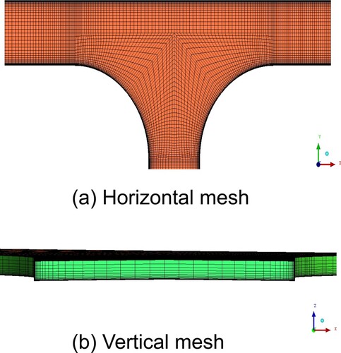
Structural hexahedral meshes were used in this study. The computational mesh was generated in such a way so that the size of the mesh along the length, width and height direction is approximately 5.0, 5.0 and 1.0 cm, respectively. A finer mesh was used in regions close to the junction and the walls, where significant velocity gradients are expected. The final number of grids is around 200,000, fluctuating as the design parameters change. A typical computational mesh in this study is shown in Figure 4.

Figure 4. Computational mesh in the horizontal and vertical directions.

2.2.5. Solution procedure

An implicit finite volume method was used to solve the governing equations in FLUENT while A PISO algorithm was used to decouple velocity and pressure field. The convection terms in the momentum equations were discretized using a second order upwind scheme while a first-order upwind scheme was used in the k-ϵ transport equations. A PRESTO pressure discretization was used to solve the decoupled pressure equation because of the best convergence shown in the trial tests. The volume of fluid (VOF) model was adopted to track the moving free surface. Time step size was specified to be 0.01 s based on the Courant number restriction (CFL). The simulation continued until a steady-state was achieved.

2.3. Impacting factor sensitivity analysis

Because multiple impacting factors are involved in the flow distribution process as described above, a 2^k factorial design test (Montgomery, 2005) was carried out first to screen the key factors (or more sensitive factors) that need to have a detailed study. Results from the 2^k factorial design experiments could be used to reduce the total amount of simulation runs by filtering the less sensitive factors.

Based on the 2^k factorial design theory, two levels were selected for each factor, as shown in Table 1. Because boundary condition is only a sensitive factor in subcritical flow, it is not included in the factorial design but included in later simulations. This results to a total of 2⁴ which is 16 combinations. Numerical simulations were first carried out based these 16 combinations. Setup of the 2k factorial design experiments is shown in Table 2. The low and high levels of the road design parameters were determined based on the national design standard of urban roadways in China (Mohurd, 2011). For example, a low S_y represents a flat region while a high S_y represents a mountainous region with steep slopes. The lower and higher limits of the flowrate were selected so that both subcritical and supercritical flow regimes are covered. 

Table 1. Factors and levels selected for the 2^k factorial design experiments.

Factors	Low level (−1)	High level (+1)
Qu(m^3/h)	10	40
Sy(%)	0.3	5
Sx(%)	1	2
R(m)	1.3	3.2

Table 2. Setups of the 2^k factorial design experiments.

ID	Qu(m^3/h)	Sy(%)	Sx(%)	R(m)
1	10	0.3	1	1.3
2	10	0.3	1	3.2
3	10	0.3	2	1.3
4	10	0.3	2	3.2
5	10	5	1	1.3
6	10	5	1	3.2
7	10	5	2	1.3
8	10	5	2	3.2
9	40	0.3	1	1.3
10	40	0.3	1	3.2
11	40	0.3	2	1.3
12	40	0.3	2	3.2
13	40	5	1	1.3
14	40	5	1	3.2
15	40	5	2	1.3
16	40	5	2	3.2

3 Validation of numerical models

Performance of the developed CFD model was validated using experimental results under three slope settings. A total of nine cases were used to compare the simulated results and the measured experimental results. Parameter combinations used in the CFD model validation tests are shown in Table 3.

Table 3. Parameter combinations used in the CFD model validation tests.

Longitude Slopes (Sy)	Upstream inflow flowrate Qu (m^3/h)
1%	24.85	46.55	4.99
3%	24.22	16.47	4.81
5%	24.30	14.88	4.48

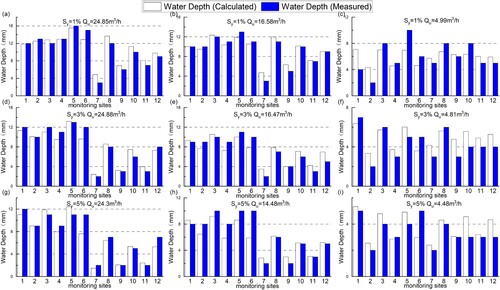
Figure 5 compared the flow distribution ratio from the experimental measurements and numerical predictions. As indicated by Figure 4, the computed results by the numerical model are quite close to the experimental measurements. The numerical error is within 10% of the measurements. Water depths measured in experiments at the 12 monitoring sites were plotted against the numerically simulation results in Figure 6. It could be seen from this figure that the developed numerical model accurately predicted the water depth variation along the channel under various slopes and inflow flowrate combinations. The numerical results match the experimental measurements very well.

Figure 5. Comparison of experimental results and numerical predictions: (a) flow distribution ratio; (b) water depth, where A1 is 1% longitude slope, A2 is3% longitude slope, and A3 is 5% longitude slope for all roadways.

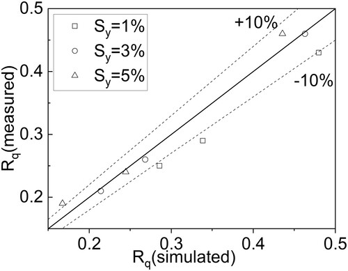
Figure 6. Comparison of water depth measured experimentally and predicted numerically along the channel.

Performance of the CFD model was also assessed quantitatively by calculating the Nash-Sutcliffe Efficiency Coefficient (NSE) and Root Mean Square Error (RSME) using the following formula: (6) $\begin{array}{rl}NSE& =1-\frac{\sum {(Y_{simulated}-Y_{measured})}^2}{\sum {(Y_{measured}-\overline{Y_{measured}})}^2}\end{array}$(6) (7) $\begin{array}{rl}RSME& =\sqrt{\frac{1}{N}\sum {(Y_{simulated}-Y_{measured})}^2}\end{array}$(7)

Where $Y_{simulated}$ is the value predicted by the CFD model, $Y_{measured}$ is the value measured in the physical experiment, and the $\overline{Y_{measured}}$ is the mean value of the measured value.

A value of 0.93 and 0.92 of NSE were obtained for flow distribution ratio and water depth. The values are close to 1.0 which means the model predictions are close to measured data. The RSME of flow distribution is 0.028, about 5-10% of the flow distribution ratio, which ranges between 0.2 and 0.5 in all experiments. The RSME of water depth is 1.6 mm, about 15% of the water depth. In conclusion, the developed CFD model could accurately simulate the flow field at a T-shape road crossing.

4. Results and discussions

4.1. Results of impacting factor sensitivity test

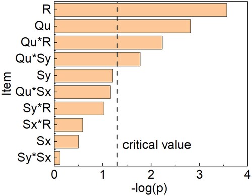
Results of the 2^k factorial design experiments were analyzed using the statistical software SPSS. The sensitivity of each factor and the factor combinations in the determination of the flowrate distribution ratio were shown in Figure 8 in the form of a Pareto chart. The x-axis -log(p) represents the significance of each variable in the flowrate distribution process. The dash line with a -log(p) value of 1.25 represents the threshold that a variable is important to the flowrate distribution ratio. Figure 7 shows that the significance of variables ranges from high to low are turning radius R, upstream flowrate Q_u, combination Q_u* S_y, and combination Q_u* R respectively. It is a surprise that the side slope of S_x does not show strong influences as expected when it comes to flowrate distribution ratio. Also, the longitude slope (S_y) has a value less than 1.25 which means it does not impact the flowrate distribution that much. However, it shows strong interactions with the flowrate. Hence the longitude slope (S_y) is analyzed in later simulations.

Figure 7. Pareto chart results of 2^k factorial design experiments, where the dash line represents the threshold that a variable is considered to be important to the flowrate distribution ratio.

Hence, in the following full sequence test, these three factors were studied. Four level were selected for each of the three factors. This results a total numerical simulation runs of 4³ = 64. The simulated factors and level values are shown in Table 4. After excluding the insignificant influencing factors, a multi-level full sequence test was established to explore the influence of each key factors.

Table 4. Factors and levels used in the multi-level full sequence simulations.

Factors	Three levels of factor values	Description
R(m)	1.3, 2, 2.6, 3.2	Roadway turning radius
Sy(%)	0.3, 1, 3, 5	Roadway longitude slope
Qu(m^3/h)	10, 20, 30, 40	Upstream inflow flowrate

4.2. Influence of roadway turning radius

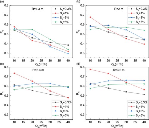
Figure 8 shows how distribution ratio (R_q) varies with the upstream inflow flowrate Q_u at different turning radius R where the longitude slope S_y is fixed. The computed stream patterns at the crossing under different combinations of turning radius R and longitude slope S_y were plotted in Figure 9.

Figure 8. Relationship of distribution ratio R_q versus inflow flowrate Q_u at different turning radius R when longitude slope S_y is fixed.

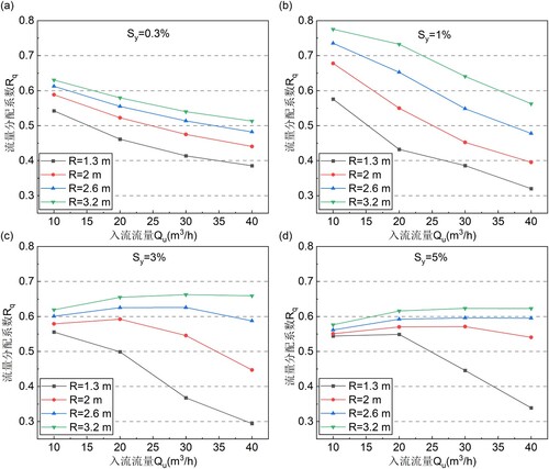
Figure 9. Numerically simulated streamlines at the road crossing under different combinations of turning radius R and longitudeslope S_y.

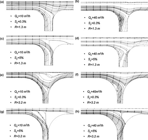
It could be seen from the Figure 8 that, in general, a larger turning radius results a higher flowrate distribution ratio R_q. This result agrees with the fundamental fluid mechanics theory which states that a smooth entrance at the branch channel promotes the flow condition by eliminating separation zones at the entrance. Comparing Figure 9(b) and (f), it could be seen that the size of the separation zone at the entrance of the branch roadway becomes much smaller as the turning radius turns larger. This result also agrees with previous numerical predictions by Shettar and Murthy (1996) on a streamline branch entrance study.

It is also important to point out that in all cases, none of the distribution ratio remains constant. As shown in Figure 8, at different roadway longitude slope S_y condition, the pattern of the distribution ratio (R_q) changing with the inflow flowrate Q_u is quite different. At relatively small longitude slope (S_y=  0.3% and S_y= 1%), the flowrate distribution ratio R_q decreases as inflow Q_u goes up, as shown in Figure 8(a) and (b). This means that in a relatively flat road network, less portion of flood will be diverted into the branch road when high runoff flowrate occurs, for example, in an extreme storm. This is because a high flowrate Q_u results a high momentum in the X direction (main road direction). Flow tends to continue along the main channel due to the high momentum drive. This finding is critical in designing the emergency transportation paths during extreme floods to improve the city’s resilience again natural hazards (Tahvildari et al., 2022). In this way, a proper turning radius could be used at the key junctions to purposely guide the flood into the specified passage instead of into the emergency transportation path. To investigate the reason of this phenomena, flow streamlines were compared in Figure 9(a) and (b). It could be seen that a high flowrate tends to create a separation zone at the entrance of the branch road, especially for small turning radius cases, for example R = 1.3 m. The size of the separation zone is almost 1/2 of the branch roadway width. Due to the separation zone, the flow cross section area is compressed, which reduces the flow capacity and hence the flowrate in the branch road significantly. In the widely used urban stormwater simulation model SWMM, a weir equation is typically used to estimate the flowrate diverted into the branch road (Guo et al., 2021). Results from this study indicates that the contraction coefficient used in the weir equations for a relative flat roadway crossing would be much higher than a steep roadway crossing.

At steep slopes (S_y=  3%, 5%), there are two distinctive trends exist, as shown in Figure 8(c) and (d). For roadways with large turning radius (R = 2.6, 3.2 m), the flow distribution ratio fluctuates little between 0.6 and 0.65 even the upstream flow increases significantly. However, for small turning radius roadways (R = 1.3, 2.0 m) the flow distribution ratio drops rapidly from 0.55 to 0.3 as the inflow flowrate increases. The reason for the reduced flow distribution ratio at small turning radius roadways is similar to what is described above. It is also a result of the high momentum in the X direction (main road direction) under high flowrates. The trend for larger turning radius cases at steep slopes can be explained through flow fields. According to Figure 9 (c) and (d), when longitudinal slope S_y increases to 5%, the recirculation zone of the branch is no longer seen even under a high flowrate. This means the momentum generated by the steep slope could overcome the backwater phenomenon at the branch road, which is the primary cause of a separation zone. In this case, the branch roadway keeps a normal cross area size and the flow capacity varies little. Based on Figure 9(g) and (h), a high elevation spot at the lower right corner of the road crossing could be seen. The high spot was formed because of the compromise of cross slope and longitude slope based on road design specifications (Mohurd, 2011). The high spot blocks the flow in the main road and leads to the flowlines bending towards the branch roadway. As a result, the flow tends to be evenly distributed between the main road and the branch road and is less likely affected by the upstream flowrate. This means that in the design of a steep road crossing, if the flow distribution ratio needs to be kept relatively stable, a turning radius larger than three times of the roadway width will be needed. As steep roads can occur frequently in mountainous cities where the road slope easily reaches 3% or even 5%, results from this study could provide insights into the crossing design to form a more accurate flood transport network.

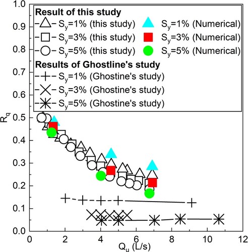
The experimental and numerical results were compared with previous studies on flat bottom diversion channels. In Figure 10, the flow distribution results under free flow boundary conditions were compared with studies by Ghostine et al. (2013) on the flat-bottom channel intersections. A significant difference could be observed. As shown in Figure 10, the flow distribution ratio R_q at a roadway crossing is generally larger than what was observed in the corresponding flat-bottom diversion channel. Furthermore, the discrepancy is more significant when inflow flowrate is low. In addition, the flowrate distribution ratio in the roadway crossing is less affected by the road longitude slope comparing to the diversion channel cases when the roadway slope reaches above 1%. This result is consistent with the fundamental fluid mechanics at a roadway crossing, where the combination of a side slope and turning radius creates acceleration in the transverse direction and pushes the inflow more favorable toward the lateral branch direction.

Figure 10. Comparison of Flowrate distribution ratio from this study and Ghostine’s study on flat-bottom diversion channels (Ghostine et al., 2013).

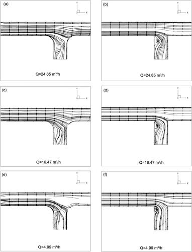
Streamlines of the two configurations are compared in Figure 11. It could be seen that the flow field at the intersection of flat-bottom channels without turning radius shows a noticeable recirculation zone at the entrance of the branch channel. The streamlines are separated from the sidewall due to the abrupt change of the flow direction. The existence of the recirculation zone greatly reduces the effective flow area at the branch channel and leads to a decrease in the flow diversion ratio.

Figure 11. Comparison of streamlines at S_u= S_b= S_d= 1%, (a), (c), (e) are road crossings with side slope and a turning radius of 0.6 m; (b), (d), (f) is the flat bottom diversion channels.

4.3. Influence of roadway longitude slopes

Based on open channel flow theory (Mays, 2005), when Froud number (Fr) of the flow is less than 1.0, the flow field is in a subcritical flow regime and is subject to downstream control. A downstream control means changes in the downstream sides such as longitude slope, turning radius and boundary conditions could affect the flow field at the road crossing. When the Froud number of the flow is larger than 1.0, flow is in a supercritical flow regime and is subject to upstream control in which only the upstream parameters and inflow boundary conditions would impact the flow field at the crossing. In this study, in S_y= 0.3% cases, the upstream Froude number (F_ru) ranges from 0.8 to 0.98 as the flowrate changes from 10 to 40m³/h and the flows are subcritical. In S_y= 3.0% and 5.0%cases, the upstream Froude number (F_ru) changes from 2.89 to 4.11 and the flows are strongly supercritical. In S_y= 1.0% cases, the upstream flows are also supercritical flow but with a low Froude number (F_ru) ranging from 1.41 to 1.81. Because of the different flow regime caused by the longitude slope and the flowrate, the distribution ratio shows different patterns as well.

Through Figure 12 (a) and (b), it could be seen that the influence of longitude slope is not obvious when the turning radius is less than 2.0 m which is about twice of the roadway width. In this case, the distribution ratio increases slightly as longitude slope increases and all the curves are close to each other. This means that at a small turning radius, the turning radius is the dominate factor that influences the distribution ratio. However, when the turning radius reaches 2.6 which is about three times of the roadway width or higher, two groups of trends could be distinguished based on the corresponding slope, as shown in Figure 12(c) and (d). One group is the longitude slope is equal or less than 1%. In these cases, the upstream flow is either in a subcritical dominated regimes (S_y= 0.3% cases) or in a weak supercritical regime (S_y= 1% cases). We could see that the distribution ratio increases with increasing longitude slope. This means in a city with a flat terrain, increasing the road slope could promote more flood into the branch roadway. The other group is the upstream flow field is strongly supercritical (S_y= 3% and 5% cases) in which the distribution ratio decreases with increasing longitude slope. This means less portion of flood would be diverted into the branch road as a result of the increasing longitude slope. Results from this study could help to select the proper parameters in flat cities and mountains cities for flood mitigation purpose against extreme storms.

Figure 12. Relationship of distribution ratio R_q versus inflow flowrate Q_u at different longitude slope S_y when turning radius R is fixed.

4.4. Influence of roadway downstream boundary conditions

In this section, the scenarios where there is standing water at the downstream ends of the road were investigated. Two scenarios were studied. One is standing water present at both main road and branch road downstream sides. The other one is standing water only present at the main road downstream side. For simplification, the road longitude slope of 1.0% was used in all simulations. This is due to the fact that if road longitude gets higher than 1.0%, the flow is more likely in a supercritical condition and less likely to be impacted by the standing water at the downstream side, based on water surface profile theory in open channel flow (Mays, 2005). A relative depth w_d is defined and used to generalize the boundary condition as below: (8) $w_d=\frac{W{D}_{down}}{\mathrm{\Delta }Z}$(8)

Where WD_down is the downstream standing water depth (m), $\mathrm{\Delta }Z$ is elevation drop between the entrance and the outlet of the crossing area (m).

4.4.1. Standing water only present at the main road downstream end

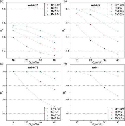
In this case, the standing water only present at the main road downstream while the branch road is still free flow. Four relative depths of standing water W_d ranging from 0.25 to 1.0 were investigated. Figure 13 shows the flowrate distribution ratio at different turning radius R and downstream standing water depth W_d. It could be seen that at a relatively small downstream water depth (W_d  = 0.25), the distribution ratio pattern is very similar to the corresponding case in the free flow boundary condition in Figure 9. It shows that the flowrate distribution ratio increases as the turning radius goes up and drops as the inflow rate goes up. However, as the downstream standing water depth goes higher, the flowrate distribution ratio approaches 1.0 regardless of the turning radius which means almost all the floodwater would be transported into the branch roadway.

Figure 13. Relationship of distribution ratio R_q versus inflow flowrate Q_u at different downstream standing water depth in the main road.

4.4.2. Standing water present at both main road and branch road downstream ends

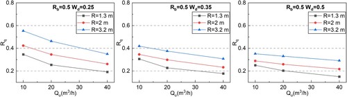
In this case, the standing water present both at the main road downstream and the branch road downstream. Three relative depths of standing water ranging from 0.25 to 0.5 were investigated with four turning radius values were simulated under each depth. Figure 14 shows the flowrate distribution ratio at different turning radius R and downstream standing water depth W_d. It could be seen that at all water depth, the distribution ratio pattern is similar to the corresponding case in the free flow boundary condition in Figure 9. It shows that the flowrate distribution ratio increases as the turning radius goes up and drops as the inflow rate goes up. However, as the downstream standing water depth goes higher, the distribution ratio drops slightly. This means less portion of flow goes into the branch road. It could also be seen that as the standing water depth goes up, the distribution ratio-flowrate curves (R = 1.3, 2, and 3.2 m) tend to flat out and approach to each other. This means the flowrate distribution ratio is less likely impacted by the turning radius and the inflow approaches at high standing water downstream boundary conditions.

Figure 14. Relationship of distribution ratio R_q versus inflow flowrate Q_u at different downstream standing water depth in the main road and branch road.

5 Conclusions

In this study, the flow distribution pattern at a T-shape roadway crossing was studied experimentally and numerically. A physical model of the roadway crossing was established to investigate the flow field as well as provide validation data for the numerical models. The corresponding three-dimensional CFD model was constructed using FLUENT. Results predicted by the numerical model match well with the experimental measurements. A 2^k factorial design test was conducted first to screen the key factors that need to be studied in details. Then detailed numerical studies were conducted to reveal the relationship between the flow distribution ratio and the individual impacting factor include turning radius, longitudinal slope under different flowrates and boundary conditions. Based on the numerical experiment results, the following conclusions could be drawn:

1. Roadway turning radius, roadway longitude slope and upstream flowrate affect the flow distribution ratio at a T-shape crossing significantly. The roadway side slope does not show a strong influence on the flow distribution ratio. In a free flow boundary condition, the combined effect of side slope and turning radius at a road crossing produces a significantly higher flow distribution ratio comparing to a flat bottom diversion channel. The discrepancy is particularly high in low flowrate cases.

2. In general, a larger turning radius results a higher flowrate distribution ratio. At relatively small longitude slope (Sy =  0.3%, 1%) where Froude number is below 1.0 or close to 1.0, the flowrate distribution ratio decreases with increasing inflow flowrate regardless of the turning radius. At steep slopes (S_y=  3% and S_y= 5%), flow distribution ratio varies little with increasing inflow flowrate in a large turning radius configuration, while flow distribution ratio drops significantly in a small turning radius configuration.

3. At a small turning radius (less than twice of the roadway width), the influence from the longitude slope is not obvious and the turning radius is the dominate factor that influences the distribution ratio. At a large turning radius, if the flow is in a subcritical dominated state or a weak supercritical state, the distribution ratio increases with increasing longitude slope. At a large turning radius, the distribution ratio decreases with increasing longitude slope if the upstream flow field is in a strong supercritical state.

4. In cases where there is standing water at downstream ends, the flow distribution ratio is almost not affected by the downstream water but by the turning radius when the relative water depth is lower than 0.25. If the standing water is at the main road downstream side, the flow distribution ratio approaches to 1.0 regardless of the turning radius as the relative water depth rises. When there are standing water on both main and branch road downstream sides, impacts from turning radius and longitude slopes diminishes as the relative water depth rises.

In this study, the flow distribution ratio at a roadway crossing with a T-shape was investigated. To our knowledge, this is the first attempt to study the flow distribution pattern at a road crossing. Findings from this research could provide more accurate flowrate predictions for the downstream roads and hence improve the safety of a major drainage system during extreme storms. This research work could also help designing the emergency transportation paths during extreme floods to improve the city’s resilience again natural hazards. However, due to time limits, the influence caused by different roadway width from the main road and the branch road did not cover while it could affect the flow distribution ratio significantly. The transition of flow regimes caused by different upstream and downstream longitude slope is not investigated neither. These additional configurations could be investigated in the future studies.

Acknowledgement

We acknowledge the financial support of National Natural Science Foundation of China (NSFC) General Program (grant number 52070027).

Disclosure statement

No potential conflict of interest was reported by the author(s).

Additional information

Funding

This work was supported by National Natural Science Foundation of China (NSFC) [Grant Number: 52070027].

References

- Abderrezzak, K. E. K., Lewicki, L., Paquier, A., Riviere, N., & Travin, G. (2011). Division of critical flow at three-branch open-channel intersection. Journal of Hydraulic Research, 49(2), 231–238. https://doi.org/10.1080/00221686.2011.558174
- Azimi, H., & Shabanlou, S. (2015). The flow pattern in triangular channels along the side weir for subcritical flow regime. Flow Measurement and Instrumentation, 46, 170–178. https://doi.org/10.1016/j.flowmeasinst.2015.04.003
- Chang, T. J., Wang, C. H., Chen, A. S., & Djordjevic, S. (2018). The effect of inclusion of inlets in dual drainage modelling. Journal of Hydrology, 559, 541–555. https://doi.org/10.1016/j.jhydrol.2018.01.066
- Fluent, A. (2018). Version 19.0. ANSYS Inc.
- Ghostine, R., Vazquez, J., Terfous, A., Riviere, N., Ghenaim, A., & Mose, R. (2013). A comparative study of 1D and two-dimensional approaches for simulating flows at right angled dividing junctions. Applied Mathematics and Computation, 219(10), 5070–5082. https://doi.org/10.1016/j.amc.2012.11.048
- Guo, K., Guan, M., & Yu, D. (2021). Urban surface water flood modelling – a comprehensive review of current models and future challenges. Hydrology and Earth System Sciences, 25(5), 2843–2860. https://doi.org/10.5194/hess-25-2843-2021
- Hsu, C. C., Tang, C. J., Lee, W. J., & Shieh, M. Y. (2002). Subcritical 90 degrees equal-width open-channel dividing flow. Journal of Hydraulic Engineering, 128(7), 716–720. https://doi.org/10.1061/(asce)0733-9429(2002)128:7(716)
- Huang, J., Weber, L. J., & Lai, Y. G. (2002). Three-dimensional numerical study of flows in open-channel junctions. Journal of Hydraulic Engineering, 128(3), 268–280. https://doi.org/10.1061/(ASCE)0733-9429(2002)128:3(268)
- Kesserwani, G., Vazquez, J., Riviere, N., Liang, Q., Travin, G., & Mose, R. (2010). New approach for predicting flow bifurcation at right-angled open-channel junction. Journal of Hydraulic Engineering, 136(9), 662–668. https://doi.org/10.1061/(asce)hy.1943-7900.0000222
- Kourtis, I. M., & Tsihrintzis, V. A. (2021). Adaptation of urban drainage networks to climate change: A review. Science of the Total Environment, 771, 145431. https://doi.org/10.1016/j.scitotenv.2021.145431
- Li, C., & Zeng, C. (2009). Three-dimensional numerical modelling of flow divisions at open channel junctions with or without vegetation. Advances in Water Resources, 32(1), 49–60. https://doi.org/10.1016/j.advwatres.2008.09.005
- Li, X., Erpicum, S., Mignot, E., Archambeau, P., Pirotton, M., & Dewals, B. (2021). Influence of urban forms on long-duration urban flooding: Laboratory experiments and computational analysis. Journal of Hydrology, 603 (127034),1-16, https://doi.org/10.1016/j.jhydrol.2021.127034
- Mays, L. W. (2005). Water resources engineering (2nd Edition). John Wiley & Sons Inc.
- Mignot, E., Li, X., & Dewals, B. (2019). Experimental modelling of urban flooding: A review. Journal of Hydrology, 568, 334–342. https://doi.org/10.1016/j.jhydrol.2018.11.001
- Mizumura, K., Yamasaka, M., & Adachi, J. (2003). Side outflow from supercritical channel flow. Journal of Hydraulic Engineering, 129(10), 769–776. https://doi.org/10.1061/(asce)0733-9429(2003)129:10(769)
- Mohurd(Ministry of Housing and Urban-Rural Developemnt). (2011). Code for design of urban road traffic facility (GB 50688-2011). Beijing China Planning Press.
- Momplot, A., Kouyi, G. L., Mignot, E., Riviere, N., & Bertrand-Krajewski, J. L. (2017). Typology of the flow structures in dividing open channel flows. Journal of Hydraulic Research, 55(1), 63–71. https://doi.org/10.1080/00221686.2016.121-2409
- Montgomery, D. C. (2005). Design and analysis of experiments (6th Edition). John Wiley & Sons Inc.
- Nania, L. S., Gomez, M., & Dolz, J. (2004). Experimental study of the dividing flow in steep street crossings. Journal of Hydraulic Research, 42(4), 406–412. https://doi.org/10.1080/00221686.2004.9641208
- Neary, V. S., & Odgaard, A. J. (1993). Three-dimensional flow structure at open-channel diversions. Journal of Hydraulic Engineering, 119(11), 1223. https://doi.org/10.1061/(ASCE)0733-9429(1995)121:1(87)
- Ramamurthy, A. S., Qu, J., & Vo, D. (2007). Numerical and experimental study of dividing open-channel flows. Journal of Hydraulic Engineering, 133(10), 1135–1144. https://doi.org/10.1061/(asce)0733-9429(2007)133:10(1135)
- Ramamurthy, A. S., & Satish, M. G. (1988). Division of flow in short open channel branches. Journal of Hydraulic Engineering, 114(4), 428–438. https://doi.org/10.1061/(asce)0733-9429(1988)114:4(428)
- Ramamurthy, A. S., Tran, D. M., & Carballada, L. B. (1990). Dividing flow in open channels. Journal of Hydraulic Engineering, 116(3), 449–455. https://doi.org/10.1061/(asce)0733-9429(1990)116:3(449)
- Riviere, N., Perkins, R. J., Chocat, B., & Lecus, A. (2006). Flooding flows in city crossroads: Experiments and 1-D modelling. Water Science and Technology, 54(6-7), 75–82. https://doi.org/10.2166/wst.2006.603
- Rivière, N., Travin, G., & Perkins, R. J. (2014). Transcritical flows in three and four branch open-channel intersections. Journal of Hydraulic Engineering, 140(4), 4. https://doi.org/10.1061/(asce)hy.1943-7900.0000835
- Schmitt, T. G., Thomas, M., & Ettrich, N. (2004). Analysis and modeling of flooding in urban drainage systems. Journal of Hydrology, 299(3-4), 300–311. https://doi.org/10.1016/j.jhydrol.2004.08.012
- Shams, A., Sarasua, W. A., Putman, B. J., Davis, W. J., & Ogle, J. H. (2020). Highway cross-sectional design and maintenance to minimize hydroplaning. Journal of Transportation Engineering Part B: Pavements, 146(4), 04020065. https://doi.org/10.1061/JPEODX.0000213
- Sharifipour, M., Bonakdari, H., Zaji, A. H., & Shamshirband, S. (2015). Numerical investigation of flow field and flowmeter accuracy in open-channel junctions. Engineering Applications of Computational Fluid Mechanics, 9(1), 280–290. https://doi.org/10.1080/19942060.2015.1008963
- Shettar, A. S., & Murthy, K. K. (1996). A numerical study of division of flow in open channels. Journal of Hydraulic Research, 34(5), 651–675. https://doi.org/10.1080/0022168960949-8464
- Tahvildari, N., Abi Aad, M., Sahu, A., Shen, Y., Morsy, M., Murray-Tuite, P., Goodall, J. L., Heaslip, K., & Cetin, M. (2022). Quantification of compound flooding over roadway network during extreme events for planning emergency operations. Natural Hazards Review, 23(2), 04021067. https://doi.org/10.1061/(ASCE)NH.1527-6996.0000524
- Tellman, B., Sullivan, J. A., Kuhn, C., Kettner, A. J., Doyle, C. S., Brakenridge, G. R., Erickson, T. A., & Slayback, D. A. (2021). Satellite imaging reveals increased proportion of population exposed to floods. Nature, 596(7870), 80–86. https://doi.org/10.1038/s41586-021-03695-w
- White, F. M., & Island, U. (2011). Fluid mechanics. McGraw-Hill Education.
- Younus, M., & Hanif Chaudhry, M. (1994). A depth-averaged turbulence model for the computation of free-surface flow. Journal of Hydraulic Research, 32(3), 415–444. https://doi.org/10.1080/00221689409498744