Numerical study of the fire-smoke temperature law in the shaft of a high-rise building under the chimney effect in winter

Abstract

Shaft structures in high-rise buildings may increase fire coverage due to chimney effects. However, few previous studies have considered the motion of the flue gas under the combined effect of the chimney effect and thermal buoyancy. So, we set a continuous gradient differential pressure opening based on the characteristics of the chimney effect in winter. The CFD method is used to simulate 12 operating conditions with different fire source locations and rates of heat release from the ignition source. We compare and analyze the temperature rise, the flue gas rise law and the variation of the thermal pressure difference between the inner and outer shafts for different fire source powers. The results show that, in the case of low-floor fires, the range of temperature appreciation and fluctuation at the local measurement point increases with the fire power and the distribution of temperature appreciation decreases with the height. The relationship between the dimensionless time and the dimensionless height of the flue gas layer is exponential for different fire position conditions. The fire causes the neutral surface to shift, and below the original neutral surface, the higher the position of the fire source, the more pronounced the shift of the neutral surface.

KEYWORDS:

• Chimney effect
• numerical simulation
• shaft
• flue gas movement
• neutral surface

1. Introduction

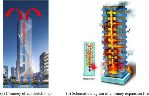
In recent years, with the acceleration of urbanization, high-rise buildings emerge in an endless stream. There are many vertical shaft structures in high-rise buildings, such as shared atriums, vertical ventilation or smoke exhaust air ducts, stairwells and so on. Especially in winter in the northern region where the temperature difference between indoor and outdoor is large, there is a large pressure difference between the inside and outside of the shaft. The cold air penetrates into the shaft through building gaps such as in doors, windows and curtain walls, forming a chimney effect, as shown in Figure 1(a). The chimney effect will lead to a series of problems, such as building elevator failure, aerodynamic noise and high energy consumption problems, especially in the case of a building fire. The chimney effect will make the smoke in the elevator shaft spread vertically rapidly, then through the lateral openings of the floor above the neutral surface there will be horizontal spread, resulting in fire smoke spreading to unburned areas, causing greater difficulty for personnel evacuation, as shown in Figure 1(b).

Figure 1. Winter chimney effect in high-rise buildings: (a) chimney effect sketch map; (b) schematic diagram of chimney expansion fire.

Previous studies on the chimney effect mainly focused on the neutral plane position of the whole building (Mao, 2012; Yin, 2015) and how to suppress the chimney effect (Lu et al., 2018; Shi et al., 2014; Wu, 2018; Xie & Huang, 2019). Ji et al. (2013) and Li et al. (2014) conducted a series of combustion tests in a one-third scale stairwell to study how long it took the front end of the buoyancy plume to reach a certain height from the fire source in a stairwell with the top vent open and closed. The relation between the dimensionless rise time and the dimensionless rise height of the stairwell has been proposed to predict the rise time of the plume front. Based on the KLOTE model (Klote, 1993), Xu et al. (2011) established a continuous model for predicting the height of the neutral surface of the shaft in case of fire according to the characteristics of continuous distribution of temperature in the shaft. They also compared the KLOTE model, the two-region model and the continuous model with the simulation results, and confirmed that the continuous model had the least deviation.

Li (2018) studied the fire development mechanism in high-rise buildings under the action of multiple factors such as fire source power, the chimney effect, and external wind, and the control of smoke flow by positive pressure air supply measures, using theoretical analysis, a tiny-scale test, numerical simulation and other research methods. The effects of the chimney effect on the dynamic balance of a fire plume in the fire space in the early stage of high-rise building fire and the effects of reverse wind on the combustion characteristics of a double-opening mouth chamber in the intense development stage of a high-rise building fire were studied by small-scale experiments. Zhu et al. (2020) studied the influence of external crosswinds on air flow behaviour, methanol tank combustion characteristics, and flue gas temperature in a vertical shaft corridor.

A series of experiments with different fire sources and opening locations in a 21-floor office building were carried out by He et al. (2020; 2022) to study the transmission and stratification of hot smoke in the stairwell. It was found that the intensity of the chimney effect in stairwells first increases and then decreases with increasing opening height, and a comprehensive correlation formula was proposed to predict the rise time of the flue gas plume in stairwells. In addition, large eddy simulations were used to model the smoke flow in a full-size stairwell, and the effects of environmental pressure and heat release rate on the smoke flow were studied. An air mass flow prediction equation including the ambient pressure and the heat release rate of the fire source was proposed. At the same time, an empirical model for the prediction of the plume rise time taking into account the environmental pressure was presented. Sun et al.(2009) studied smoke movement in a stairwell of six floors caused by a fire in adjacent compartments, observed the smoke flow law in the stairwell, and measured the distribution of the vertical temperature field and velocity field. The smoke flow was observed to move upward in a circular pattern and to form vortices below the treads of the stairwell on each floor, with the stairwell smoke temperature generally decreasing exponentially with height.

At present, the chimney effect and its effect on high-rise building fires have been studied to some extent. However, less attention has been paid to fires in elevator shafts, and fire sources have mostly been located on the bottom floor; fires situated on other floors have been studied less. In addition, the chimney effect and thermal buoyancy are common in the occurrence of fires, but they have rarely been considered together. Therefore, different fire source locations and various fire source power conditions are considered for a building elevator shaft in this article. A two-dimensional numerical simulation method is adopted to study the transient changes in the local temperature rise and smoke movement rule in the shaft under the chimney effect, as well as changes in the thermal pressure difference inside and outside the shaft.

The innovation of this article is to pay attention to the temperature variation law and flue gas flow characteristics in a shaft structure under the combined action of flue gas buoyancy and the chimney effect, and to analyse the influence of different ignition powers and different ignition locations on the flue gas temperature law.

2. Physical modes and numerical method

2.1. Shaft model and monitoring points

In view of elongated vertical shafts in high-rise buildings, and the research focus being on the vertical rising law of flue gas, the physical model of this article is a two-dimensional elevator shaft in a high-rise building. Figure 2(a) shows the calculation model for the shaft. There is no elevator in the shaft. The width b is 2.4 m and the height h is 52.5 m. When a fire breaks out in a building, smoke typically enters the shaft structure through a crack in the elevator door and then diffuses through the building shaft under the chimney effect. An opening is set at the top of the shaft, with a size of 240 mm, which is converted according to the proportion of the opening area at the top of the shaft to the top surface, as shown in Figure 2(b). The opening of the elevator door seam is set at the position of the elevator door on each floor. The height is 33 mm, which is converted according to the proportion of the area of the elevator door seam on each floor to the wall, as shown in Figure 2(c). The boundary condition of the top opening of the model is pressure-outlets, the opening of the door is pressure-inlets, and other boundaries are wall boundaries.

Figure 2. Schematic diagram of the computational model.

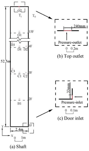
The ambient temperature of the model is set according to the extreme weather in North China in winter. The ambient temperature T₀ is −15°C, and the temperature T_i in the shaft is 20°C. According to the theoretical calculation formula for indoor and outdoor thermal pressure difference under the chimney effect in the ASHRAE Handbook (ASHRAE, 2009), the pressure difference at the opening of door cracks of each layer can be obtained, and the calculation formula is as follows: (1) $\begin{array}{r}\mathrm{\Delta }{P}_s=3465\left(\frac{1}{T_o}-\frac{1}{T_i}\right)(H_{\text{NPL}}-H)\end{array}$(1) where ΔP_s is the difference between the indoor and outdoor pressures, T_i and T₀ are the absolute indoor and outdoor temperatures, respectively, H_NPL is the height of the medium and horizontal plane (this article defaults to 1/2 of the shaft), and H is the calculated height of the shaft.

According to the temperature characteristics of the shaft structure, the monitoring points are shown in Figure 2, and the coordinates of the monitoring points are shown in Table 1. According to the research content, six different fire power sources and two different fire source positions are set, which are located at the opening position of the door seams on the first floor and the fifth floor, respectively. Setting the heat source in the temperature gradient region promotes heat exchange (Cheng et al., 2021). All working conditions are shown in Table 2.

Table 1. Monitoring point information.

	Coordinates
Point	x (m)	y (m)
B1	1.20	3.5
F1	1.20	17.5
J1	1.20	31.5
O2	1.20	52.3
C2	2.28	8.2
C3	0.12	9.4
D2	2.28	8.2
D3	0.12	9.4

Table 2. Working condition list.

Case name	Heat release rate of fire source (MW)	Symbol	Case name	Heat release rate of fire source (MW)	Symbol
QL1	1.0		QM1	1.0
QL2	1.5		QM2	1.5
QL3	2.5		QM3	2.5
QL4	3.0		QM4	3.0
QL5	4.0		QM5	4.0
QL6	5.0		QM6	5.0

Note: L is for fire on the first floor of the shaft, M is for fire on the fifth floor of the shaft.

2.2. Numerical method

In this article, the governing equations of the standard k–ε model are adopted. The continuity equation is (2) $\begin{array}{r}\mathrm{div}(\rho U)=0\end{array}$(2)

The momentum equations are (3) $\begin{array}{rl}\frac{\mathrm{\partial }(\rho u)}{\mathrm{\partial }{t}^{\mathrm{\prime }}}+\mathrm{div}(\rho uU)& =\mathrm{div}(\mu gradu)-\frac{\mathrm{\partial }p}{\mathrm{\partial }x}\end{array}$(3) (4) $\begin{array}{rl}\frac{\mathrm{\partial }(\rho v)}{\mathrm{\partial }{t}^{\mathrm{\prime }}}+\mathrm{div}(\rho vU)& =\mathrm{div}(\mu gradv)-\frac{\mathrm{\partial }p}{\mathrm{\partial }y}\end{array}$(4)

The energy equation is (5) $\begin{array}{r}\frac{\mathrm{\partial }(\rho T)}{\mathrm{\partial }{t}^{\mathrm{\prime }}}+\mathrm{div}(\rho UT)=\mathrm{div}\left(\frac{k}{c_p}\mathrm{grad}T\right)+S_T\end{array}$(5)

The transport equations corresponding to turbulent kinetic energy k and turbulent dissipation rate ε are shown in Equations (6) and (7). (6) $\begin{array}{rl}\frac{\mathrm{\partial }(\rho k)}{\mathrm{\partial }{t}^{\mathrm{\prime }}}+\frac{\mathrm{\partial }(\rho k{u}_i)}{\mathrm{\partial }{x}_i}& =\frac{\mathrm{\partial }}{\mathrm{\partial }{x}_i}\left[\left(\mu +\frac{{\mu }_i}{{\sigma }_k}\right)\frac{\mathrm{\partial }k}{\mathrm{\partial }{x}_j}\right]\\ & +G_k+G_b-\rho \epsilon \end{array}$(6) (7) $\begin{array}{rl}\frac{\mathrm{\partial }(\rho \epsilon )}{\mathrm{\partial }{t}^{\mathrm{\prime }}}+\frac{\mathrm{\partial }(\rho \epsilon u_i)}{\mathrm{\partial }{x}_i}& =\frac{\mathrm{\partial }}{\mathrm{\partial }{x}_i}\left[\left(\mu +\frac{{\mu }_i}{{\sigma }_{\epsilon }}\right)\frac{\mathrm{\partial }\epsilon }{\mathrm{\partial }{x}_j}\right]\\ & +C_{1\epsilon }\frac{\epsilon }{k}(G_k+C_{3\epsilon }{G}_b)-C_{2\epsilon }\rho \frac{{\epsilon }_2}{k}\end{array}$(7) where ρ is the density of air, t′ is the time, U is the velocity vector, u and v are the components of U in the x- and y-directions of the coordinate system, respectively, μ is the aerodynamic viscosity, S_T is the internal heat source of fluid and fluid mechanical energy into heat energy due to the viscous action part, G_k is the production term of the turbulent kinetic energy k due to the average velocity gradient, G_b is the generation term of the turbulent kinetic energy k due to buoyancy, C_1ε, C_2ε, and C_3ε are empirical constants, and σ_k and σ_ε are Prandtl numbers corresponding to the turbulent kinetic energy k and the dissipation rate ε, respectively (Zhang, 2011).

The governing equations are discretized by the finite volume method. The convection term is discretized by a second-order upwind scheme, the diffusion term is discretized by a second-order central difference scheme, and the time term is discretized by a second-order implicit scheme. The Semi-Implicit Method for Pressure Linked Equations (SIMPLE) algorithm is used to solve the governing equation by pressure and velocity coupling. The coupled heat transfer model is an effective tool in the study of heat transfer problems (Xie et al., 2021).

2.3. Grid and calculation validity verification

A structured grid is adopted in the computing domain of the model, as shown in Figure 3. The grid is encrypted in the boundary layer and the opening, and the y⁺ value is 100.

Figure 3. Schematic diagram of shaft model mesh: (i) is the mesh near the top outlet, and (ii) is the mesh near the bottom entrance. (a) whole grid; (b) 1st local grid; (c) grid near boundary.

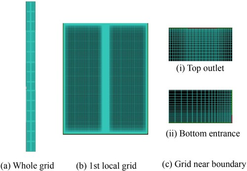
A grid independence test, a time step independence test, and a turbulence model test are carried out in the early stage of calculation. In this article, the Q_L1 working condition is taken as an example to detect the four grid quantities

1.8 × 10⁵, 4.2 × 10⁵, 6.2 × 10⁵, and 8.6 × 10⁵. The mean values of temperature at measuring points in the fully developed stage are shown in Table 3. Based on the second grid, the mean values of the temperature measurement points at the full development stage are compared. It can be seen that there is some difference between grid 1 and grid 2, with a maximum relative error of 3.05%, while grid 3 and grid 4 are within 1% of grid 2. Therefore, in order to obtain accurate simulation results with limited computational resources and time, the second grid scheme is chosen for the calculations. In the verification of time step independence, four different sets of time steps are given in Table 4, namely 0.005, 0.010, 0.040, and 0.080 s. The temporal mean of the temperature at the monitoring point during the fully developed phase is compared based on operating conditions with a time step of 0.040 s. The relative errors are large. When the time step is less than 0.04 s, the relative error is less than 0.5%. So 0.04 s is chosen as the time step for the calculation.

Table 3. Grid independence verification.

			Relative error of average temperature at measuring point
Number	Grid distribution	Quantity	C3 (%)	C2 (%)	D3 (%)	D2 (%)
1	115 × 1590	1.8$\times$10^5	0.80	1.90	1.33	3.05
2	184 × 2295	4.2$\times$10^5	—	—	—	—
3	245 × 2530	6.2$\times$10^5	0.17	0.46	0.22	0.80
4	303 × 2835	8.6$\times$10^5	0.37	0.75	0.40	0.88

Table 4. Time step independence verification.

		Relative error of average temperature at measuring point
Number	Time step (s)	C3 (%)	C2 (%)	D3 (%)	D2 (%)
1	0.005	0.04	0.02	0.02	0.03
2	0.010	0.06	0.01	0.01	0.02
3	0.040	—	—	—	—
4	0.080	0.32	0.35	0.11	0.22

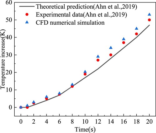
In order to verify the applicability of the turbulence model to this problem, the numerical calculation of the fire source condition at the bottom of the three-dimensional shaft is carried out, and the mutual verification is made with the experimental data and theoretical prediction results in the literature (Ahn et al., 2019). Figure 4 shows a comparison of the temperature data at the measuring point at 9 m height. For reference, the t²-ignition source is used at the beginning, so the power of the ignition source can also be mentioned at the beginning. In the validation of the turbulence model in this article, the same model and boundary conditions as in Ahn et al. (2019) are set up to recover the simulation process fully. At the same time, the agreement at early times is better compared to the data from theoretical studies. At later times, the heat exchange between the fire source and the building is not taken into account in the numerical simulations and is therefore slightly larger, but the relative error is kept within 10%. Therefore, the adopted numerical method is plausible. In addition, there is literature (Sergio et al., 2011) to evaluate three buoyancy correction turbulence models of thermal buoyancy plume, namely the k–ω model, the standard k–ε model, and the RNG k–ε model, indicating that the standard k–ε model has superior accuracy in the study of this problem.

Figure 4. Comparison of CFD simulation, theoretical prediction and experimental data (Ahn et al., 2019).

2.4. Dimensionless parameter definition

In order to characterize the temperature variation rule in the shaft better, the dimensionless temperature rise θ is introduced in this article: (8) $\begin{array}{r}\theta =(T-T_i)/T_i\end{array}$(8) where T is the temperature at the measuring point and T_i is the temperature in the shaft.

Predecessors conducted fire tests on shafts of different sizes, and found that the relationship between t required for smoke rising height z and fire power Q is as follows (Tanaka et al., 2000): (9) $\begin{array}{r}t\propto Q^{1/3}{\int }_0^z{\left(\frac{A}{z}\right)}^{1/3}\text{d}z\end{array}$(9) where Q is the power of the fire source (kW), A is the cross-sectional area of the ascending channel (m²), and z (m) is the ascending height of the smoke (i.e. the distance between the flue gas in the vertical channel and the fire source). On this basis, Tanaka et al. (2000) proposed a more widely used dimensionless rise time τ : (10) $\begin{array}{r}\tau =t\sqrt{\frac{g}{D}}{\left[\frac{Q}{C_p\rho T_0\sqrt{g}{D}^{2.5}}\right]}^{1/3}\end{array}$(10) where g is the acceleration due to gravity, D is the characteristic scale (in this article, the height of a floor is 3.5 m), and C_p is the isobaric specific heat capacity of air.

The dimensionless height Z of smoke rising is defined as (11) $\begin{array}{r}Z=z/D\end{array}$(11)

3. Result analysis

3.1. Transient development temperature rise law in shaft under low floor fire conditions

Figure 5 shows the variation curve of dimensionless temperature rise with dimensionless time at the monitoring point on the central axis of the shaft under low floor fire conditions. The coordinates of each measuring point are shown in Table 1; measuring point B1 is located near the fire source, measuring points F1 and J1 are located in the middle of the shaft, and measuring point O2 is located near the top opening of the shaft. The temperature rise of the selected measuring point can reflect the overall temperature rise change in the shaft. As can be seen from the temperature rise time series at each measuring point under different fire powers in Figure 5, the temperature rise enters the full development stage after undergoing the initial and evolutionary stages, the time for the temperature rise to reach the full development stage is longer with increasing fire power, and the temperature rise increases with increasing fire power.

Figure 5. Dimensionless temperature rise curves of monitoring points B1, F1, J1, and O2 over time for low-floor fire cases: (a) B1; (b) F1; (c) J1; (d) O2.

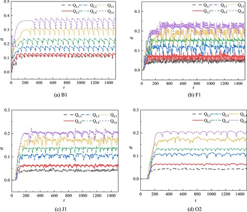
As can be seen from the temperature rise time series of each measuring point under different fire powers in Figure 5, the temperature rise enters the full development stage after undergoing the initial and evolutionary stages, and the time for the temperature rise to reach the full development stage is longer with increasing fire power, and the temperature rise increases with increase fire power. In Figure 5(a), the dimensionless temperature rise of Q_L1∼Q_L6 at measuring point B1 fluctuates around 0.1, 0.12, 0.16, 0.21, 0.28, and 0.35, respectively. With increasing fire power, the temperature rise at this measuring point is higher and the fluctuation is more severe.

By comparing the temperature rise at different positions in the shaft in Figures 5(a)∼5(d), the temperature rise of the measuring points in the fully developed stage shows periodic or quasi-periodic oscillation, which is obvious at the position close to the fire source. In a certain area, with increasing distance from the fire source, the temperature appreciation at the measuring point decreases significantly. When the height exceeds J1, the temperature appreciation at each monitoring point shows little change. For example, the temperature appreciation of B1, F1, J1, and O2 in the Q_L1 working condition is about 0.11, 0.04, 0.04, and 0.04, respectively.

It can be seen from the temperature rise changes at the monitoring points in Figure 5 that the temperature rise at some monitoring points presents periodic changes. In order to obtain the flow period and amplitude changes, power spectrum analysis is carried out on the dimensionless temperature rise at measuring points B1, F1, J1, and O2, as shown in Figure 6. There is a clear master frequency in the temperature rise power spectrum at measuring point B1 under each working condition, and the master frequencies in Q_L1∼Q_L6 is f₁= 0.0193, f₂= 0.0170, f₃= 0.0117, f₄= 0.0096, f₅= 0.0083, f₆= 0.0075, respectively. The master frequency decreases with increasing fire power. The higher the power of the bottom fire source, the more complex is the temperature field near the bottom of the shaft and the more violent the flow oscillation.

Figure 6. Dimensionless temperature rise spectrum analysis of monitoring points B1, F1, J1, and O2 for low-floor fire cases: (a) B1; (b) F1; (c) J1; (d) O2.

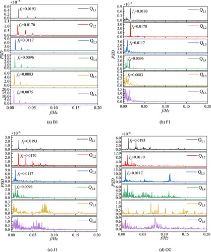
Comparing Figures 6(a)∼6(d) (reflecting the temperature rise frequency distribution in the whole shaft area), it can be seen that the main frequency of the temperature rise spectrum in the whole range does not change with height for cases before Q_L3 (the heat release rate of the fire source is less than 2.5 MW), indicating that the heat release rate of the fire source is the main influencing factor. Among them, there are different degrees of harmonic frequency multiplication with increasing height. It can be seen that, except for the influence of the bottom fire source, the influence of the inlet pressure at other layers on the temperature in the shaft gradually increases with increasing height.

In Q_L4 and later cases (ignition power greater than or equal to 3 MW), there is a clear master frequency below the height of measuring point F1 in the shaft, and the heat release rate of the fire source is the main influencing factor. There is no longer a clear master frequency above the height of F1 measuring point. When the height of the measuring point in the shaft is greater than F1, the flow presents weak turbulent characteristics, and both the bottom fire source and the external cold air intrusion have a great influence on the flow field and temperature field in this region.

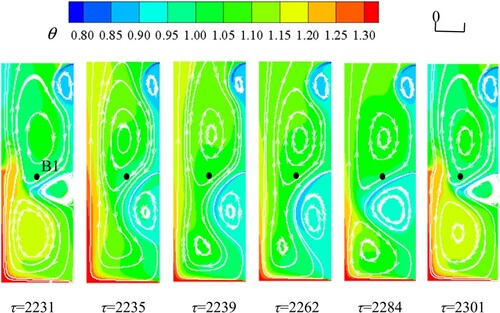
Figures 5 and 6 show the periodic characteristics of the flow from the perspective of time. In order to display the changes of the flow structure near the fire source in the shaft more visually in the spatial dimension, Figure 7 shows the series curve of temperature rise in one cycle at measuring point B1 in the fully development stage for case Q_L3, the red dots represent six selected moments, and Figure 8 is the temperature cloud map corresponding to these moments at measuring point B1. It can be seen that, in one period (τ = 2231∼2301), the heat flow invades from the bottom door seam, forming a rising plume along the left wall, forming a clockwise vortex near the left wall, and cold flow invades near entrance B1, forming a counterclockwise vortex under the entrance. The motion of the hot and cold plumes in the building shaft is similar to the flow in the attic (Cui et al., 2022). In one period, momentum and energy exchange occur in the vortex structure, the hot and cold plume fluctuates, and the temperature oscillates at the measuring point in the centerline. The flow and temperature structure in the second floor is similar to that in the first floor, but the vortex energy is obviously weakened.

Figure 7. Time series of temperature rise at monitoring point B1 in the fully developed phase for case Q_L3.

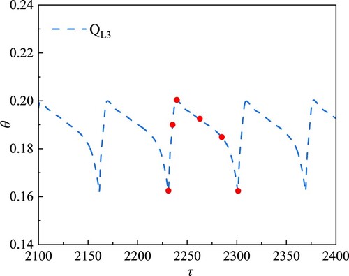
Figure 8. Temperature rise contour and streamline near the point B1 for case Q_L3.

3.2. Temperature rise distribution in the shaft

Figure 9 shows the change of dimensionless temperature rise θ of different fire powers with the rise of flue gas dimensionless height Z, which can be expressed by the exponential function θ (Z) (Ji et al., 2013): (12) $\begin{array}{r}\theta (Z)=\frac{\alpha e^{-\beta ZD}}{T_i}\end{array}$(12)

Figure 9. Temperature rise at different heights in the shaft.

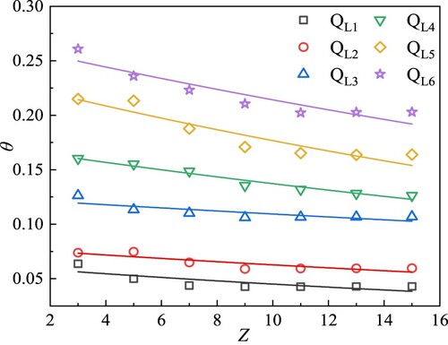
According to the dimensionless temperature rise curve, the approximate temperature distribution T_s at different positions in the shaft under different fire power sources can be obtained: (13) $\begin{array}{r}{T}_s(Z)=T_i+T_i\theta (Z)\end{array}$(13)

Since the area near the fire source is greatly affected by the fire source, only the area with Z > 3 is studied in this article. Table 5 shows the fitting parameters and correlation coefficients. It can be seen that the temperature rise distribution in the shaft decreases exponentially with height. In the simulated fire cases, the coefficient β is about 0.01, and the coefficient α increases from 0.065 to 0.245 with increasing power of the fire source. The heat release rate of the fire source increases from 1.0 to 5.0 MW, and the temperature rise range increased from 0.05 to 0.25. The higher the power of the fire source, the greater is the overall temperature rise; the smaller the power of the fire source, the more uniform is the temperature distribution of the flue gas in each layer of the shaft, and the average dimensionless temperature rise above the 8th floor is basically unchanged.

Table 5. Fitting parameters and correlation coefficients.

Case	α	β
QL1	0.065	0.011
QL2	0.096	0.013
QL3	0.145	0.008
QL4	0.168	0.012
QL5	0.231	0.009
QL6	0.245	0.009

3.3. Smoke rise Law in the shaft

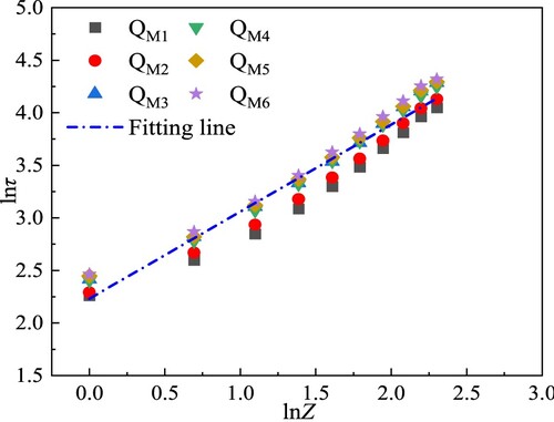
Figures 10 and 11, respectively show the relationship between τ and Z of the fire smoke rise time in the low and middle floors, and the following relationship can be obtained by fitting (Li, 2014; Zhang et al., 2006): (14) $\begin{array}{r}\ln \tau =a+b\ln Z\end{array}$(14)

Figure 10. Relationship between smoke rise time and rise height for low-floor fire cases.

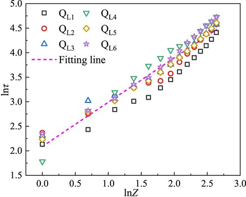
Figure 11. Relationship between smoke rise time and rise height for middle-floor fire cases.

After linear fitting of each working condition of low-floor fire, the relationship is as follows: (15) $\begin{array}{r}\ln \tau =2.088+0.903\ln Z\end{array}$(15)

The expression for the dimensionless time against dimensionless plume rise height are obtained as follows: (16) $\begin{array}{r}\tau =8.069Z^{0.903}\end{array}$(16)

By using the same research method, the smoke rising time law in the shaft when the middle floor is on fire can be obtained as follows: (17) $\begin{array}{r}\ln \tau =2.232+0.827\ln Z\end{array}$(17)

The dimensionless time against dimensionless plume rise height can be expressed as (18) $\begin{array}{r}\tau =9.312Z^{0.827}\end{array}$(18)

Figure 12 shows a comparison between the smoke rise law in this article and the smoke rise law without considering the chimney effect. In the literature, the law of smoke rise in the closed shaft studied by Zhang (2016), the expression is $\tau =3.240Z^{1.500}$. As can be seen from the figure, when a fire occurs on a low floor, the plume rising speed in the area near the fire source in the shaft is slower than that in a closed shaft, which is due to the chimney effect caused by the environmental temperature difference. The low floor draws in the cold air from outside significantly, cooling the hot smoke in the area near the fire source, and transverse cold air enters the shaft and mixes with the rising hot smoke air, resulting in a complex plume spreading path. Changing the short vertical path up the side wall of the shaft, therefore, the plume rise in the shaft is slower than that in a closed shaft when Z < 4.609. When the hot gas rises to a certain height, the transverse gradient pressure difference decreases, and the vertical pulling force and thermal buoyancy generated by the chimney effect play a major role, which makes the plume rise faster in a vertical shaft than in a closed shaft in the area where Z > 4.609. When a fire occurs on the middle floor, the smoke rising law is generally consistent with that of the lower floor. However, with increasing non-scale height, the plume rising speed at the middle floor is slightly faster than that at the lower floor, which gradually becomes obvious after Z > 12. This is because, when the height of the shaft is fixed, the shorter the distance travelled by the heat plume, the less is the heat loss, and the greater the effect of thermal buoyancy. Therefore, for a fire on the middle floor, the smoke rises faster in the area where Z > 12.

Figure 12. Relationship between fire smoke rise time and rise height with or without the chimney effect.

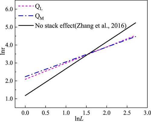
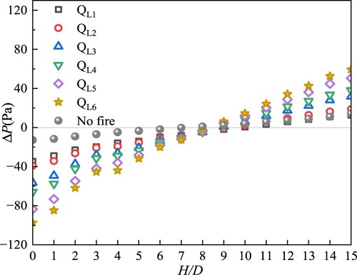
Figure 13. Distribution of differential pressure in the shaft at the fully developed stage for low-floor fire cases.

3.4. Variation of thermal pressure difference inside and outside the shaft

Figure 13 shows the pressure difference distribution in the shaft in the fully development stage in the low-floor fire case. We can obtain the height of the neutral plane (i.e. the height of zero pressure difference) in the shaft under different fire powers. Below the neutral plane, the pressure difference between the inside and the outside of the shaft is negative, indicating that the air flow moves from outside the shaft to inside, coinciding with a positive chimney effect, and the further away from the neutral plane, the greater is the pressure difference. It can be seen from the figure that, under the power of each fire source, an extreme pressure difference appears on the first floor (H/D = 1), the maximum value reaching 97.6 Pa, and the pressure difference at the 15th floor (H/D = 15) is 59.4 Pa. In winter, the temperature inside the shaft is higher than that outside the shaft. The fire aggravates the temperature difference between inside and outside the shaft, the chimney effect is enhanced, and the internal and external pressure difference increases. The temperature at the top of the shaft is lower than that at the bottom, so the pressure difference is smaller than that at the bottom of the shaft. The larger is the power of the fire source, the higher the temperature difference between the shaft and the outside environment, and the larger the internal and external pressure difference.

Figure 14 shows the distribution of pressure difference in the shaft at the fully developed stage of the fire condition on the middle floor. The pressure difference below the fire floor (H/D = 5) has no obvious difference with the increase of height. The chimney effect caused by the ambient temperature difference in this area is dominant, while the thermal buoyancy effect caused by the fire source increases with increasing height below the fire floor, so the pressure difference of these floors is roughly equal under the effect of the two. However, above the fire floor, the further away from the neutral plane, the greater the pressure difference. At this time, the extreme pressure difference under the power of each fire source appears at the 15th floor (H/D = 15), and the maximum is 38.9 Pa, which is reduced by 10.5 Pa compared with the low-floor fire. Compared with the fire on the low floor, the fire on the middle floor reduces the ascending path of the hot smoke and the gradient pressure difference is smaller. The hot smoke sucked into the shaft is less, and the gas in the shaft has less heat energy, which leads to a decrease of the pressure difference at the top of the shaft.

Figure 14. Distribution of differential pressure in the shaft at the fully developed stage for middle-floor fire cases.

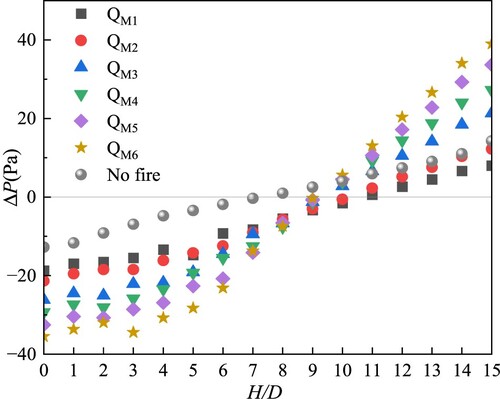
In this article, the neutral surface is initialised at half the height of the shaft, which is the 8th floor of the shaft structure (H/D = 8). The neutral surface of the shaft in the low floor fire is roughly distributed on the 9th floor (H/D = 9), while the neutral surface of the middle floor fire is roughly distributed on the 10th floor (H/D = 10). It can be seen that, within a certain range (below the neutral plane), the higher the position of the fire source, the more obvious is the neutral plane shift.

4. Conclusion

In this article, an elevator shaft model for high-rise buildings is simplified, and the two-dimensional numerical calculation method is adopted to simulate the shaft fire conditions under different fire source positions and different fire powers. The main conclusions are as follows.

1. In the case of a low-floor fire, the higher the power of the fire source, the greater the driving force of the rising smoke, the faster the rising speed, and the shorter the time for smoke to reach the top of the shaft. In a position close to the fire source, the flow structure in the shaft exhibits periodic changes. The further away from the fire source, the more complicated the flow becomes, and periodic changes no longer appear. The smaller the power of the fire source is, the more uniform the distribution of temperature rise in each layer in the shaft. The temperature rise in the shaft structure decreases with the increase of height on the whole, and the average dimensionless temperature rise above 8th floor is basically unchanged.

2. In cases of fire on low and middle floors, the rising smoke dimensionless time is exponentially related to the dimensionless height, but the rising smoke speed of a middle floor fire is slightly faster than that of a low floor fire. Compared with conditions without considering the chimney effect, the flue gas rising speed is relatively slow when Z < 4.609 (below the 4th∼5th floors), and faster when Z > 4.609 (above the 4th∼5th floors).

3. The further away from the neutral surface, the greater the pressure difference between inside and outside the shaft. The extreme fire pressure difference on the low floors appears on the first floor (97.6 Pa), and the extreme fire pressure difference of the middle floor appears on the 15th floor (38.9 Pa). Fire causes the neutral surface of the shaft to shift, and below the original neutral surface, the higher the fire source position, the more obvious the neutral surface shift.

4. Variation of flue gas temperature in an axial structure under the combined effect of hot smoke buoyancy and the chimney effect, obtained in this article, can provide a theoretical basis and practical guidance for practical fire prevention design and the evacuation of people in high-rise buildings. The close location of neutral surfaces helps to adopt corresponding smoke control strategies for fires on different floors.

Limitations, improvements and future direction

Temperature is a more significant factor, directly reflecting the motion of the flue gas in the shaft. In this article, we have only analysed and studied the properties reflected by the temperature in the central axis of the shaft. Further studies could be carried out on other factors such as the CO concentration in the central axis of the shaft and the flue gas particles.

Disclosure statement

No potential conflict of interest was reported by the authors.

Additional information

Funding

This research was funded by the General Program of Natural Science Foundation of Hebei Province of China [grant number E2022210069]; the National Natural Science Foundation of China [grant number 11802186]; the innovation research group project of the Natural Science Foundation of the Hebei Province of China [grant number E2022210078]; the Science and Technology Winter Olympics Special Project [grant number 21475402D]; the High-End Talents Project of the Hebei Province of China [grant number (2019) 63].

References

- Ahn, C. S., Bang, B. H., & Kim, M. W. (2019). Theoretical, numerical, and experimental investigation of smoke dynamics in high-rise buildings. International Journal of Heat and Mass Transfer, 135, 604–613. https://doi.org/10.1016/j.ijheatmasstransfer.2018.12.093
- ASHRAE. (2009). ASHRAE Handbook-Fundamentals. Atlanta: American society of heating. Refrigerating and Air-Conditioning Engineers, 9–13.
- Cheng, L., Zhu, Y. F., & Band, S. S. (2021). Role of gradients and vortexes on suitable location of discrete heat sources on a sinusoidal-wall microchannel. Engineering Applications of Computational Fluid Mechanics, 15(1), 1176–1190. https://doi.org/10.1080/19942060.2021.1953608
- Cui, H., Wang, W. Y., Xu, F., Suvash, C. S., & Liu, Q. K. (2022). Transitional free convection flow and heat transfer within attics in cold climate. Thermal Science, 26(6A), 4699–4709. https://doi.org/10.2298/TSCI210826039C
- He, J. J., Huang, X. Y., & Ning, X. Y. (2020). Stairwell smoke transport in a full-scale high-rise building: Influence of opening location. Fire Safety Journal, 117, 103151. https://doi.org/10.1016/j.firesaf.2020.103151
- He, J. J., Huang, X. Y., & Ning, X. Y. (2022). Modelling fire smoke dynamics in a stairwell of high-rise building: Effect of ambient pressure. Case Studies in Thermal Engineering, 32, 101907. https://doi.org/10.1016/j.csite.2022.101907
- Ji, J., Li, L. J., & Shi, W. X. (2013). Experimental investigation on the rising characteristics of the fire-induced buoyant plume in stairwells. International Journal of Heat and Mass Transfer, 64, 193–201. https://doi.org/10.1016/j.ijheatmasstransfer.2013.04.030
- Klote, J. H. (1993). Zone fire modeling with natural building flows and a zero order shaft model. National Institute of Standards and Technology.
- Li, L. (2014). Study on smoke transport law in vertical channel of high-rise building and fire behavior characteristics of fire room [Master's thesis, University of Science and Technology of China]. University of Science and Technology of China Theses and Dissertations Archive. https://kns.cnki.net/kcms2/article/abstract?v=o5pxseSVRjwsM7hmLfz3stkP_0UVIVRhstkoqD2jPIkuzxTtJYCZSFqV8Q2IVZSg9XygazaGIsurS_2JoUGzLo3ci8OsBDY6FhqhxLlQvVcVaAmgTcYH3A===uniplatform=NZKPT&language=CHS.
- Li, L. J., Ji, J., & Fan, C. G. (2014). Experimental investigation on the characteristics of buoyant plume movement in a stairwell with multiple openings. Energy & Buildings, 68(pt.A), 108–120. https://doi.org/10.1016/j.enbuild.2013.09.028
- Li, M. (2018). Research on fire development mechanism and smoke control under multi-factors of high-rise buildings [Master's thesis, University of Science and Technology of China.] University of Science and Technology of China Theses and Dissertations Archive. https://kns.cnki.net/kcms2/article/abstract?v=o5pxseSVRjxFY3h3e2KdSoQrMVYwVsuiBIcP7zAJlNzxkm3stx2oNToxLbxn5atR3xw2v5oYN5ASD_SC5QZmXRbgmAEhHY4IE7Whff_xI7b62CtFB9W9_DK9OD05ZlA9&uniplatform=NZKPT&language=CHS.
- Lu, Y., Li, G., & Liu, J. (2018). Field measurement and analysis of chimney effect of super high-rise residential buildings in severe cold area. Building Science, 34((08|8)), 1–9 + 31. https://doi.org/10.13614/j.cnki.11-1962/tu.2018.08.01
- Mao, S. H. (2012). Theoretical model and experimental study of smoke neutral surface [Doctoral dissertation, University of Science and Technology of China]. University of Science and Technology of China Theses and Dissertations Archive. https://kns.cnki.net/kcms2/article/abstract?v=o5pxseSVRjwej_Dt6EonrHZqHP_mmB8zX_nkF0ykuk_yfcVZef65k7WGdbavnFfEezI946Go2imFbm5wiKKdMXXyR3NVStZDebOMiVJT13e5toYuAkB5HQ===uniplatform=NZKPT&language=CHS.
- Sergio, G., Marcelo, R., & Francois, F. (2011). Assessment study of K-ε turbulence models and near-wall modeling for steady state swirling flow analysis in draft tube using fluent. Engineering Applications of Computational Fluid Mechanics, 5(4), 459–478. https://doi.org/10.1080/19942060.2011.11015386
- Shi, W. X., Ji, J., & Jin, H. (2014). Experimental study on influence of stack effect on fire in the compartment adjacent to stairwell of high rise building. Journal of Civil Engineering and Management, 20(01), 121–131. https://doi.org/10.3846/13923730.2013.802729
- Sun, X. Q., Hu, L. H., & Li, Y. Z. (2009). Studies on smoke movement in stairwell induced by an adjacent compartment fire. Applied Thermal Engineering, 29(13), 2757–2765. https://doi.org/10.1016/j.applthermaleng.2009.01.009
- Tanaka, T., Fuijia, T., & Yamaguchi, J. (2000). Investigation into rise time of buoyant fire plume fronts. International Journal on Engineering Performance-Based Fire Codes, 2(1), 14–25.
- Wu, J. (2018). Chimney effect of super high-rise building and its HVAC system design [Master's thesis, Beijing University of Architecture]. Beijing University of Architecture eTheses Repository. https://kns.cnki.net/kcms2/article/abstract?v=o5pxseSVRjy1WPGHdtykDxd9e6_aG7mqUmWUEzHbl5C7_NMfL1glmvECLb2WA2ZHqBluuY9BE1m2LOFzjsDQi0ymgxDwrzO5fNmXG6gqwCDX4GCwLn76zQ===uniplatform=NZKPT&language=CHS.
- Xie, T. G., & Huang, X. (2019). Chimney effect fire protection design of elevator shaft in high-rise building. Fire Science and Technology, 38(03|3), 352–355. https://doi.org/10.3969/j.issn.1009-0029.2019.03.013
- Xie, Y., Liu, X., & Zhang, C. Q. (2021). Coupled heat transfer model for the combustion and steam characteristics of coal-fired boilers. Engineering Applications of Computational Fluid Mechanics, 15(1), 490–502. https://doi.org/10.1080/19942060.2021.1890227
- Xu, X. Y., Li, Y. Z., & Mao, S. H. (2011). Continuum model for predicting the position of the neutral surface of shafts in case of fire. Combustion Science and Technology, 17(04|4), 375–381.
- Yin, H. B. (2015). Analysis of combined effect of chimney effect simulation and wind pressure of super high-rise building [Master's thesis, South China University of Technology] South China University of Technology eTheses Repository. https://kns.cnki.net/kcms2/article/abstract?v=o5pxseSVRjzEQTY8vCK1Rqg_eCA4L97Nlt0X7B9qq2pyTG0zWoKnhQnytyiDB0Hlfv_Sjxh9F9XiYWOfx6NwcBoah503SaX5mwWJ2b9MMS51WxNc2TiZUg===uniplatform=NZKPT&language=CHS.
- Zhang, J. Y. (2016). Study on smoke flow characteristics and control in high-rise building shaft [Master's thesis, University of Science and Technology of China] University of Science and Technology of China Theses and Dissertations Archive. https://kns.cnki.net/kcms2/article/abstract?v=o5pxseSVRjw_b5oFLpwidX0ONYqGShwKbIRoYe6vBARToKZ5TMAfp3N2qBMAbi8ObTmUFoIZn_lz5SQsB96MEev79kDsuR1RgIGXIhdcQ6afxuFNXAlqMQ===uniplatform=NZKPT&language=CHS.
- Zhang, J. Y., Li, Y. Z., & Huo, R. (2006). Experimental study on the rising time of plume front in a shaft [J]. Journal of Safety and Environment, (02|2), 111–114.
- Zhang, S. (2011). Computational fluid dynamics and Its applications: Principles and applications of CFD software. Huazhong University of Science and Technology Press.
- Zhu, L. Q., Yuan, X. Y., & Gao, Z. H. (2020). Experimental investigation of effect of external side wind on fire behaviors in a corridor connected to a shaft. Fire Technology, 56(2), 863–881. https://doi.org/10.1007/s10694-019-00907-8