Approximating heat loss in smart buildings through large scale experimental and computational intelligence solutions

Abstract

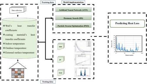
The attainment of energy sustainability in the building sector can be realised by implementing a green building programme, which has grown significantly over the last thirty years. Green building is considered a technical and management strategy within the building and construction industries. Many different prediction methods, both complex and simple, have been put out in recent years and used to solve a wide variety of issues. Several case studies have highlighted factors that impede energy and resource usage in green buildings. The utilisation, trends, and consequences of wall and thermal insulation materials are examined. The main scope of this investigation is to predict buildings’ heat loss by applying artificial neural networks according to the heat transfer coefficients of walls and coating materials, as well as indoor, outdoor, and external surface temperatures. The data has been normalised and presented to two selected neural networks (Harmony search (HS) and particle swarm optimisation are used and contrasted (PSO)). For evaluating the accuracy of models, two statistical indexes are used (R² and RMSE). Model performance of PSO-MLP is shown by R² amounts of 0.97055 and 0.87381, respectively, and RMSE amounts of 0.02534 and 0.09685. Similarly, HS-MLP model accuracy is also indicated by R² amounts of 0.93839 and 0.84176 and RMSE amounts of 0.03635 and 0.10753. The analysis in this paper shows that PSO-MLP predicts heat loss with higher accuracy and improved performance.

KEYWORDS:

• Green buildings
• heat loss
• harmony search
• particle swarm optimisation
• artificial neural network

1. Introduction

Buildings in Europe are responsible for 36% of all CO2 emissions and 40% of all energy usage (Bemani et al., 2020; Recast, 2010). Predicting the energy usage amount is essential in buildings to optimise energy performance and reach energy protection (Chen et al., 2022; Faroughi et al., 2020). However, due to the wide variations in energy kinds and building types, the energy system in structures is highly complicated (Tao et al., 2023). Cooling load, heating load, hot water, and electricity are the primary energy sources considered in the literature. The three building kinds most usually considered range from little apartments to vast estates: office, residential, and technical structures (Moayedi, Yildizhan, Aungkulanon, et al., 2023). The weather, particularly the temperature, construction of buildings and the physical components’ thermal features used, the occupation and how they behave, all have an impact on a building’s energy behaviour (Khosravi et al., 2023).

The intricacy of the issue makes accurate consumption forecasts challenging (Yang et al., 2023). Many different prediction methods, both complex and simple, have been put out in recent years and used to solve a wide variety of issues. This investigation work has been done in the design, operation, or retrofit of modern structures, ranging from local, state, or federal modelling to examining the building’s subsystems. Predictions may be made for the whole structure or individual sub-level elements by carefully examining each affecting aspect or by estimating the use by considering several important variables (Faroughi et al., 2020).

As early as the early 1990s, investigators created various modelling techniques to forecast building energy requirements (Adnan, Dai, Kuriqi, et al., 2023; Adnan, Mostafa, et al., 2023). Engineering, AI-based, and hybrid methods may be used to categorise these technologies further (Foucquier et al., 2013). The engineering technique, a building component’s energy utilisation or the complete building, determines energy usage by utilising thermodynamic equations to model the systems’ physical treatment and their relevance with the environment (Zhao & Magoulès, 2012). The fundamental logic of this strategy is known as the ‘white box,’ thus the name (Moayedi & Khasmakhi, 2023). The AI-based strategy, which differs from the engineering approach, is known as the ‘black box’ since it forecasts energy usage without understanding the fundamental relationships between the building and its constituent parts. The ‘grey box’ hybrid technique compounds the black-box and white-box approaches to get around each approach’s drawbacks. Grey-box and white-box techniques are time-wasting and need laborious expert effort for method creation. They both require precise architectural data to simulate the underlying relations to forecast energy usage (Shi, 2023). Using these two techniques for available structures’ analysis and their energy consumption becomes laborious because, if not impossible, it may be challenging to precisely gather information on the mechanical and building envelope specifications, preventing their widespread application to the existing building stock (Lin et al., 2011). The modern AI-based approaches are covered in-depth in this work for forecasting energy in buildings, while a full evaluation of tools for predicting energy usage is accessible (Foucquier et al., 2013). A single prediction technique using a single learning algorithm and an ensemble prediction approach combining several single prediction techniques to increase prediction accuracy is investigated and contrasted (Ikram, Hazarika, et al., 2023).

Building energy usage is predicted using an AI-based algorithm based on associated variables, including environmental factors, building attributes, and occupancy levels (Xu et al., 2020). AI-based algorithms have been utilised in predicting building energy usage due to their effectiveness in making predictions (Zhang et al., 2021). The AI-based approaches and other forecast techniques for building energy usage have been compared in earlier research. To illustrate: Turhan et al. (2014) contrasted the Back Propagation Neural Network (BPNN) with KEP-IYTEESS to indicate the green buildings’ heating load; Neto and Fiorelli (2008) contrasted EnergyPlus with Artificial Neural Network (ANN), for anticipating energy usage in the building; and more. This research showed that AI-based systems are the most effective for predicting the energy usage of existing building stock since they have benefits over-engineering and hybrid techniques like model simplicity, computation speed, and learning capacity (Kannan & Neeharika, 2007). AI model creation is quick because of its simple architecture and experimental data-collecting requirements (Adnan Ikram et al., 2023; Ikram, Dehrashid, et al., 2023; Yang et al., 2022). For example, the consecutive processes of the software structure cause energy simulation engines like EnergyPlus, which can model complex structures, to operate relatively more slowly than AI-based methods. For example, the space temperature is upgraded hourly, utilising feedback from the HVAC module. Furthermore, using time series data, AI-based methods may forecast future energy usage behaviour (Xiao et al., 2022). In contrast, energy modelling software uses a more traditional forward approach and provides energy prediction for known structures on a yearly, monthly, hourly, or 15-minute basis (Ikram, Dehrashid, et al., 2023). In contrast to simulation methods of energy in buildings, AI-based models have the significant advantage of requiring a small variables’ number that accurately describe the function of the building as a system (J. Wang, Tian, et al., 2022).

The information is set up in the following manner. Section 2 evaluates current research by categorising it following the model in use. The discussion and areas for further study are included in Section 3, and our findings are covered in Section 4.

2. Experimental plan

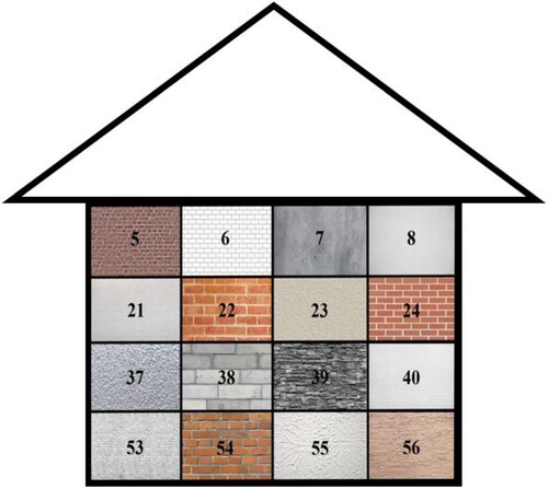
Because of rising energy costs and climate changes, it was necessary to decrease the consumption of energy resources based on carbon (Nabipour et al., 2020). Among the most successful strategies in this respect is installing thermal insulation on structures. Using less energy for building heating, cooling, and insulating heat, CO2 emissions are reduced. This study used experimental research to evaluate the impact of different thermal insulation materials on the emission of CO₂ in the climate of Hakkari. The function of energy in various kinds of walls (aerated concrete, red brick, briquette, and reinforced concrete), along with their impacts on CO2 emissions, were evaluated using various insulating compounds (plaster, aerogel, xps, and eps) for this goal (Figure 1).

Figure 1. A view of different walls.

2.1. Established database

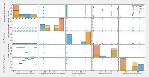
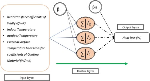
The research’s outcome parameter is heat loss. The research’s input variables include the wall’s and coating material’s heat transfer coefficient, the room, outside, and the external surface temperature. The distribution input and output layers are illustrated in Figure 2. Figure 3 demonstrates four graphs that show the variation of input parameters two by two, and Figure 4 indicates the variation of input parameters. The output parameter (Heat loss) is categorised into three classes I, II, and III. According to this classification, class I ranges between 0.3762 and 12.5, class II ranges between 12.6 and 25, and class III ranges between 25.1 and 36.5654.

Figure 2. The graphical view of the output and input variables.

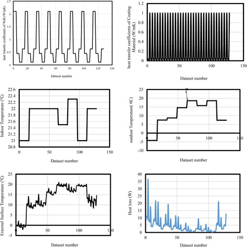
Figure 3. Variation of the input layers. (a) Wall’s heat transfer coefficients-coating material’s heat transfer coefficients; (b) Indoor temperature-Outdoor temperature; (c) Wall’s heat transfer coefficients-External surface temperature; (d) Coating material’s heat transfer coefficients-External surface temperature.

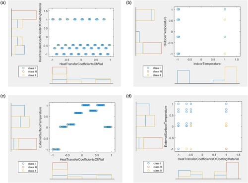
Figure 4. Variation of the input layers.

3. Methodology

This study employs two methods, namely harmony search (HS) and particle swarm optimisation (PSO) in conjunction with artificial neural networks (ANN) to estimate heat loss in green buildings. As previously mentioned, the aim of this study is to determine the extent of heat loss in such structures. In light of the fact that HS, PSO, and ANN have been extensively discussed in previous literature, the present study includes supplementary descriptions of these concepts. This study aimed to create a novel hybrid technique, specifically HS-ANN and PSO-ANN. Consequently, this section provides an overview of PSO and HS for contextualisation purposes. Figure 5 provides an elaborate depiction of the study’s particulars.

Figure 5. Current study’s flowchart.

3.1. Artificial neural network

The most popular artificial intelligence models for predicting building energy usage are ANNs (Qasem et al., 2019). This model is a successful strategy for this challenging application since it is proficient at tackling non-linear issues (Adnan, Dai, Mostafa, et al., 2023). Researchers used ANNs to analyse different kinds of building energy usage in various situations over the past 20 years, including cooling, heating, electricity usage, sub-level components’ optimisation and operation, and determination of consumption variables (Gu et al., 2023; Moayedi, Yildizhan, Al-Bahrani, et al., 2023; Zheng & Yin, 2022). We discuss the prior research in this part. Figure 6 depicts a schematic depiction of an ANN structure.

Figure 6. An MLP structure for the current article.

The ANNs’ use in buildings’ energy problems was briefly reviewed by Kalogirou (Kalogirou, 2006) in 2006. Backpropagation neural networks were utilised by Kalogirou et al. (1997) to forecast the necessary heating demand for buildings. The data from 225 buildings, ranging from tiny areas to huge rooms, were used to train the model. A similar technique was used by Ekici and Aksoy (2009) to forecast the heating loads of buildings in three structures. The yearly heating requirements of many modest single-family houses in northern Sweden were projected by Olofsson et al. (1998). Later, Olofsson and Andersson (2001) created a neural network with a high forecasting rate for single-family houses that predicts long-term energy consumption (the yearly heating requirement) based on short-term (usually 2–5-week) observed data.

To forecast cooling demand in a structure, Yokoyama et al. employed a BPNN (Yokoyama et al., 2009). In their study, the identification of model parameters was suggested using a global optimisation technique termed the modal trimming approach. Using hourly energy use data and a recurrent neural network, Kreider et al. (1995) could forecast future building heating and cooling requirements using just the current time stamp and weather. Ben-Nakhi and Mahmoud (2004) projected the cooling demand of three office buildings utilising the same recurrent neural network. For model training, a database of the cooling load was utilised (from 1997 to 2000), and for testing the method, a database from 2001 was utilised. To anticipate a passive solar building’s energy usage without the need for mechanical or electrical heating systems, Kalogirou (Kalogirou & Bojic, 2000) employed neural networks. Cheng-wen and Jian (2010) employed a BPNN to estimate the cooling and heating load of buildings in distinct climatic areas defined by cooling and heating degree per day, considering the impact of weather on energy usage in various locations. These two energy measurements served as training inputs for the neural network.

A lot of the time, for HVAC systems, ANNs are also utilised to study and improve the behaviour of sub-level components (Kargar et al., 2020; Shabani et al., 2023). The prediction of air-conditioning load in a building by Hou et al. (2006) is crucial for the HVAC system’s best management. A broad regression neural network was utilised by Lee et al. (2004) to identify and diagnose issues with air-handling equipment in a building. According to Aydinalp et al. (2002), the neural network may be utilised to predict the energy usage of appliances, lights, and space cooling in the Canadian residential sector. It is also a useful model for estimating the influence of socioeconomic variables on this usage. In their further research, neural network models were created to accurately predict household hot-water heating and space heating energy usage in the same industry (Aydinalp et al., 2004).

The number of hidden layers and the number of neurons in each layer are two critical design parameters that can significantly impact the performance of an ANN (Moayedi, Canatalay, Ahmadi Dehrashid, et al., 2023). Here’s how they each play a significant role (Zhang et al., 2023):

The number of Hidden Layers: The number of hidden layers determines the complexity of the ANN’s architecture. A shallow neural network with one or two hidden layers may be sufficient for simple problems, but for more complex problems, a deep neural network with multiple hidden layers may be required. Deep neural networks can learn hierarchical representations of data, which can help them capture more complex relationships between input features and output variables (Du et al., 2023).

However, increasing the number of hidden layers can also make the network more difficult to train, as vanishing or exploding gradients can occur during backpropagation. To mitigate this problem, various techniques, such as batch normalisation, residual connections, and skip connections, have been developed to improve the training of deep neural networks.

Number of Neurons: The number of neurons in each layer determines the capacity of the network to learn complex patterns. Many neurons can help the network model complex nonlinear relationships between input features and output variables. Still, it can also lead to overfitting if the network is improperly regularised.

On the other hand, a small number of neurons can limit the network’s capacity to learn complex patterns, leading to underfitting. Therefore, the number of neurons should be chosen carefully based on the problem’s complexity and the dataset’s size. Table 1 shows the outcomes of the neural network.

Table 1. The optimisation outcomes of neural network.

	Network outcomes			Scoring
Neurons’ number	RMSEtotal	RMSEtrain	RMSEtest	RMSEtotal	RMSEtrain	RMSEtest	Total score	Rank
1	0.117	0.201	0.147	10	10	10	30	1
2	0.555	0.544	0.552	2	2	2	6	9
3	0.440	0.392	0.426	5	6	5	16	6
4	0.534	0.421	0.504	3	4	3	10	8
5	0.167	0.304	0.217	9	8	9	26	2
6	0.362	0.356	0.360	7	7	7	21	4
7	0.416	0.409	0.414	6	5	6	17	5
8	0.247	0.280	0.258	8	9	8	25	3
9	0.612	0.624	0.615	1	1	1	3	10
10	0.447	0.452	0.448	4	3	4	11	7

3.2. Hybrid model development

Three performance metrics, namely, root-mean-squared error (RMSE), determination coefficient (R²), and mean absolute error (MAE), were employed to evaluate the quality of the HS-MLP and PSO-MLP samples (R²). Equations (1)–(3) explained the RMSE, R², and MAE computation. (1) $\begin{array}{rl}\text{RMSE}& =\sqrt{\frac{1}{n}\sum _{i=1}^n{\left(y_i-{\hat{y}}_i\right)}^2}\end{array}$(1) (2) $\begin{array}{rl}{R}^2& =1-\frac{{\sum }_i{\left(y_i-{\hat{y}}_i\right)}^2}{{\sum }_i{\left(y_i-\overline{y}\right)}^2}\end{array}$(2) (3) $\begin{array}{rl}\text{MAE}& =\frac{1}{n}\sum _{i=1}^n|y_i-{\hat{y}}_i|\end{array}$(3) where n denotes the occurrences’ number and $\overline{y}$, $y_i$, and ${\hat{y}}_i$ are taken to represent the response variable’s average, estimated, and modelled quantities, respectively.

3.3. Harmony search (HS)

Each solution in the fundamental HS method is referred to as a ‘harmony’ and is defined as an n-dimensional real vector (Geem et al., 2001). Harmony memory stores a randomly generated starting harmony vector population (HM). Then, utilising a rule of considering memory, modifying pitch, and accidental re-initialisation, a recent volunteer harmony is created from each of the explanations in the HM (Lee & Geem, 2004). The HM is finally upgraded by contrasting the new volunteer harmony with the HM’s worst harmony vector. If the new volunteer vector is superior to the weakest vector of harmony in the HM, it will take its place. Until a specific termination criterion is satisfied, the procedure above is repeated. Here’s a flowchart of the Harmony Search algorithm (Haghshenas et al., 2021):

1. Initialise the harmony memory with random solutions.

2. Evaluate the objective function for each solution.

3. Determine the best solution in the harmony memory.

4. Generate a new solution by combining existing solutions in the memory (harmony improvisation).

   • - Choose a random index i and a random value from the i-th column of the harmony memory.

   • - Generate a new value for the i-th column based on a random probability.

   • - If the new value is better than the current value, replace the current value with the new value.

5. Evaluate the objective function for the new solution.

6. Update the harmony memory by replacing the worst solution with the new solution if it is better.

7. Repeat steps 3–6 until a stopping criterion is met (e.g. the maximum number of iterations or convergence).

8. Return the best solution found in the harmony memory.

3.3.1. Issue initialisation and variable of algorithm

The overall solution to the global optimisation issue is as bellows: The objective function is min f(x) st: x(j) $\in$ [LB(j), UB(j)], j = 1,2, … , n, the set of design parameters is x = (x(1), x(2), … , x(n)), and the number of design parameters is n, and the upper limit and lower limit for the design parameter x(j) are LB(j) and UB(j), respectively (Shaffiee Haghshenas et al., 2022).

The harmony memory size, also known as the several vectors of solution in harmony memory (HMS), rate of pitch adjusting (PAR), distance bandwidth (BW), consideration rate of harmony memory (HMCR), as well as several improvisations, are the HS algorithm (NI) parameters. All function evaluations and the NI are the same. Selecting the right parameters will improve the network’s capacity to find the global optimum or an area close to it with a high convergence rate.

3.3.2. Initialise the harmony memory (HM)

HMS harmony vectors make up the HM. Let $X_i$ = {$x_i$ (1), $x_i$ (2), … , $x_i$ (n)} denote the ith harmony vector, which is created at random according to $x_i\left(j\right)$ = LB(j) + (UB(j) _ LB(j)) × r, where r exists as a uniform accidental number among 0 and 1, i = 1,2, … , HMS and j = 1,2, … , n. The HMS harmony vectors are then added to the HM matrix in the manner described below: (4) $\begin{array}{r}\text{HM}=\left[\begin{array}{c}{X}_1\\ X_2\\ \begin{array}{c}\dots \\ X_{\text{HMS}}\end{array}\end{array}\right]\end{array}$(4)

3.3.3. Devise a new harmony

Three criteria are used to devise a new harmony vector, $X_{\text{new}}$: considering memory, a pitch adjustment, along with a haphazard choice. An accidental number is first produced in the [0, 1] range. The memory consideration generates the decision variable $x_{\text{new}}\left(j\right)$ if $r_1$ is smaller than HMCR; else, a random selection is used to produce $x_{\text{new}}\left(j\right)$ (that is, accidental re-initialisation among the search bounds). $x_{\text{new}}\left(j\right)$ is chosen from any i vector of harmony in {1, 2, … , HMS} for the memory concern. Second, if a decision variable is upgraded by considering the memory, it will be pitched adjusted with a possibility of PAR. Following is the pitch adjustment rule: (5) $\begin{array}{r}{x}_{\text{new}}\left(j\right)=x_{\text{new}}\left(j\right)\pm r\times \text{BW}\end{array}$(5) where r is an integer generated uniformly randomly between [0, 1].

3.3.4. Update harmony memory

The harmonic memory is upgraded through the fittest competition’s survivorship among the most recent vector of harmony, $X_{\text{new}}$, and the previous vector of harmony, $X_{\text{W}}$, in the HM. If $X_{\text{new}}$’s fitness value is higher than $X_{\text{W}}$’s, $X_{\text{new}}$ will take the position of $X_{\text{W}}$ and join the HM.

3.4. Particle swarm optimization (PSO)

PSO is an algorithm that draws inspiration from the behaviour of particles and social creatures like birds and fish. PSO is an accidental optimisation approach that Eberhart and Kennedy devised and refined (Eberhart & Kennedy, 1995). It was even categorised as a heuristic method. The initial aim of the PSO method is to modify social information trade between people in a group. Each one treats as a particle inside the population. Then they do a search process in a search area (B. Wang, Rahbari, et al., 2022). They exchange wisdom and expertise to update better places while searching (Nguyen et al., 2020). As a result, it was also regarded in the statistical field as an evolutionary computing approach (Armaghani et al., 2014; Gordan et al., 2016; Moayedi et al., 2019; Moayedi et al., 2020; Nguyen et al., 2020; Yang et al., 2019). The PSO algorithm uses five phases to provide the best possible search (Mikaeil et al., 2018):

• - Step 1: Establish the particle velocity and native population in step 1. The next step is calculating the particle’s fitness and identifying the local and global optimum locations.

• - Step 2: With the starting velocity determined in Step 1, each particle travels radially in the search space. The speed is determined by both regional and international best. The best outcome corresponds to the local greatest per loop, and the greatest particle’s position so far corresponds to the global greatest. Alternatively, the velocity is modified in this phase to match the local best and global greatest per loop (Guido et al., 2022). As said, it is: $\begin{array}{rl}{v}_j^{i+1}& =w{v}_j^{\left(i\right)}+\left(c_1\times r_1\times \left(\text{local bes}{\text{t}}_j-x_j^{\left(i\right)}\right)\right)\\ & +\left(c_2\times r_2\times \left(\text{global bes}{\text{t}}_j-x_j^{\left(i\right)}\right)\right),\\ & \times v_{\text{min}}\le v_j^{\left(i\right)}\le v_{\text{max}}\end{array}$

where $r_1$ and $r_2$ represent integers in the [0,1] interval, $x_j^{\left(i\right)}$ signifies the location of the particles, $v_j^{\left(i\right)}$ represents the jth particle’s speed at the ith repetition, w denotes the inertial weight’s coefficient, and i is the repetitions’ number (Guido et al., 2020).

• - Step 3: The particles move at the upgraded velocity within the search space once the new velocity has been estimated and upgraded. Each position’s fitness is assessed and adjusted accordingly using a fitness function.

• - Step 4: Update global and local greatest for the best situation with the lowest RMSE in step 4. The most recent local situation might be: (6) $\begin{array}{r}{x}_j^{i+1}=x_j^{\left(i\right)}+v_j^{\left(i+1\right)};j=1,2,\dots ,n\end{array}$(6)

• - Step 5: Verify that your search was successful. Stop the search if the particle has the highest fitness (lowest RMSE). If not, go to step 2 again.

4. Results and discussion

In the current step, 80% of the total database was accidentally chosen to create models for predicting heat loss from buildings, while the remaining 20% was utilised to test the models’ performance. It should be noted that all models employed identical testing and training database and resampling approaches. To accurately predict heat loss from green buildings, it is important to consider the viability of the suggested HS-MLP and PSO-MLP models. The HS and PSO algorithms were integrated with the ANN model. Before completing the ANN model optimisation, the HS and PSO method parameters were ideally determined. The procedure of looking for and optimising for the ANN’s variables was carried out once the HS and PSO algorithm’s parameters had been specified. Figure 7 shows their performance.

Figure 7. The MSE variation for the (a) HSMLP, and (b) PSOMLP suggested methods. (a) HSMLP; (b) PSOMLP.

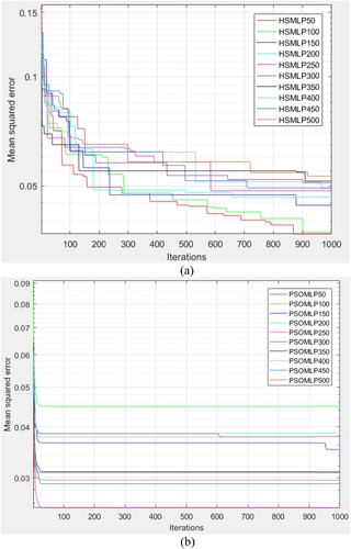
According to Figure 7, an ideal HS-MLP model with a 100-swarm size and the lowest RMSE (RMSE = 0.03635 and 0.10753) and an ideal PSO-MLP model with a 250-swarm size and the lowest RMSE (RMSE = 0.0.02534 and 0.0.09685) were both discovered. The previously mentioned HS-MLP has also been developed for contrast and the developed PSO-MLP model’s general function evaluation.

Two sophisticated computer techniques are devised to forecast the heat loss of residential structures. The method is initially trained to utilise the training dataset. According to the influential variables in buildings’ training and testing datasets, Figures 8 and 9 illustrate how well the proposed model predicts heat loss.

Figure 8. The outcomes of testing and training and dataset for various structures of suggested HSMLP. (a) HSMLP- N_p50;(b) HSMLP- N_p100; (c) HSMLP- N_p150; (d) HSMLP- N_p 200; (e) HSMLP- N_p250; (f) HSMLP- N_p300; (g) HSMLP- N_p350; (h) HSMLP- N_p400; (i) HSMLP- N_p450; (j) HSMLP- N_p500.

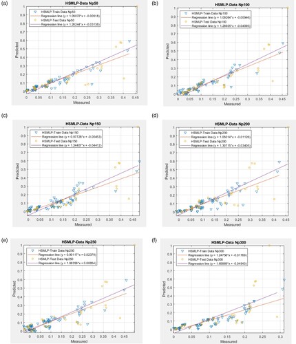
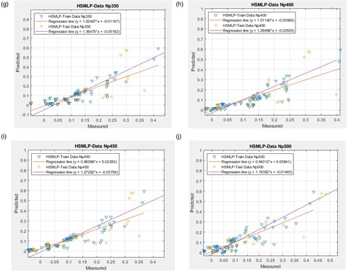
Figure 9. The outcomes of testing and training and dataset for various structures of suggested PSOMLP. (a) PSOMLP- N_p50;(b) PSOMLP- N_p100; (c) PSOMLP- N_p150; (d) PSOMLP- N_p 200; (e) PSOMLP- N_p250; (f) PSOMLP- N_p300; (g) PSOMLP- N_p350; (h) PSOMLP- N_p400; (i) PSOMLP- N_p450; (j) PSOMLP- N_p500.

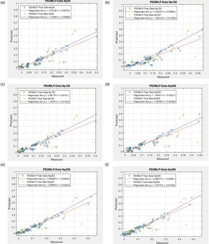
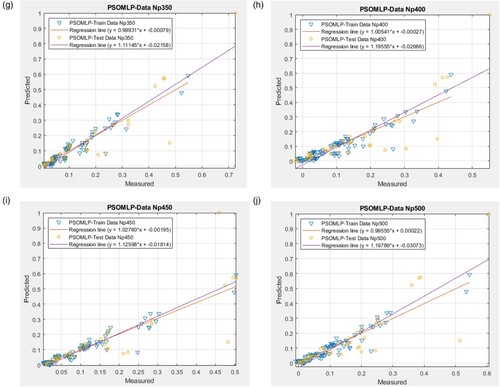
The calculated R² values, however, show that over 70% of goal and output heat losses are consistent. Additionally, for sample sizes of 100 and 250, the estimated training R²s (0.93839 and 0.97055 for HS-MLP and PSO-MLP, respectively) and testing R²s (0.84176 and 0.87381 for HS-MLP and PSO-MLP, respectively), demonstrate the excellent accuracy of the models in forecasting the HL.

Following the creation of the heat loss predicting models, the model’s performance was assessed using observations from the testing dataset using the R² and RMSE, as presented in Tables 2 and 3. The Total Score Ranking (TSR) method was also used to assess the models.

Table 2. The outcomes of network for suggested HSMLP method.

	Training data		Testing data		Scoring
Population size	RMSE	R^2	RMSE	R^2	Training		Testing		Total score	Rank
50	0.03659	0.93755	0.11215	0.8264	9	9	8	8	34	2
100	0.03635	0.93839	0.10753	0.84176	10	10	9	9	38	1
150	0.04366	0.90977	0.11235	0.82572	8	8	7	7	30	3
200	0.04594	0.89956	0.12251	0.78847	5	5	5	5	20	7
250	0.04484	0.90458	0.12277	0.78742	6	7	4	4	21	6
300	0.04705	0.89435	0.14203	0.70108	4	4	1	1	10	8
350	0.05073	0.87598	0.12802	0.76608	2	2	3	3	10	8
400	0.04773	0.89111	0.1357	0.73199	3	3	2	2	10	8
450	0.04484	0.90457	0.11628	0.81189	6	6	6	6	24	4
500	0.05285	0.86459	0.09609	0.87593	1	1	10	10	22	5

Table 3. The outcomes of network for suggested PSOMLP method.

	Training data		Testing data		Scoring
Population size	RMSE	R^2	RMSE	R^2	Training		Testing		Total score	Rank
50	0.03775	0.93336	0.13286	0.74501	4	4	1	1	10	9
100	0.04434	0.90677	0.10649	0.84506	1	1	5	5	12	8
150	0.03518	0.94239	0.12434	0.78121	5	5	2	2	14	7
200	0.03833	0.93122	0.12019	0.79742	2	2	3	3	10	9
250	0.02534	0.97055	0.09685	0.87381	10	10	9	9	38	1
300	0.03084	0.95604	0.0994	0.86656	7	7	8	8	30	3
350	0.03103	0.95548	0.08389	0.90696	6	6	10	10	32	2
400	0.0378	0.93317	0.1037	0.85377	3	3	7	7	20	6
450	0.02887	0.96158	0.10966	0.83478	9	9	4	4	26	5
500	0.0296	0.95957	0.10603	0.84651	8	8	6	6	28	4

The Total Score Ranking Method is a technique used to rank items, participants, or candidates based on their cumulative scores in various categories or criteria. This method is often used in competitions, evaluations, or decision-making processes where multiple factors contribute to each item or individual’s overall performance or value.

Here’s a step-by-step guide to implementing the Total Score Ranking Method:

Identify the criteria: Determine the factors or categories you will use to evaluate and compare the items or participants.

Assign weights to the criteria (optional): If some criteria are more important than others, you can assign weights to each criterion to give them different levels of importance in the overall ranking. If all criteria are equally important, you can skip this step.

Score each item or participant: For each criterion, assign a score to each item or participant. The score can be a numerical value, a letter grade, or any other meaningful assessment (Li et al., 2023).

Calculate the weighted scores (if applicable): Multiply each score by the corresponding weight for the criterion. Then, sum the weighted scores for each item or participant.

Calculate the total scores: Add the scores (or weighted scores) for each criterion to get the total score for each item or participant.

Rank the items or participants: Sort them in descending order based on their total scores, with the highest total score ranked first, and the lowest total score ranked last.

The Total Score Ranking Method provides a quantitative approach to comparison and decision-making. However, it’s important to note that this method is only as accurate and reliable as the criteria and scoring system. Careful consideration should be given to selecting criteria and assigning scores to ensure a fair and meaningful ranking (Gu et al., 2022).

The findings in Tables 2 and 3 supported the complete prediction of the ANN approaches suggested in this work for the heat loss of domestic structures. Having an RMSE of 0.02534, an R² of 0.97055, and a rank of 38, the suggested PSO-MLP sample was determined to be the most effective ANN approach for forecasting the heat loss of residential structures.

The HS-MLP model findings acknowledged the substantial optimisation capacities of the HS method in this research (RMSE = 0.02625 and 0.10753, R² = 0.93839 and 0.84176, total ranking of 38, Table 2). Table 3 clearly shows that the PSO-MLP model performed somewhat better than the HS-MLP model (overall ranking of 38, RMSE = 0.02534 and 0.09685, and R² = 0.97055 and 0.87381). Nevertheless, the PSO-MLP model has surpassed the HS-MLP model in strength.

The efficacy of the model that has been applied is evaluated in this part by comparing the outputs (that is, the anticipated HLs) to the goal values (that is, the estimated HLs). Figures 10 and 11 show the testing and training stages’ outcomes and the differences among each pair of output and goal heat loss. The obtained error values during the training phase for forecasting the HS-MLP (population size = 500) and PSO-MLP (population size = 250) are [−7.8264e-05, 0.037506] and [−0.00060972, 0.025481], respectively.

Figure 10. The error performance for the best fit HSMLP approach. (a) HS 500-training; (b) HS 500-testing.

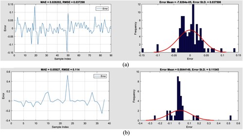
Figure 11. The error performance for the best fit PSOMLP approach. (a) PSOMLP 250-training; (b) PSOMLP 250-testing.

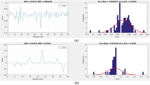
The training RMSE values for the two population sizes of 500 and 250 are 0.037298 and 0.00064246 for HS-MLP and PSO-MLP, respectively. The estimated MAEs (0.026202 and 0.019014) also indicate that both models have little training error.

The RMSEs (0.114 and 0.010324) show how the weights (and biases) modified using HS and PSO algorithms may create useful ANN during the testing phase. Additionally, both algorithms’ MAEs amounts of 0.05927 and 0.053576 exhibit a respectable generalisation error.

4.1. Taylor diagram

In addition to the performance metrics mentioned in the above section, a Taylor diagram has been utilised to investigate its application in the current heat loss issue (Taylor, 2001). The Taylor diagram is a graphical method for comparing the performance of multiple models or simulations against a reference dataset. It was introduced by Taylor (2001) as a way to assess climate models’ skill in reproducing observed variability patterns. The Taylor diagram consists of a polar coordinate system where the reference dataset is located at the origin, and the models or simulations are represented by a set of points on the circle’s circumference. The distance of each point from the origin represents the correlation coefficient (r) between the model output and the reference dataset. In contrast, the angle between the radial line connecting the point to the origin and the horizontal axis represents the difference in the standard deviation (σ) between the model output and the reference dataset. The Taylor diagram provides several advantages over other methods for comparing model performance, such as scatterplots or bar charts. First, it allows for the visualisation of multiple performance metrics (correlation and standard deviation) in a single plot, facilitating the comparison of multiple models or simulations. Second, it allows for evaluating the magnitude and direction of the differences between the model output and the reference dataset, providing a more comprehensive assessment of skill. Finally, it provides a clear and intuitive representation of the trade-offs between correlation and standard deviation, allowing for identifying models that perform better overall or in specific aspects of the variability.

In practice, the Taylor diagram can be used to assess a model’s or simulation’s skill in reproducing observed patterns of variability across multiple variables, regions, or time periods. It can also be used to compare the performance of different models or simulations against a common reference dataset. The Taylor diagram can be particularly useful in fields such as climate science, where evaluating model performance is critical for understanding the causes and consequences of climate change.

The model’s simulations and observations’ agreement in a quantitative view may result from the Taylor diagrams, which illustrate, for each approach, the standard deviation, and the observations’ correlation. Figure 12 demonstrates the Taylor diagram for utilised approaches. In the Taylor diagram’s view closely, it was ascertained that in both train and test stages, the hybrid PSO-MLP results (where an MLP process had been combined with PSO algorithm as an optimiser method) have a better outcome such that a coefficient of determination is 0.97055. Notably, the root mean square error (RMSE) for the hybrid PSO-MLP approach is lower than <0.10. Besides the MLP model with the PSO optimiser approach, the hybrid PSO-MLP approach stands out as the best-predicted model consistent with results.

Figure 12. Taylor diagrams for the best-fit structures of HSMLP and PSOMLP proposed predictive networks. (a) training dataset (b) testing dataset.

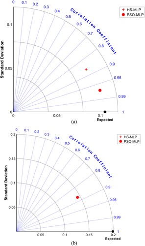
In summary, the Taylor diagram is a powerful tool for comparing and visualising the performance of multiple models or simulations against a reference dataset. Providing a comprehensive assessment of skill across multiple performance metrics can help identify models that perform better overall or in specific aspects of the variability and facilitate the evaluation of model performance in complex and multidimensional problems.

4.2. Model’s restrictions

Both the PSO-MLP and HS-MLP models have certain restrictions and limitations. Here are some of the main ones:

4.2.1. Computational complexity

Both PSO-MLP and HS-MLP models involve the optimisation of multiple hyperparameters, including the number of hidden layers, the number of neurons in each layer, and the learning rate. This optimisation process can be computationally expensive, especially for large datasets or high-dimensional problems.

4.2.3. Overfitting

PSO-MLP and HS-MLP models are prone to overfitting, which occurs when the model is too complex and captures noise or random fluctuations in the training data. Overfitting can lead to poor generalisation performance and reduced new, unseen data accuracy.

4.2.4. Limited interpretability

PSO-MLP and HS-MLP models are black-box models, meaning they do not provide explicit information about the underlying relationships between the input and output variables. This can limit their interpretability and make understanding how the model arrives at its predictions difficult.

4.2.5. Sensitivity to initial conditions

Both PSO-MLP and HS-MLP models are sensitive to the initial conditions and require careful tuning of the algorithm parameters to achieve good performance. This sensitivity can make reproducing the results challenging or applying the models to new datasets or problems.

4.2.6. Limited applicability

PSO-MLP and HS-MLP models are most suitable for problems with continuous input and output variables and may not perform well for problems with categorical or discrete variables. In addition, they may not be suitable for problems with complex or non-linear relationships between the input and output variables.

In summary, while the PSO-MLP and HS-MLP models have shown promising results in some applications, they have certain restrictions and limitations that must be carefully considered when applying them to new problems or datasets. Careful evaluation and validation of the models are necessary to ensure their robustness and reliability.

5. Conclusions

This study proposes two novel estimation methods for residential building heat loss. Five input factors are also considered: the wall and coating material’s heat transfer coefficients and the inside, outside, and external surface temperature. This study demonstrates a way of accurately evaluating the heat loss value of green buildings. Two alternative ANN models are considered and compared in the quest for the best technique (HS-MLP and PSO-MLP). The average accuracy of each one’s heat loss predictions is also used to assess and examine its performance.

One of the key objectives in developing smart cities is to design and optimise the buildings’ heat loss systems. Buildings may become more energy efficient, decrease financial losses, and have a less negative impact on the environment by using HL effectively. Both methods accurately estimate heat loss from residential structures (HS-MLP and PSO-MLP, respectively, RMSE = 0.0.03635 and 0.02534, and R² = 0.93839 and 0.97055). Following are some observations and conclusions based on the study’s findings:

• - HS-MLP and PSO-MLP, two ANN approaches used in this research, were strong candidates for determining heat loss in residential structures. Particularly the suggested PSO-MLP model could estimate a building’s heat loss with great reliability.

• - The PSO-MLP model that was suggested was a reliable method that correctly predicted the building’s heat loss with a favourable outcome (RMSE = 0.02534 and 0.09685, and R² = 0.97055 and 0.87381). As an alternate tool for experimental measures, it should be employed. Building design techniques may also be used based on the suggested PSO-MLP method to reduce heat loss for buildings. Also, the HS-MLP model reached a high accuracy performance.

This investigation shows that ANN approaches can forecast heat loss with a reasonable degree of accuracy regarding historical data commonly recorded. Several mathematical models for calculating heat loss have been suggested in the literature review. It has been observed that previous studies have struggled to strike a balance between accuracy and simplicity when modelling heat loss. However, this article’s results were great for anticipating the residential buildings’ heat loss; further study is required in this issue. For instance, other methods are required to improve their accuracy, or new ANN approaches are developed utilising these methods. Future engineering issues with the scope of energy efficiency containing building design might be done utilising the methods from this study.

Disclosure statement

No potential conflict of interest was reported by the author(s).

References

- Adnan Ikram, R. M., Khan, I., Moayedi, H., Ahmadi Dehrashid, A., Elkhrachy, I., & Nguyen Le, B. (2023). Novel evolutionary-optimized neural network for predicting landslide susceptibility. Environment, Development and Sustainability, 1–33. https://doi.org/10.1007/s10668-023-03356-0
- Adnan, R. M., Dai, H.-L., Kuriqi, A., Kisi, O., & Zounemat-Kermani, M. (2023). Improving drought modeling based on new heuristic machine learning methods. Ain Shams Engineering Journal, 14(10), 102168. https://doi.org/10.1016/j.asej.2023.102168
- Adnan, R. M., Dai, H.-L., Mostafa, R. R., Islam, A. R. M. T., Kisi, O., Elbeltagi, A., & Zounemat-Kermani, M. (2023). Application of novel binary optimized machine learning models for monthly streamflow prediction. Applied Water Science, 13(5), 110. https://doi.org/10.1007/s13201-023-01913-6
- Adnan, R. M., Mostafa, R. R., Dai, H.-L., Heddam, S., Kuriqi, A., & Kisi, O. (2023). Pan evaporation estimation by relevance vector machine tuned with new metaheuristic algorithms using limited climatic data. Engineering Applications of Computational Fluid Mechanics, 17(1), 2192258. https://doi.org/10.1080/19942060.2023.2192258
- Armaghani, D. J., Hajihassani, M., Mohamad, E. T., Marto, A., & Noorani, S. (2014). Blasting-induced flyrock and ground vibration prediction through an expert artificial neural network based on particle swarm optimization. Arabian Journal of Geosciences, 7(12), 5383–5396. https://doi.org/10.1007/s12517-013-1174-0
- Aydinalp, M., Ugursal, V. I., & Fung, A. S. (2002). Modeling of the appliance, lighting, and space-cooling energy consumptions in the residential sector using neural networks. Applied Energy, 71(2), 87–110. https://doi.org/10.1016/S0306-2619(01)00049-6
- Aydinalp, M., Ugursal, V. I., & Fung, A. S. (2004). Modeling of the space and domestic hot-water heating energy-consumption in the residential sector using neural networks. Applied Energy, 79(2), 159–178. https://doi.org/10.1016/j.apenergy.2003.12.006
- Bemani, A., Baghban, A., & Mosavi, A. (2020). Estimating CO2-brine diffusivity using hybrid models of ANFIS and evolutionary algorithms. Engineering Applications of Computational Fluid Mechanics, 14(1), 818–834. https://doi.org/10.1080/19942060.2020.1774422
- Ben-Nakhi, A. E., & Mahmoud, M. A. (2004). Cooling load prediction for buildings using general regression neural networks. Energy Conversion and Management, 45(13-14), 2127–2141. https://doi.org/10.1016/j.enconman.2003.10.009
- Chen, J., Tong, H., Yuan, J., Fang, Y., & Gu, R. (2022). Permeability prediction model modified on Kozeny-Carman for building foundation of clay soil. Buildings, 12(11), 1798. https://doi.org/10.3390/buildings12111798
- Cheng-wen, Y., & Jian, Y. (2010, May 21–24 ). Application of ANN for the prediction of building energy consumption at different climate zones with HDD and CDD. 2010 2nd International Conference on Future Computer and Communication.
- Du, S., Xie, H., Yin, J., Sun, Y., Wang, Q., Liu, H., Qi, W., Cai, C., Bi, G., Xiao, D., Chen, W., Shen, X., Yin, W.-Y., & Zheng, R. (2023). Giant hot electron thermalization via stacking of graphene layers. Carbon, 203, 835–841. https://doi.org/10.1016/j.carbon.2022.12.017
- Eberhart, R., & Kennedy, J. (1995, October 4–6). A new optimizer using particle swarm theory. MHS'95. Proceedings of the sixth international symposium on micro machine and human science.
- Ekici, B. B., & Aksoy, U. T. (2009). Prediction of building energy consumption by using artificial neural networks. Advances in Engineering Software, 40(5), 356–362. https://doi.org/10.1016/j.advengsoft.2008.05.003
- Faroughi, M., Karimimoshaver, M., Aram, F., Solgi, E., Mosavi, A., Nabipour, N., & Chau, K.-W. (2020). Computational modeling of land surface temperature using remote sensing data to investigate the spatial arrangement of buildings and energy consumption relationship. Engineering Applications of Computational Fluid Mechanics, 14(1), 254–270. https://doi.org/10.1080/19942060.2019.1707711
- Foucquier, A., Robert, S., Suard, F., Stéphan, L., & Jay, A. (2013). State of the art in building modelling and energy performances prediction: A review. Renewable and Sustainable Energy Reviews, 23, 272–288. https://doi.org/10.1016/j.rser.2013.03.004
- Geem, Z. W., Kim, J. H., & Loganathan, G. V. (2001). A new heuristic optimization algorithm: Harmony search. SIMULATION, 76(2), 60–68. https://doi.org/10.1177/003754970107600201
- Gordan, B., Jahed Armaghani, D., Hajihassani, M., & Monjezi, M. (2016). Prediction of seismic slope stability through combination of particle swarm optimization and neural network. Engineering with Computers, 32(1), 85–97. https://doi.org/10.1007/s00366-015-0400-7
- Gu, M., Cai, X., Fu, Q., Li, H., Wang, X., & Mao, B. (2022). Numerical analysis of passive piles under surcharge load in extensively deep soft soil. Buildings, 12(11), 1988. https://doi.org/10.3390/buildings12111988
- Gu, Q., Tian, J., Yang, B., Liu, M., Gu, B., Yin, Z., Yin, L., & Zheng, W. (2023). A novel architecture of a six degrees of freedom parallel platform. Electronics, 12(8), 1774. https://doi.org/10.3390/electronics12081774
- Guido, G., Haghshenas, S. S., Haghshenas, S. S., Vitale, A., Astarita, V., & Haghshenas, A. S. (2020). Feasibility of stochastic models for evaluation of potential factors for safety: A case study in southern Italy. Sustainability, 12(18), 7541. https://doi.org/10.3390/su12187541
- Guido, G., Shaffiee Haghshenas, S., Shaffiee Haghshenas, S., Vitale, A., & Astarita, V. (2022). Application of feature selection approaches for prioritizing and evaluating the potential factors for safety management in transportation systems. Computers, 11(10), 145. https://doi.org/10.3390/computers11100145
- Haghshenas, S. S., Haghshenas, S. S., Geem, Z. W., Kim, T.-H., Mikaeil, R., Pugliese, L., & Troncone, A. (2021). Application of harmony search algorithm to slope stability analysis. Land, 10(11), 1250. https://doi.org/10.3390/land10111250
- Hou, Z., Lian, Z., Yao, Y., & Yuan, X. (2006). Cooling-load prediction by the combination of rough set theory and an artificial neural-network based on data-fusion technique. Applied Energy, 83(9), 1033–1046. https://doi.org/10.1016/j.apenergy.2005.08.006
- Ikram, R. M. A., Dehrashid, A. A., Zhang, B., Chen, Z., Le, B. N., & Moayedi, H. (2023). A novel swarm intelligence: Cuckoo optimization algorithm (COA) and SailFish optimizer (SFO) in landslide susceptibility assessment. Stochastic Environmental Research and Risk Assessment, 37(5), 1717–1743. https://doi.org/10.1007/s00477-022-02361-5
- Ikram, R. M. A., Hazarika, B. B., Gupta, D., Heddam, S., & Kisi, O. (2023). Streamflow prediction in mountainous region using new machine learning and data preprocessing methods: A case study. Neural Computing and Applications, 35(12), 9053–9070. https://doi.org/10.1007/s00521-022-08163-8
- Kalogirou, S. A. (2006). Artificial neural networks in energy applications in buildings. International Journal of Low-Carbon Technologies, 1(3), 201–216. https://doi.org/10.1093/ijlct/1.3.201
- Kalogirou, S. A., & Bojic, M. (2000). Artificial neural networks for the prediction of the energy consumption of a passive solar building. Energy, 25(5), 479–491. https://doi.org/10.1016/S0360-5442(99)00086-9
- Kalogirou, S. A., Neocleous, C., & Schizas, C. (1997). Building heating load estimation using artificial neural networks. Proceedings of the 17th international conference on Parallel architectures and compilation techniques.
- Kannan, A., & Neeharika, K. (2007). Estimation of energy consumption in thermal sterilization of canned liquid foods in still retorts. Engineering Applications of Computational Fluid Mechanics, 1(4), 288–303. https://doi.org/10.1080/19942060.2007.11015200
- Kargar, K., Samadianfard, S., Parsa, J., Nabipour, N., Shamshirband, S., Mosavi, A., & Chau, K.-w. (2020). Estimating longitudinal dispersion coefficient in natural streams using empirical models and machine learning algorithms. Engineering Applications of Computational Fluid Mechanics, 14(1), 311–322. https://doi.org/10.1080/19942060.2020.1712260
- Khosravi, K., Eisapour, A. H., Rahbari, A., Mahdi, J. M., Talebizadehsardari, P., & Keshmiri, A. (2023). Photovoltaic-thermal system combined with wavy tubes, twisted tape inserts and a novel coolant fluid: Energy and exergy analysis. Engineering Applications of Computational Fluid Mechanics, 17(1), 2208196. https://doi.org/10.1080/19942060.2023.2208196
- Kreider, J., Claridge, D., Curtiss, P., Dodier, R., Haberl, J., & Krarti, M. (1995). Building energy use prediction and system identification using recurrent neural networks. Journal of Solar Energy Engineering, 117(3), 161–166. https://doi.org/10.1115/1.2847757
- Lee, K. S., & Geem, Z. W. (2004). A new structural optimization method based on the harmony search algorithm. Computers & Structures, 82(9-10), 781–798. https://doi.org/10.1016/j.compstruc.2004.01.002
- Lee, W.-Y., House, J. M., & Kyong, N.-H. (2004). Subsystem level fault diagnosis of a building’s air-handling unit using general regression neural networks. Applied Energy, 77(2), 153–170. https://doi.org/10.1016/S0306-2619(03)00107-7
- Li, T., Liang, H., Zhang, J., & Zhang, J. (2023). Numerical study on aerodynamic resistance reduction of high-speed train using vortex generator. Engineering Applications of Computational Fluid Mechanics, 17(1), e2153925. https://doi.org/10.1080/19942060.2022.2153925
- Lin, Y.-p., Chiang, C.-m., & Lai, C.-m. (2011). Energy efficiency and ventilation performance of ventilated BIPV walls. Engineering Applications of Computational Fluid Mechanics, 5(4), 479–486. https://doi.org/10.1080/19942060.2011.11015387
- Mikaeil, R., Haghshenas, S. S., Haghshenas, S. S., & Ataei, M. (2018). Performance prediction of circular saw machine using imperialist competitive algorithm and fuzzy clustering technique. Neural Computing and Applications, 29(6), 283–292. https://doi.org/10.1007/s00521-016-2557-4
- Moayedi, H., Canatalay, P. J., Ahmadi Dehrashid, A., Cifci, M. A., Salari, M., & Le, B. N. (2023). Multilayer perceptron and their comparison with two nature-inspired hybrid techniques of biogeography-based optimization (BBO) and backtracking search algorithm (BSA) for assessment of landslide susceptibility. Land, 12(1), 242. https://doi.org/10.3390/land12010242
- Moayedi, H., & Khasmakhi, M. A. S. A. (2023). Wildfire susceptibility mapping using two empowered machine learning algorithms. Stochastic Environmental Research and Risk Assessment, 37(1), 49–72. https://doi.org/10.1007/s00477-022-02273-4
- Moayedi, H., Mehrabi, M., Mosallanezhad, M., Rashid, A. S. A., & Pradhan, B. (2019). Modification of landslide susceptibility mapping using optimized PSO-ANN technique. Engineering with Computers, 35(3), 967–984. https://doi.org/10.1007/s00366-018-0644-0
- Moayedi, H., Moatamediyan, A., Nguyen, H., Bui, X.-N., Bui, D. T., & Rashid, A. S. A. (2020). Prediction of ultimate bearing capacity through various novel evolutionary and neural network models. Engineering with Computers, 36(2), 671–687. https://doi.org/10.1007/s00366-019-00723-2
- Moayedi, H., Yildizhan, H., Al-Bahrani, M., & Le Van, B. (2023). Appraisal of energy loss reduction in green buildings using large-scale experiments compiled with swarm intelligent solutions. Sustainable Energy Technologies and Assessments, 57, 103215. https://doi.org/10.1016/j.seta.2023.103215
- Moayedi, H., Yildizhan, H., Aungkulanon, P., Escorcia, Y. C., Al-Bahrani, M., & Le, B. N. (2023). Green building’s heat loss reduction analysis through two novel hybrid approaches. Sustainable Energy Technologies and Assessments, 55, 102951. https://doi.org/10.1016/j.seta.2022.102951
- Nabipour, N., Mosavi, A., Hajnal, E., Nadai, L., Shamshirband, S., & Chau, K.-W. (2020). Modeling climate change impact on wind power resources using adaptive neuro-fuzzy inference system. Engineering Applications of Computational Fluid Mechanics, 14(1), 491–506. https://doi.org/10.1080/19942060.2020.1722241
- Neto, A. H., & Fiorelli, F. A. S. (2008). Comparison between detailed model simulation and artificial neural network for forecasting building energy consumption. Energy and Buildings, 40(12), 2169–2176. https://doi.org/10.1016/j.enbuild.2008.06.013
- Nguyen, H., Moayedi, H., Foong, L. K., Al Najjar, H. A. H., Jusoh, W. A. W., Rashid, A. S. A., & Jamali, J. (2020). Optimizing ANN models with PSO for predicting short building seismic response. Engineering with Computers, 36(3), 823–837. https://doi.org/10.1007/s00366-019-00733-0
- Olofsson, T., & Andersson, S. (2001). Long-term energy demand predictions based on short-term measured data. Energy and Buildings, 33(2), 85–91. https://doi.org/10.1016/S0378-7788(00)00068-2
- Olofsson, T., Andersson, S., & Östin, R. (1998). A method for predicting the annual building heating demand based on limited performance data. Energy and Buildings, 28(1), 101–108. https://doi.org/10.1016/S0378-7788(98)00004-8
- Qasem, S. N., Samadianfard, S., Kheshtgar, S., Jarhan, S., Kisi, O., Shamshirband, S., & Chau, K.-W. (2019). Modeling monthly pan evaporation using wavelet support vector regression and wavelet artificial neural networks in arid and humid climates. Engineering Applications of Computational Fluid Mechanics, 13(1), 177–187. https://doi.org/10.1080/19942060.2018.1564702
- Recast, E. (2010). Directive 2010/31/EU of the European Parliament and of the Council of 19 May 2010 on the energy performance of buildings (recast). Official Journal of the European Union, 18((06|6)), 2010.
- Shabani, S., Varamesh, S., Moayedi, H., & Le Van, B. (2023). Modeling the susceptibility of an uneven-aged broad-leaved forest to snowstorm damage using spatially explicit machine learning. Environmental Science and Pollution Research, 30(12), 34203–34213. https://doi.org/10.1007/s11356-022-24660-8
- Shaffiee Haghshenas, S., Careddu, N., Jafarzadeh Ghoushchi, S., Mikaeil, R., Kim, T.-H., & Geem, Z. W. (2022, November 17). Quantitative and qualitative analysis of harmony search algorithm in geomechanics and its applications. Proceedings of 7th International Conference on Harmony Search, Soft Computing and Applications. https://doi.org/10.1007/978-981-19-2948-9_2
- Shi, R. (2023). Numerical simulation of inertial microfluidics: A review. Engineering Applications of Computational Fluid Mechanics, 17(1), 2177350. https://doi.org/10.1080/19942060.2023.2177350
- Tao, H., Aldlemy, M. S., Alawi, O. A., Kamar, H. M., Homod, R. Z., Mohammed, H. A., Mohammed, M. K. A., Mallah, A. R., Al-Ansari, N., & Yaseen, Z. M. (2023). Energy and cost management of different mixing ratios and morphologies on mono and hybrid nanofluids in collector technologies. Engineering Applications of Computational Fluid Mechanics, 17(1), 2164620. https://doi.org/10.1080/19942060.2022.2164620
- Taylor, K. E. (2001). Summarizing multiple aspects of model performance in a single diagram. Journal of Geophysical Research: Atmospheres, 106(D7), 7183–7192. https://doi.org/10.1029/2000JD900719
- Turhan, C., Kazanasmaz, T., Uygun, I. E., Ekmen, K. E., & Akkurt, G. G. (2014). Comparative study of a building energy performance software (KEP-IYTE-ESS) and ANN-based building heat load estimation. Energy and Buildings, 85, 115–125. https://doi.org/10.1016/j.enbuild.2014.09.026
- Wang, B., Rahbari, A., Hangi, M., Li, X., Wang, C.-H., & Lipiński, W. (2022). Topological and hydrodynamic analyses of solar thermochemical reactors for aerodynamic-aided window protection. Engineering Applications of Computational Fluid Mechanics, 16(1), 1195–1210. https://doi.org/10.1080/19942060.2022.2078883
- Wang, J., Tian, J., Zhang, X., Yang, B., Liu, S., Yin, L., & Zheng, W. (2022). Control of time delay force feedback teleoperation system with finite time convergence. Frontiers in Neurorobotics, 16. doi:10.3389/fnbot.2022.877069
- Xiao, D., Hu, Y., Wang, Y., Deng, H., Zhang, J., Tang, B., Xi, J., Tang, S., & Li, G. (2022). Wellbore cooling and heat energy utilization method for deep shale gas horizontal well drilling. Applied Thermal Engineering, 213, 118684. https://doi.org/10.1016/j.applthermaleng.2022.118684
- Xu, X., Fang, L., Li, A., Wang, Z., & Li, S. (2020). 3D numerical investigation of energy transfer and loss of cavitation flow in perforated plates. Engineering Applications of Computational Fluid Mechanics, 14(1), 1095–1105. https://doi.org/10.1080/19942060.2020.1792994
- Yang, J., Shang, L., Sun, J., Bai, S., Wang, S., Liu, J., Yun, D., Ma, D. (2023). Restraining the Cr-Zr interdiffusion of Cr-coated Zr alloys in high temperature environment: A Cr/CrN/Cr coating approach. Corrosion Science, 214, 111015. https://doi.org/10.1016/j.corsci.2023.111015
- Yang, X., Zhang, Y., Yang, Y., & Lv, W. (2019). Deterministic and probabilistic wind power forecasting based on bi-level convolutional neural network and particle swarm optimization. Applied Sciences, 9(9), 1794. https://doi.org/10.3390/app9091794
- Yang, Z., Xu, J., Feng, Q., Liu, W., He, P., & Fu, S. (2022). Elastoplastic analytical solution for the stress and deformation of the surrounding rock in cold region tunnels considering the influence of the temperature field. International Journal of Geomechanics, 22(8), 04022118. https://doi.org/10.1061/(ASCE)GM.1943-5622.0002466
- Yokoyama, R., Wakui, T., & Satake, R. (2009). Prediction of energy demands using neural network with model identification by global optimization. Energy Conversion and Management, 50(2), 319–327. https://doi.org/10.1016/j.enconman.2008.09.017
- Zhang, Z., Hou, Z.-W., Chen, H., Li, P., & Wang, L. (2023). Electrochemical electrophilic bromination/spirocyclization of N-benzyl-acrylamides to brominated 2-azaspiro [4.5] decanes. Green Chemistry, 25(9), 3543–3548. https://doi.org/10.1039/D3GC00728F
- Zhang, Z., Li, W., & Yang, J. (2021). Analysis of stochastic process to model safety risk in construction industry. Journal of Civil Engineering and Management, 27(2), 87–99. https://doi.org/10.3846/jcem.2021.14108
- Zhao, H.-x., & Magoulès, F. (2012). A review on the prediction of building energy consumption. Renewable and Sustainable Energy Reviews, 16(6), 3586–3592. https://doi.org/10.1016/j.rser.2012.02.049
- Zheng, W., & Yin, L. (2022). Characterization inference based on joint-optimization of multi-layer semantics and deep fusion matching network. PeerJ Computer Science, 8, e908. doi:10.7717/peerj-cs.908