Numerical investigation on aerodynamic characteristics of a high-speed train travelling through a bridge–tunnel section under non-uniform airflows caused by mountain terrain effect

Abstract

A thorough understanding of aerodynamic characteristics of a high-speed train in a bridge–tunnel section is of extremely importance to ensure the vehicle safety of driving. This study presents a numerical investigation on aerodynamic characteristics of a high-speed train travelling through a bridge–tunnel section under non-uniform airflows caused by mountain terrain effect. First, the wind field distribution of the section is obtained from a large-scale numerical simulation model of a mountain terrain. Second, a high-fidelity small-scale model is established to simulate the aerodynamic characteristics. It is validated by the wind tunnel test. Third, the influence of non-uniform wind speeds and wind attack angles airflows on the aerodynamic characteristics are investigated. Finally, a derived empirical equation is introduced to predict the aerodynamic coefficients of the vehicle under non-uniform airflows caused by the mountain terrain. The results demonstrate that due to the effect of mountain terrain, the trend of aerodynamic coefficients varies slowly when the vehicle travels in the bridge–tunnel section. Meanwhile, when the vehicle travels near the tunnel exit, the jumping property of the pressure along the vehicle longitudinal axis is reduced. Furthermore, the predictions of the overturning moment coefficients via the simple empirical equation are consistent with the numerical simulation results.

KEYWORDS:

• High-speed train
• aerodynamic characteristics
• bridge–tunnel section
• non-uniform airflows
• mountain terrain

1. Introduction

Mountain-gorge terrains are typical topography in southwestern of China. To reduce the difficulty of route selection and protect natural environment, tunnels, and bridges are commonly-used infrastructures for mountain transportation (Yang et al., 2021). For example, the length of bridge and tunnel reaches up to 81% of the total length of Guizhou west section of Shanghai–Kunming high-speed railway (Deng et al., 2021). Therefore, the infrastructure scenario of bridge–tunnel section becomes common. Due to the topographic changes at the mountain-gorge terrains, the airflows in the atmospheric boundary layer become non-uniform. As a result, when a train is travelling through the bridge, the airflows are non-uniform. In addition, the wind characteristics in the tunnel are significantly different from that on the bridge. The low wind speed in the tunnel results low wind loads on the train, while the high wind speed on the bridge results high wind loads. Therefore, the sudden change of wind loads will be generated when the train is passing through this section.

Because the sudden change of wind loads could pose significant threats to the driving safety, it is of critical importance to obtain the aerodynamic characteristics of the train, in order to evaluate the driving safety of the train under crosswinds in the bridge–tunnel section. Three approaches have been generally employed: field measurements (Cooper, 1981; Gallagher et al., 2018), wind tunnel tests (He & Zou, 2023; Ogueta-Gutiérrez et al., 2014), and computational fluid dynamics simulations (CFD) (Soper et al., 2018; Xing et al., 2021). The first approach represents a directly investigation of aerodynamic characteristics under realistic environments. Mancini and Malfatti (2002) carried out full-scale measurements, in which the effect of different train speeds was investigated. Matschke and Heine (2002) studied the aerodynamic coefficients of an InterRegio end car at different yaw angles numerically and experimentally. Baker et al. (2004) investigated the vehicle aerodynamic characteristics at different cant angles based on full-scale measurements. The field measurement requires a large quantity manpower and material resources. In addition, the detailed parametric analyses are limited by the complex wind environment in nature. Therefore, these disadvantages limit the development of this method for investigating the aerodynamic characteristics in the bridge–tunnel section. Therefore, a method which is economical should be explored and it is easy to perform parametric analyses.

Compared with field measurements, the wind tunnel tests approach is more economical, which can be divided into static and moving model wind tunnel test method according to train status during the tests. Currently the former carried out easily is commonly-used for investigating the aerodynamic characteristics. A series of wind tunnel tests were carried out to understand the effect of the yaw angles by W. Li et al. (2021). Then the correlation of multiple wind tunnels were investigated to increase the reliability (W. Li et al., 2022). To investigate the aerodynamic characteristics of a train in a subgrade-tunnel transition, a series of static wind tunnel tests were carried out by J. Zhang et al. (2019). These studies were based on static model, which fails to account for the relative motion between structures and vehicles.

To overcome the issue of static model wind tunnel tests, the moving model wind tunnel tests were proposed. X. Li et al. (2018) conducted a moving test with a scale of 1/30, while the maximum vehicle speed was improved to 15 m/s. Xiang et al. (2022) carried out a test with a scale of 1/20 based on a slide rail and sliders. The aerodynamic characteristics of moving vehicle with a scale of 1/16.8 under uniform airflows in the bridge–tunnel section were also carried out by Yang et al. (2022). The studies had provided many beneficial results for the investigation of moving vehicles aerodynamic characteristics. However, the above studies do not consider the mountain terrain effect. The scale ratio of mountain terrain model wind tunnel tests is generally less than 1/500 (Hu et al., 2021). There is a significant difference in the scale ratio between mountain terrain model test and train model test. The models cannot be conducted simultaneously in the same wind tunnel. Therefore, this method is not advisable in the present study.

The numerical simulation approach is cost-effective and it is extensively employed to study the aerodynamic characteristics of vehicles in recent years (Broniszewski & Piechna, 2019; Niu et al., 2018). Wang et al. (2021) investigated the effect of operating infrastructure on the aerodynamic characteristics of CRH3 train based on several 3D numerical simulations. The effect of windbreak transition on the aerodynamic characteristics was investigated by Liu et al. (2018). Based on 3D numerical simulation, the complicated interaction between a train and a truss bridge was studied by Yao et al. (2020). The aerodynamic characteristics of a train under uniform airflows in the bridge–tunnel section were also investigated in several previous studies. Based on 3D CFD, the aerodynamic performance of a train travelling through a bridge–tunnel section was investigated by Miao et al. (2020). The effect of crosswind on the train aerodynamic performance in a bridge–tunnel transition was investigated by Zhou et al. (2021). Deng et al. (2020) investigated the aerodynamic characteristics of the train running on a tunnel–bridge–tunnel infrastructure under crosswind. The effect of train speed, wind speed, and wind angle on the aerodynamic characteristics was discussed. Yang et al. (2021) established a 3D CFD model of a high-speed train travelling through a tunnel–bridge section and compared the effect of wind barrier. After that, they compared the effect of turbulence conditions (Yang, 2022). However, their studies did not consider the effect of the non-uniform airflows caused by the mountain terrain.

In summary, the previous studies focused on the aerodynamic characteristics of the train under uniform incoming airflows, while very limited research focused on that under non-uniform airflows caused by the mountain terrain. It is meaningful to investigate the aerodynamic characteristics of trains under non-uniform airflows.

The present study investigates the aerodynamic characteristics under non-uniform airflows considering the effect of mountain terrain based on numerical simulations. To save calculation resources, two numerical simulations are established in Section 2. The first numerical simulation model of mountain terrain is employed to obtain the wind field distribution of the bridge–tunnel section. The second model is employed to simulate the non-uniform flow field and obtain the aerodynamic characteristics of the high-speed train in the bridge–tunnel section under the non-uniform airflows. The flow field distribution serves as the connecting link between the two models. Meanwhile, the details of this numerical model are described. In Section 3, the numerical model of bridge–tunnel section is verified by experimental results and the independence of parameter and grid. In Section 4, the effects of non-uniform wind speeds and wind attack angles airflows on the aerodynamic characteristics of train and flow distribution are discussed, and a derived empirical equation is introduced to predict the aerodynamic coefficients of the vehicle under non-uniform airflows caused by the mountain terrain.

2. Numerical simulation

2.1. Geometrical model

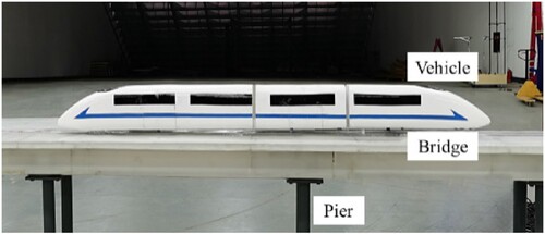
CRH3 (Xiang et al., 2022) is employed to the train model in the numerical simulation. Some details of the model are ignored to improve the mesh quality and save calculation resources. A scale of 1/20 is adopted. The reason for adopting this scale will be explained later. As shown in Figure 1, the train model has full-scale dimensions of 3.50 m (height; denoted as H) × 3.30 m (width; denoted as B). Unless otherwise specified, all dimensions in this study are full-scale dimensions. The lengths of the head, mid, and tail vehicles are 7.09H, 6.96H, and 7.09H, respectively.

Figure 1. Schematic view of computational domain. (a) Typical section of bridge, (b) typical section of tunnel, and (c) schematic view of tunnel and bridge zones.

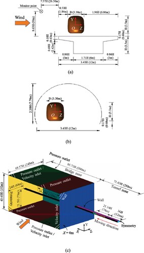
A commonly-used simply supported box girder section geometry is employed as the bridge model, as shown in Figure 1(a). The bridge with this section geometry account for a large proportion of the high-speed railway bridge in China. In addition, a typical double-track high-speed railway tunnel section geometry is employed, as shown in Figure 1(b). Meanwhile, for ease of simulating, affiliated facilities are omitted.

2.2. Computational domain and boundary conditions

The details of computational domain and boundary conditions are shown in Figure 1(c). Overall, the computational domain is divided into two parts: bridge zone and tunnel zone. Furthermore, to reduce the effect of the computational domain boundary, the blocking ratio is about 2%.

The studies by Zhou et al. (2021) and Deng et al. (2020) had proven that the variations of aerodynamic load were both significant during the processes of the train exiting and entering the bridge–tunnel sections. During the process of the train entering the tunnel, the wind speed of crosswinds and the wind loads on the train decrease. It is a process of unloading the loads. During the process of the train exiting the tunnel, the wind speed, and the wind loads increase. It is a process of applying the loads. Therefore, exiting the tunnel is more unfavourable for driving safety. Considering the saving calculation resources, the process of the train exiting the tunnel is investigated as an example in this study. Moreover, the train exiting the tunnel and then entering the bridge is defined as the train exiting the bridge–tunnel sections.

2.3. Computational grid

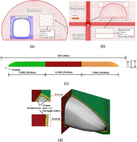
According to the study by Meng et al. (2021), the overset mesh technique has the advantages of easier mesh generation and more flexible, which has been widely employed to obtain the aerodynamic characteristics of moving train. Therefore, the overset mesh technique is employed in this work.

The static region is used as the background region, as shown in Figure 2(a,b). Meanwhile, the motion region is used as the component region, as shown in Figure 2(a). More detailed information of the overset mesh technique can be found in J. He et al. (2022). Furthermore, the number of orphan cells near overset interface is 0 during every time step of the simulation. It indicates that there is sufficient overlap between meshes and the mesh resolutions match well. In addition, the boundary layers in the tunnel and on the bridge have the same parameters. The first layer height of the tunnel and bridge is 0.002 m (5.71 × 10⁻⁴ H). Moreover, 19 layers are set in the boundary layer. To ensure the accuracy of the simulation, the meshes of the motion region are refined. The first layer height of the train is 0.001 m (2.86 × 10⁻⁴ H) and the value of y+ is less than 2 with an expansion ratio of 1.2. The grids in the motion region are shown in Figure 2(c,d).

Figure 2. Schematic view of computational mesh. (a) Cross-sectional mesh schematic of tunnel zone, (b) cross-sectional mesh schematic of bridge zone, (c) mesh side view of motion region, and (d) mesh detail of motion region.

2.4. Numerical method

The Reynolds number is about 1.6 × 10⁵ based on the height of the train. It corresponds to the Reynolds number of the wind tunnel test in Xiang et al. (2022). The turbulence model selected in the present study should be suitable for this Reynolds number. There are many turbulence models available as alternatives. The first available turbulence model is large eddy simulation (LES). Although previous study (K. He et al., 2022) had proven that LES was suitable for the simulation of a high-speed train, a high-resolution grids for wall boundary layers and a relatively small time steps were necessary. Therefore, this turbulence model is not the best choice. The second available turbulence model is shear-stress transport (SST) k-ω model (Menter, 1994). This turbulence model can save a lot of calculation resources compared with the first one and it was employed by several studies (Xia et al., 2020; Yao et al., 2020; Zou et al., 2020). Meanwhile, a low-Reynolds number correction can be adopted to suit this situation. However, the use of the low-Reynolds number terms in the k-ω models was not recommended (Liu et al., 2021). Furthermore, the more sophisticated and more widely calibrated models were advised to adopted according to the Fluent User’s Guide. In other words, the Transition SST model (Menter et al., 2006) and k-kl-ω model (Walters & Cokljat, 2008) are advised. They are the third and fourth available turbulence models, respectively. From Fluent User’s Guide, the recommended maximum value of y+ is 1 for the third model, and a wall normal expansion ratio that is less than 1.1. That is to say, the third model requires a lot of calculation resources just like the first model. While the mesh requirements of the k-kl-ω model are less stringent than that of the Transition SST model. In addition, previous study had proven that y+ < 2 can give an accurate result for the k-kl-ω model (Liu et al., 2020). This model can not only be used to effectively address the transition of the boundary layer from a laminar to a turbulent regime, but also give a good prediction for turbulence simulation (Walters & Cokljat, 2008). Therefore, the k-kl-ω model is employed in the present study.

The y+ value of the first boundary layer should be less than 2 for this model. If a full-scale model is used for simulation, the grid height of the first layer will be very small and a high-resolution grid will be required. Compared with full-scale model, scale model requires lower resolution of grid and less computational resources. It prompts the selection of a scale model in this work.

A double-precision solver recommended by Fluent User’s Guide is adopted. According to the Fluent User’s Guide, pressure-based and density-based approaches both have a broad applicable range from incompressible to highly compressible flows. The origins of the pressure-based approach may give the simulation an accuracy advantage over the density-based approach for low-speed incompressible flows. The convergence speed of the coupled algorithm is significantly faster than that of the segregated algorithm. Meanwhile, the coupled solver has a good robustness for transient simulations. Therefore, the pressure-based coupled algorithm is employed. The second-order upwind discretization scheme is selected for the equation of momentum, turbulent kinetic energy, laminar kinetic energy, and dissipation rate. Furthermore, the residuals for all parameters are 10⁻⁶. The maximum number of iterations is 40 per time step. The time step is 1 × 10⁻³ s (Zampieri et al., 2020) which is smaller than that used in the previous studies (Chen et al., 2017; Liu et al., 2017).

2.5. Data processing

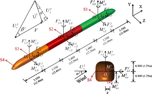
As shown in Figure 3, the sign of aerodynamic force components is regulated. Meanwhile, the relationship between the yaw angle (β^j), the velocity of the moving train (V), incoming wind speed (U^j), and wind speed relative to the train ($U_r^j$) is also shown. The superscript j serves as an indicator on whether the non-uniform airflow is adopted, i.e. j = u and j = n indicate the parameters or the calculational results are obtained under uniform and non-uniform airflows. For ease of comparison, the aerodynamic coefficients are expressed by a reference wind speed (U_r).

Figure 3. Sign convention of aerodynamic force components on the vehicle and location of the lines on the train surface.

Side force coefficient: (1) $\begin{array}{r}{C}_{S,i}^j=\frac{F_{z,i}^j}{\frac{1}{2}\rho {U_r}^{2}H{L}_i}\end{array}$(1) Lift force coefficient: (2) $\begin{array}{r}{C}_{L,i}^j=\frac{F_{y,i}^j}{\frac{1}{2}\rho {U_r}^{2}H{L}_i}\end{array}$(2) Rolling moment coefficient: (3) $\begin{array}{r}{C}_{Mx,i}^j=\frac{M_{x,i}^j}{\frac{1}{2}\rho {U_r}^2{B}^2{L}_i}\end{array}$(3) Yawing moment coefficient: (4) $\begin{array}{r}{C}_{My,i}^j=\frac{M_{y,i}^j}{\frac{1}{2}\rho {U_r}^2{B}^2{L}_i}\end{array}$(4) Pitching moment coefficient: (5) $\begin{array}{r}{C}_{Mz,i}^j=\frac{M_{z,i}^j}{\frac{1}{2}\rho {U_r}^2{B}^2{L}_i}\end{array}$(5) Overturning moment coefficient: (6) $\begin{array}{r}{C}_{t,i}^j=\frac{C_{S,i}^{j}Hy+C_{L,i}^{j}Hz+C_{Mx,i}^j{B}^2}{B^2}=\frac{M_{t,i}^j}{0.5\rho {U_r}^2{B}^2{L}_i}\end{array}$(6) Wind speed reduction coefficient: (7) $\begin{array}{r}{r}_w^j=\frac{U_z^j}{U_r}\end{array}$(7) where ρ is the air density; $F_{z,i}^j$ and $F_{y,i}^j$ are the side and lift force; $M_{x,i}^j$, $M_{y,i}^j$, $M_{z,i}^j$, and $M_{t,i}^j$ are the rolling, yawing, pitching, and overturning moment, respectively; L_i is the length of the model, respectively; the subscript i serves as an indicator on head, mid, and tail vehicle, i.e. i = 1, i = 2 and i = 3 indicates the parameters or the calculational results on the head, mid, and tail vehicle; y = 0.56 H and z = 0.21 H are the arm of the force (Xiang et al., 2022); θ is the wind direction angle.

To exhibit the flow around the train under non-uniform airflows, four lines are employed. They are intersected by cross-sectional planes in the X- and Y-directions, i.e. S1, S2, S3, and S4, as shown in Figure 3. Meanwhile, the S1, S2, and S3 represent vertical section in the middle of the head, mid, and tail vehicles. The S4 represent horizontal longitudinal sections at the centre of the train. The pressure coefficients for them can be defined as: (8) $\begin{array}{r}{C}_p=\frac{P}{\frac{1}{2}\rho {U_r}^2}\end{array}$(8) where P is the pressure on the lines.

2.6. Simulation of non-uniform flow field

2.6.1. Acquisition of wind field distribution via large-scale numerical simulation of mountain terrain

In the present study, the bridge–tunnel section connecting a bridge and a tunnel located in southwestern of China is adopted as the engineering background. To obtain the wind field distribution in the bridge–tunnel section, a large-scale numerical simulation model of mountain terrain is employed. To ensure that the experimental results are close to engineering reality, the size of the terrain model has to be large enough and the bridge site is located at the middle of the terrain model. The model with dimensions of 25 km (length) × 25 km (width) × 12 km (height) and a scale of 1/20 is employed. The computational mesh and boundary conditions of the numerical simulation are shown in Figure 4(a). The numerical simulation model is discretized by tetrahedral unstructured meshes. To ensure the calculation accuracy, the local meshes near the bridge–tunnel section are densely divided. And the number of meshes is about 4.87 million.

Figure 4. Numerical simulation model information of mountain terrain. (a) Computational mesh and boundary conditions and (b) wind profile of the velocity inlet.

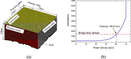
Considering that the wind speed profile with the power law exponent was used as the onset flow in wind tunnel tests of mountain terrain (Hui et al., 2009; Li et al., 2017; M. Zhang et al., 2020), an exponential wind velocity curve is used as a wind speed distribution of velocity inlet boundary in this work. In the large-scale numerical simulation of mountain terrain, the altitude of the highest peak is 5400 m. Therefore, the gradient wind level is considered to be 5400 m. The airflow above this height is uniform and the wind speed is assumed to be 50 m/s. Meanwhile, the lowest peak altitude of velocity inlet boundary is 3045 m in the mountain terrain simulation. Therefore, the wind speed varies exponentially with altitude, when the altitude is between 3045 and 5400 m. The law of wind speed with the altitude is given by Equation (9). The wind profile of the inlet wind velocity is shown in Figure 4(b). (9) $\begin{array}{r}U=\{\begin{array}{l}50,H\left(\text{Altitude}\right)>5400\\ 50\times {\left({\displaystyle \frac{H-3045}{2355}}\right)}^{0.16},5400\ge H\ge 3045\end{array}\end{array}$(9) In this mountain terrain simulation, the bridge deck altitude is 3691 m. According to Equation (9), the inlet wind velocity at the height of bridge deck is 40.65 m/s. Therefore, the reference wind speed in the mountain terrain simulation is 40.65 m/s. And the flow direction is normal to the bridge axis. Other parameters in the numerical model of mountain terrain can be found in M. Zhang et al. (2019).

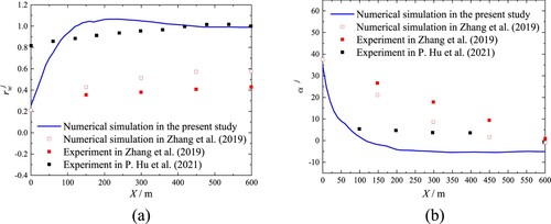
The distributions of the wind speed reduction coefficient ($r_w^j$) and wind attack angle (α^j) along the bridge longitudinal axis are shown in Figure 5 by blue solid line. The reference wind speed of blue solid line in Figure 5(a) is the inlet wind velocity at the height of bridge deck, i.e. 40.65 m/s. The symbol of X represents the position of lane. X < 0 denotes that the position is in the tunnel zone; X = 0 denotes the position of the tunnel exit; X > 0 denotes that the position is in the bridge zone. To obtain the law of wind field distribution on the bridge–tunnel section, the x-axis coordinate range of 0–600 m is employed, in Figure 5. The results in P. Hu et al. (2021) and M. Zhang et al. (2019) are also given in Figure 5. Due to different mountain terrain conditions, the results are different. However, they have some common characteristics. The airflows near the tunnel exit have the characteristics of small wind speed and large attack angle. Meanwhile, the wind field distribution far away from the tunnel exit is nearly uniform. Those also indicated that the wind field near the bridge–tunnel section has a significant non-uniformity.

Figure 5. Results of mountain terrain numerical simulation in the bridge–tunnel section along bridge longitudinal. (a) Distribution of wind speed reduction coefficients and (b) distribution of wind attack angles.

2.6.2. Velocity inlet boundary condition of non-uniform flow field

For the case of the uniform airflow simulation, the wind speed used to compute wind loads on the train model is 8 m/s (U_r). In this work, the wind load of the train with a yaw angle of 36.2° is investigated as an example. Therefore, the travelling speed of the train in the numerical simulation is set to 10.93 m/s (V).

The non-uniformity of airflows is one of the wind field distribution characteristics caused by mountainous terrain effect. The objective of this study is to evaluate the wind loads on the high-speed train under non-uniform airflow in the bridge–tunnel section. The wind field distribution is obtained by using a large-scale numerical simulation of mountain terrain in Section 2.6.1. According to wind field distribution, a user-defined function (UDF) is defined. To simulate non-uniform wind speed and attack angle, the UDF contains horizontal and vertical wind speed information. Finally, this UDF is applied to every velocity inlet boundary. To verify that the wind speed characteristics experienced by the train in this study are consistent with the boundary velocity inlet, monitor points are employed. The position of the monitor points is evenly distributed along the bridge longitudinal axis with an equal distance of 10 m, as shown in Figure 1(a). The results of the monitor points are shown in Figure 6. Considering that the focus of this work is the aerodynamic characteristics of a train under non-uniform airflows, it is unnecessary to discuss the aerodynamic characteristics under uniform airflow. Therefore, the x-axis coordinate range of 0–300 m is employed in Figure 6.

Figure 6. Results of monitor points along bridge longitudinal axis. (a) Distribution of wind speed reduction coefficients and (b) distribution of wind attack angles.

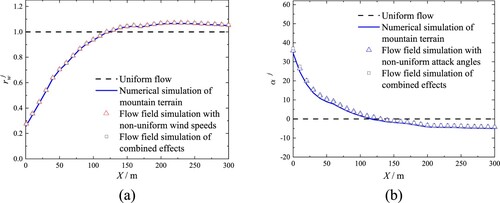
For the case of the airflow simulation with non-uniform wind speeds, only the wind speeds at the velocity inlet along the bridge longitudinal axis are varied. The value of reference wind speed (U_r) is 8 m/s. Meanwhile, the wind attack angles are 0°. The boundary conditions of the top and bottom surface are pressure outlet. Moreover, the wind speed reduction coefficient results of the monitor points are shown in Figure 6(a) by red triangles. For the case of the airflow simulation with non-uniform wind attack angles, only the wind attack angles along the bridge longitudinal axis are varied according to the rule in Figure 6(b). Meanwhile, the incoming wind speeds are not varied and equal to 8 m/s. To realise the simulation of the non-uniform wind attack angles airflows, the boundary conditions of the top and bottom surface are modified. From Figure 6(b), the sign of wind attack angle reverses from positive to negative at about X = 34.29H (120 m). Therefore, the boundary conditions of the top and bottom surface at the range of X > 34.29H are modified to velocity inlet and pressure outlet, respectively. Those at the range of 0 < X < 34.29H are modified to pressure outlet and velocity inlet, respectively, as shown in Figure 1(c). In addition, the results of the monitor points are shown in Figure 6(b) by blue triangles. For the simulation of combined effects, the wind speeds and wind attack angles are synchronously modified according to the rule in Figure 6. The boundary condition modification of combined simulation is similar to that of the separate simulation. In addition, the results of the monitor points are shown in Figure 6 by black squares. The wind field distribution experienced by the monitor points is consistent with that at the velocity inlet. It indicates that the non-uniform characteristics of wind speed and attack angle in the numerical simulation model are simulated successfully.

3. Verification of bridge–tunnel section model

3.1. Independence verification of residual value

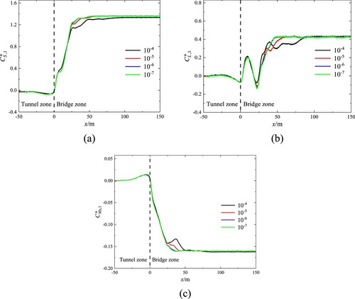
To select a suitable residual, the residual values of 10⁻⁴, 10⁻⁵, 10⁻⁶, and 10⁻⁷ are compared in the present study. In this section, the results of the head vehicle are investigated as examples. The results for the four residual values are shown in Figure 7, in which x denotes the nose tip position of the head vehicle. x < 0 denotes that the nose tip of the head vehicle is in the tunnel zone; x = 0 denotes that the nose tip reaches the tunnel exit; x > 0 denotes that the nose tip is in the bridge zone. It should be noted that the vibration of aerodynamic coefficients decreases as the residual value decreases. Meanwhile, the simulation results with the residual value of 10⁻⁶ and 10⁻⁷ are almost the same, which indicates that the residual values of 10⁻⁶ is small enough for the simulation in this work.

Figure 7. Results for different residual values. (a) Side force coefficient, (b) lift force coefficient, and (c) rolling moment coefficient.

3.2. Grid independence

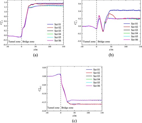
To verify the independence of the computational grid, four sets of grids are employed. Considering that the mesh around the train plays an important role in the results, only the mesh in the motion region is changed and the mesh in static region is not changed in the verification. The grid number of the four sets is shown in Table 1.

Table 1. Grid configuration in the grid independence verification.

		Motion region				Static region
		Min value of element profile length				Min value of element profile length
	Element number (million)	X-axis	Y-axis	Z-axis	Element number (million)	X-axis	Y-axis	Z-axis
Set 01	0.95	4.40 × 10^−4H	1.51 × 10^−4H	2.94 × 10^−4H	4.53	5.71 × 10^−3H	6.29 × 10^−4H	3.43 × 10^−3H
Set 02	3.00	3.11 × 10^−4H	1.49 × 10^−4H	1.74 × 10^−4H
Set 03	4.03	2.83 × 10^−4H	1.40 × 10^−4H	1.69 × 10^−4H
Set 04	5.01	2.76 × 10^−4H	1.39 × 10^−4H	1.63 × 10^−4H
Set 05	4.03	2.83 × 10^−4H	1.40 × 10^−4H	1.69 × 10^−4H	6.64	3.43 × 10^−3H	5.71 × 10^−4H	1.70 × 10^−3H
Set 06					10.23	1.71 × 10^−3H	1.12 × 10^−4H	1.51 × 10^−3H

Taking the aerodynamic coefficients of the head vehicle as examples, the results for different grid settings are shown in Figure 8. The results of the Set 03 and 04 are very close. It indicates that the mesh resolution of the motion region in Set 03 is high enough for the simulation. The results of the Set 03, 05, and 06 are very close. It indicates that the mesh resolution of the static region in Set 03 is high enough for the simulation.

Figure 8. Results for different grid settings. (a) Side force coefficient, (b) lift force coefficient, and (c) rolling moment coefficient.

3.3. Comparison with experimental results

To verify the accuracy of the numerical model comprehensively, it is necessary to compare the simulation results with experiment results. A wind tunnel test is conducted in the XNJD-3 wind tunnel at Southwest Jiaotong University in China, as shown in Figure 9. The test wind speed was set to 8 m/s (Xiang et al., 2022). The scale of 1/20 is adopted in this test. To ensure that the verification of the numerical simulation is convincing in this section, the same scale as the wind tunnel test is adopted by the numerical simulation. And the wind speed of 8 m/s is employed to simulate the aerodynamic characteristics of the high-speed train under uniform airflow. Therefore, the value of reference wind speed is 8 m/s in obtaining train aerodynamic characteristics under non-uniform airflow.

Figure 9. Photograph of train model in wind tunnel test.

To compare the simulation results with experiment results, a static test is employed and the results are shown in Table 2. For the side force coefficient, the maximum percentage error is less than 10%. And the percentage errors of the overturning moment coefficients are approximately 10%. However, the percentage errors of lift force and rolling moment coefficient are more than 10%. In terms of rolling moment coefficient, although the percentage error is relatively large, the absolute values of results are slight and the absolute errors are also slight. For the lift force coefficient, the error may be caused by two aspects. First, the surface of the geometric model in the numerical simulation is smoother than that in the wind tunnel test. Second, the bridge deck is not completely flat in the test. It leads to the distance error between the train bottom and the bridge deck. Overall, the agreement between the test results and numerical simulation results is deemed adequate.

Table 2. Comparison between the wind tunnel test and simulation.

	Aerodynamic coefficients	Experiment	Simulation	Absolute of error	Percentage error (%)
Head vehicle	$C_{S,1}^u$	0.855	0.822	0.033	4%
	$C_{L,1}^u$	0.388	0.281	0.107	28%
	$C_{Mx,1}^u$	−0.081	−0.091	0.010	−12%
	$C_{t,1}^u$	0.549	0.493	0.056	10%
Mid vehicle	$C_{S,2}^u$	1.155	1.050	0.105	9%
	$C_{L,2}^u$	0.308	0.360	0.053	17%
	$C_{Mx,2}^u$	−0.077	−0.094	0.017	−22%
	$C_{t,2}^u$	0.723	0.652	0.071	10%

4. Results and discussion

The wind field distribution in the bridge–tunnel section is mainly shown as the non-uniform characteristics of wind speed, wind attack angle, and wind direction angle. Considering that the aerodynamic characteristics under crosswinds are unfavourable (X. Li et al., 2021), the direction of wind is normal to that of train motion.

Due to effects of mountains, the distributions of wind speeds and attack angles along the bridge longitudinal axis are non-uniform (see Figure 5). Meanwhile, the studies of the single factor effects are the foundation of that of the combined effects. Therefore, it is necessary to discuss the effect of single factor on the resultant aerodynamic characteristics. To understand the aerodynamic characteristics of the train under non-uniform airflows comprehensively, the aerodynamic loads and flow features are discussed in this section.

4.1. Effects of non-uniform wind speeds

Previous studies (Deng et al., 2020; Yang et al., 2020) had shown that the head vehicle had the highest wind load compared with the middle and tail vehicles when the train travelled on a bridge–tunnel section under crosswinds. Meanwhile, Zhou et al. (2021) had proven that the head vehicle was severely affected during these processes. They also proved that the aerodynamic coefficient peak–peak value of the head vehicle was the highest. There is a reason to believe that the head vehicle has the largest wind loads during this process. Considering the limitations of space, the head vehicle was adopted as an example in this section.

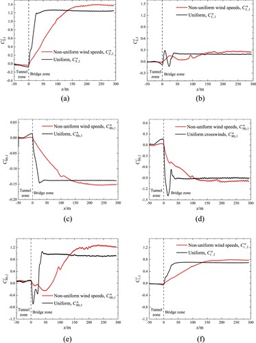
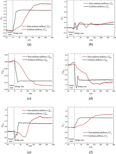
The time histories of the aerodynamic coefficients under uniform airflows and non-uniform wind speeds airflows in the bridge–tunnel section are illustrated in Figure 10. The solid black line indicates the aerodynamic coefficients under uniform airflows, and the solid red line indicates the aerodynamic coefficients under non-uniform wind speeds airflows. All the aerodynamic coefficients have a significant sudden change in the process under uniform airflows. The aerodynamic coefficients are almost equal to 0 when the head vehicle runs in the tunnel. Then, the absolute value of the aerodynamic coefficients increases with the vehicle movement. It reaches its peak when the nose tip of the vehicle approaches the tunnel exit. The peak values under uniform airflows are greater than those under non-uniform airflows. After that, the aerodynamic coefficients quickly change from positive to negative or vice versa and reach a noticeable value. It is noted that the slope absolute values of the aerodynamic coefficients to the distance under uniform airflows are greater than those under non-uniform wind speeds airflows near the tunnel exit, as shown in Figure 10. The reason is that the differences of the wind speed between inside and outside the tunnel under non-uniform airflows are smaller than those under uniform airflow. When 0 ≤ x ≤ 24.8 m, the wind loads of the train under uniform airflows reaches an appreciable level. However, under non-uniform wind speeds airflows, the maximum values of side force, lift force, rolling moment, yawing moment, pitching moment, and overturning moment coefficients are decreased by 78%, 48%, 75%, 64%, 88%, and 72%, respectively. It is beneficial for driving safety. When x ≥ 225 m, the wind loads of the train under non-uniform airflows are greater than those under uniform airflows. More specifically, the mean wind speed far away from the tunnel exit under non-uniform airflows is increased by 6.6% comparing with that under uniform airflows. The mean side force, lift force, rolling moment, yawing moment, pitching moment, and overturning moment coefficients of the head vehicle are increased by 11.5%, 36.3%, 10.3%, 9.7%, 36.2%, and 13.4%, respectively. It is detrimental to driving safety.

Figure 10. Aerodynamic coefficients of the head vehicle under uniform airflows and non-uniform wind speeds airflows. (a) $C_{S,1}^j$, (b) $C_{L,1}^j$, (c) $C_{Mx,1}^j$, (d) $C_{My,1}^j$, (e) $C_{Mz,1}^j$, and (f) $C_{t,1}^j$.

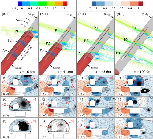
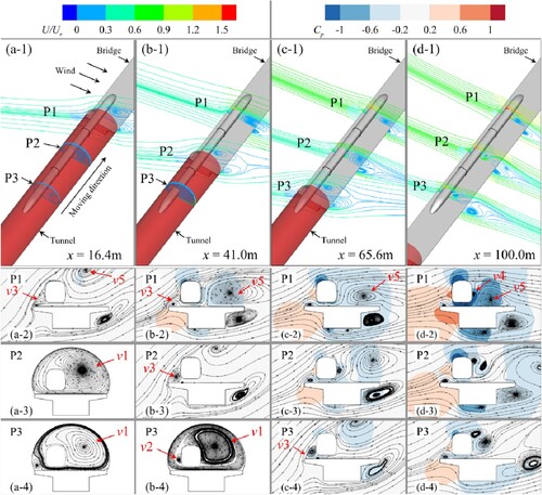
To reveal the differences of the transient flow field and the mechanism of the aerodynamic load under uniform and non-uniform airflows, the transverse slice diagrams of the streamline structure at different positions are shown in Figure 11. x = 16.4 m (4.69H), 41.0 m (11.71H), and 65.6 m (18.74H) correspond the moments that the distance along the vehicle longitudinal axis between the tunnel exit and the key section of S1, S2, and S3 are both 4.0 m (1.14H). x = 100.0 m (28.57H) corresponds the moment that the train far away from the tunnel exit. Moreover, the P1, P2, and P3 represent the section of the flow field at the positions of the S1, S2, and S3, respectively. Furthermore, the streamlines in Figure 11 are coloured by the dimensionless wind speed of U/U_r, where U is the 3D combined wind speed.

Figure 11. Flow field characteristics in the bridge–tunnel section. (a) Under uniform airflows and (b) under non-uniform wind speeds airflows.

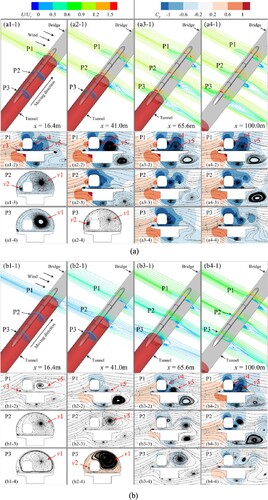
The vortex structure and pressure distribution around the train at different positions are shown in Figure 11. When the train is in the tunnel, the vortex structures of v1 and v2 are formed. However, the wind speeds around the train are small. The size of v2 under uniform airflows is larger than that under non-uniform airflows. It is the effect of wind speed near the tunnel exit. The size of v2 is decreased with the decrease of wind speed near the tunnel exit. It causes that the peak of wind load under uniform airflows is higher than that under non-uniform airflows when x is approximately 0 m, as shown in Figure 10. From Figure 11(a), the vortex structure of v3 is formed on the vehicle windward side and the vortex structures of v4 and v5 are formed on the vehicle leeward side when the vehicle runs on the bridge under uniform airflows. The vortex v3 does not changed with the movement of the train. Because it is formed by the separation of airflow at the windward edge of the bridge. The vortices v4 and v5 changed with the movement of the train. Their size rapidly increases when the train travels near the tunnel exit. And it remains unchanged when the train is away from the exit. The pressure coefficients around the train and bridge do not change much.

Whether uniform or non-uniform wind speeds airflows is applied to the head vehicle, the vortices v3, v4, and v5 are formed around the vehicle. However, there is a difference in the timing of the vortex formation. From Figure 11(b1–4), when the vehicle leaves the tunnel under the non-uniform wind speeds airflows, v4 is not immediately formed, while only a large-sized vortex v5 is formed. This precisely corresponds to the fact that the slope absolute value of the aerodynamic coefficients has a low level after leaving the tunnel in Figure 10. Meanwhile, the pressure coefficient distribution around the train and bridge varies at different sections.

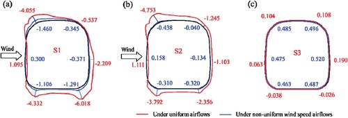
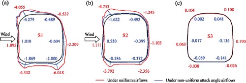
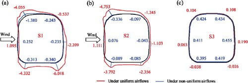
To further reveal the flow features around train, the distributions of the pressure coefficients for the S1, S2, and S3 are investigated shown in Figure 12. A positive pressure area on the train windward surface and negative pressure areas on the rest surface are formed in Figure 12(a,b). Moreover, the absolute values of the negative pressure on the windward roof and base corner are higher than the rest surface of the roof, underbody and leeward side. Those are consistent with the results of previous investigation in Wang et al. (2018). The difference of pressure coefficients between the S1 and S2 under non-uniform airflows is smaller than that under uniform airflows. Therefore, when the train runs near the tunnel exit, the variation of the absolute values of the aerodynamic coefficients under non-uniform airflows is less significant compared with that under uniform airflows. From Figure 12(c), the pressure coefficient distribution for the S3 is symmetrical. The reason is that the pressure at the section in tunnel is affected by the pressure waves. It indicates that non-uniform wind speeds flow has little effect on the aerodynamic coefficients of the train in the tunnel. This is consistent with the results of previous investigations in Deng et al. (2020). In addition, the absolute values of pressure coefficient for the S3 under uniform airflows are smaller than that under non-uniform airflows. The reason may be that the pressure waves is reduced by the crosswinds near the tunnel exit and the reduction effect increases as the wind speeds increases.

Figure 12. Distributions of the pressure coefficients for the S1, S2, and S3 (x = 41.0 m).

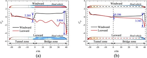
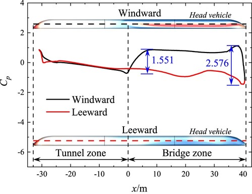
The distributions of the pressure coefficients for the S4 under uniform airflows and non-uniform airflows are shown in Figure 13. The maximum pressure coefficients difference between the windward and leeward for the S4 is 5.804 under uniform airflows, and that is 3.343 under non-uniform airflows. The sudden change of the pressure coefficient difference near the tunnel exit is 2.205 under uniform airflows, and that is 0.186 under the non-uniform airflows. The pressure coefficient difference between the windward and leeward along the vehicle longitudinal axis in the tunnel is small.

Figure 13. Distributions of the pressure coefficients for the S4 (x = 41.0 m). (a) Under uniform airflows and (b) under non-uniform wind speeds airflows.

4.2. Effects of non-uniform wind attack angles

The time histories of the aerodynamic coefficients under uniform airflows and non-uniform wind attack angles airflows in the bridge–tunnel section are illustrated in Figure 14. The solid black line indicates the aerodynamic coefficients under uniform airflows, and the solid red line indicates the aerodynamic coefficients under non-uniform wind attack angles airflows. There are two characteristics of the aerodynamic coefficients of the vehicle under non-uniform wind attack angles airflows, similar to that under non-uniform wind speeds airflows. First, the slope absolute values of the aerodynamic coefficients to the distance under uniform airflows are greater than that under non-uniform airflows near the tunnel exit. Second, the aerodynamic coefficients under uniform airflows are smaller than that under non-uniform airflows when the vehicle nose tip is far away from the tunnel exit except for the lift force coefficient. When 0 ≤ x ≤ 24.8 m, the maximum values of side force, rolling moment, yawing moment, pitching moment, and overturning moment coefficients are decreased by 86%, 87%, 73%, 61%, and 68%, respectively. The maximum values of lift force coefficient are increased by 48%. When x ≥ 225 m, the wind attack angles under the non-uniform airflows are about −5°. The mean value of side force, rolling moment, yawing moment, pitching moment, and overturning moment coefficients under non-uniform wind attack angles airflows increase by 21.6%, 7.2%, 14.4%, 58.3%, and 22.1%. The mean value of lift force coefficient shows reduction of 15.8%. During the process of movement, the peak values of the pitching moment coefficients under non-uniform wind attack angles airflows are greater than that under uniform airflows in Figure 14(e). The reason is that the distribution of lift force fluctuates is great, as shown in Figure 14(b).

Figure 14. Aerodynamic coefficients under uniform airflows and non-uniform wind attack angles airflows. (a) $C_{S,1}^j$, (b) $C_{L,1}^j$, (c) $C_{Mx,1}^j$, (d) $C_{My,1}^j$, (e) $C_{Mz,1}^j$, and (f) $C_{t,1}^j$.

The streamlines around the train under non-uniform wind attack angles airflows are shown in Figure 15. From Figure 15, it can be seen that the non-uniform wind attack angles airflows have little effect on the aerodynamic coefficients of the train and streamline structure around the train in the tunnel. Compared with the uniform airflow simulation, the non-uniform airflow simulation has a high wind attack angle near the tunnel exit. It causes a larger size of vortex v3, as shown in Figure 15(a-2,b-3,c-4). The spatial size of v3 decreases with the decrease of wind attack angle. Due to the large attack angle, the vehicle is in the wake of the bridge. This leads the airflow separation points on the vehicle surface to be close to the windward side. Meanwhile, small-sized vortex v6 and large-sized v5 are formed, as shown in Figure 15(a-2). The vortex v6 disappears with the movement of the vehicle, while the vortex v4 is formed on the leeward side of the vehicle and its size continues to be increased. It also can be seen that the bridge has a shelter effect on the vehicle when the vehicle travels near the tunnel exit. These results in a lower level of the slope absolute value of the aerodynamic coefficient under non-uniform wind attack angles airflows compared with that under uniform airflows. The disappearance and formation of the vortices leads to a significant fluctuation amplitude of the lift coefficient near the tunnel exit.

Figure 15. Flow field characteristics when the train moves in the bridge–tunnel section under non-uniform wind attack angles airflows.

The distributions of the pressure coefficients for the S1, S2, and S3 under uniform and non-uniform wind attack angles airflows are shown in Figure 16. The distributions of the positive and negative pressure areas for the S1 and S2 under non-uniform airflows are similar to those under uniform airflows, as shown in Figure 16. However, the absolute values of the pressure coefficients of the former are smaller than those of the latter except for that on the windward roof for the S1. In addition, due to the formations of the vortex structure of v3 and v5 near the tunnel exit, the pressure coefficients differences for the S2 between the windward and leeward surface under non-uniform airflows are smaller than those under uniform airflows. Meanwhile, the differences between the top and bottom surface under the former are also smaller than those under the latter. As a result, the slope absolute values of the aerodynamic coefficients near the tunnel exit under non-uniform airflows are smaller than the corresponding values under uniform airflows.

Figure 16. Distributions of the pressure coefficients for the S1, S2, and S3 under non-uniform wind attack angles airflows (x = 41.0 m).

The distributions of the pressure coefficients for the S4 under non-uniform airflows are shown in Figure 17. The maximum pressure coefficients difference between the windward and leeward under non-uniform airflows is 2.576 which is smaller than that under uniform airflows. Meanwhile, the sudden change of the pressure coefficient on the train windward side near the tunnel exit under non-uniform airflows is 1.551. The slope of the pressure coefficient to the distance under non-uniform airflows is smaller than that under uniform airflows. The pressure coefficient on the train leeward side changes unremarkably.

Figure 17. Distributions of the pressure coefficients for the S4 under non-uniform wind attack angles airflows (x = 41.0 m).

4.3. Combined effects of non-uniform wind speeds and wind attack angles

The time histories of the aerodynamic coefficients under uniform and non-uniform airflows in the bridge–tunnel section are illustrated in Figure 18. The solid black line indicates the aerodynamic coefficients under uniform airflows, and the solid red line indicates the aerodynamic coefficients under non-uniform airflows. Compared with the two cases mentioned above, the slope absolute values of the aerodynamic coefficients under uniform airflows are the smallest, when the vehicle travels near the tunnel exit. It slows down sudden change of the aerodynamic characteristics of the train. Meanwhile, the aerodynamic coefficients are the greatest, when the vehicle travels far away from the tunnel exit. When 0 ≤ x ≤ 24.8 m, the maximum values of side force, lift force, rolling moment, yawing moment, pitching moment, and overturning moment coefficients are decreased by 92%, 65%, 95%, 87%, 93% and 86%, respectively. When x ≥ 225 m, the mean side force, lift force, rolling moment, yawing moment, pitching moment, and overturning moment coefficients are increased by 33.4%, 37.9%, 23.4%, 18.8%, 70.7%, and 35.7%, respectively.

Figure 18. Aerodynamic coefficients under uniform airflows and non-uniform airflows. (a) $C_{S,1}^j$, (b) $C_{L,1}^j$, (c) $C_{Mx,1}^j$, (d) $C_{My,1}^j$, (e) $C_{Mz,1}^j$, and (f) $C_{t,1}^j$.

The streamlines of the combined effects around the train are shown in Figure 19. From Figure 19, it can be seen that non-uniform airflows have little effect on the streamline structure around train and aerodynamic coefficients of train when the train travels in the tunnel. The formation position of vortices v4 and v5 around the train is further behind. Compared with the two situations mentioned above, the slope absolute values of the aerodynamic coefficients under non-uniform airflows are smallest. It takes a long time for the aerodynamic coefficients of the train to reach the maximum value. It is beneficial for the driving safety. From Figures 15 and 19, the streamline structure around the train under non-uniform airflows is not significantly different from that under non-uniform wind attack angles airflows when x ≤ 41 m. From Figures 11(b) and 19, the streamline structure under non-uniform airflows is not significantly different from that under non-uniform wind speeds airflows when x = 100 m. It indicates that the non-uniform wind attack angle effect plays an important role in the streamline structure when the train travels near the tunnel exit. Meanwhile, the non-uniform wind speed effect plays an important role when the train travels far from the tunnel exit.

Figure 19. Flow field characteristics when the train moves in a bridge–tunnel section under non-uniform wind speeds and attack angles airflows.

The distributions of the pressure coefficients for the S1, S2, and S3 under uniform and non-uniform airflows are shown in Figure 20. The distributions of the positive and negative pressure areas under non-uniform airflows are similar to that under uniform airflows, as shown in Figure 20, except for the S3. The absolute values of the pressure coefficients under non-uniform airflows are smaller. In addition, due to the combined effects of the non-uniform wind speed and wind attack angle, the pressure coefficients differences between the windward and leeward surface are smallest for the S2, compared with the two situations mentioned above. The differences between the top and bottom surface are also smallest. It causes the slope absolute values of the aerodynamic coefficients near the tunnel exit under non-uniform airflows are smallest.

Figure 20. Distributions of the pressure coefficients for the S1, S2, and S3 under non-uniform wind speeds and attack angles airflows (x = 41.0 m).

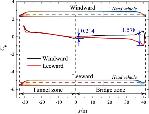
The distributions of the pressure coefficients for the S4 are shown in Figure 21. Compared with the other three cases, the maximum pressure coefficients difference between the windward and leeward for the S4 in this case is 1.578 which is the smallest. The sudden change of the pressure coefficient on the train windward side for the S4 near the tunnel exit is 0.214. And the pressure coefficient on the train leeward side for the S4 changes unremarkably. The sudden change of the pressure coefficient difference near the tunnel exit under the combined effects is close to that under the non-uniform wind speeds airflows. Therefore, it indicates that the sudden change of the pressure coefficient difference near the tunnel exit is greatly affected by the wind speeds.

Figure 21. Distributions of the pressure coefficients for the S4 under non-uniform wind speeds and attack angles airflows (x = 41.0 m).

4.4. Approximate calculation of aerodynamic coefficients of the train

The aerodynamic coefficients in the bridge–tunnel section are affected by non-uniform airflows. In practice, it is time consuming to obtain the aerodynamic coefficients by CFD, especially 3D numerical simulation. Considering that the overturning moment coefficient is important for evaluating vehicle safety (Xiang et al., 2022), an approach is proposed to predict the coefficient under non-uniform airflows in this section.

To achieve this, two parameters are employed. The first parameter is the reduction coefficient of wind speed ($r_w^j$), which is used to quantify the aerodynamic characteristics relationship between uniform airflows with the wind speed of 8 m/s and non-uniform airflows with variable wind speeds. The second parameter is the coefficient of wind attack angle ($r_{\alpha }^u$), which is used to quantify the aerodynamic characteristics relationship between the uniform airflows with the wind attack angle of 0° and that of α.

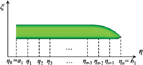
For ease of explaining, the overturning moment coefficients of head vehicle are investigated as examples. The local coordinate system of the vehicle is shown in Figure 22. $c_{\alpha }^j\left(\eta \right)$ denotes the value of the vehicle overturning moment coefficient per unit length with a wind attack angle of α at a section of η. j = u and j = n separately indicates the parameters obtained under uniform and non-uniform airflows. The overturning moment coefficient of the head vehicle under uniform airflows with a wind attack angle of 0° can be defined as: (10) $\begin{array}{r}{M}_{t,1}^u={\int }_{a_1}^{b_1}\frac{1}{2}\rho B{\left(U_z^u\right)}^2{c}_0^u\left(\eta \right)d\eta \end{array}$(10) where $U_z^u$ denotes the wind speed of the uniform airflows and its value is equal to the reference wind speed (U_r) in the present study; b₁ and a₁ denote the position of the nose tip and end of head vehicle, as shown in Figure 22.

Figure 22. Local coordinate system of the vehicle.

Note that the head vehicle overturning moment coefficient can also be deduced from Equation (10) as: (11) $\begin{array}{r}{C}_{t,1}^u=\left({\int }_{a_1}^{b_1}{c}_0^u\left(\eta \right)d\eta \right)/L_1\end{array}$(11) where L₁ is the length of the head vehicle.

Similarly, the overturning moment coefficient of the head vehicle under non-uniform airflows can be defined as: (12) $\begin{array}{r}{M}_{t,1}^n={\int }_{a_1}^{b_1}\frac{1}{2}\rho B{\left[U_z^n\left(\eta \right)\right]}^2{c}_{\alpha }^n\left(\eta \right)d\eta \end{array}$(12) where $U_z^n\left(\eta \right)$ denotes the wind speed of the non-uniform airflows along the head vehicle longitudinal axis. According to Equation (7), the wind speed of the non-uniform airflows ($U_z^n\left(\eta \right)$) can be expressed by the wind speed of the uniform airflows ($U_z^u$) and the reduction coefficient of wind speed ($r_w^n\left(\eta \right)$), as shown below: (13) $\begin{array}{r}{U}_z^n\left(\eta \right)=U_z^u{r}_w^n\left(\eta \right)\end{array}$(13)

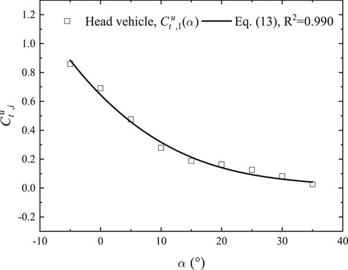
Considering that the overturning moment coefficient will be affected by the wind attack angle, it is necessary to obtain the overturning moment coefficients of train under uniform airflows with different attack angles. To meet it, the model obtaining aerodynamic characteristics is employed. The background and component regions constitute this model. Their relative positions can be changed freely as needed. In other words, the starting point of the train model movement can be located in the tunnel zone or bridge zone arbitrarily. It promotes the advancement of this task. The process of dealing with the overturning moment coefficients can be roughly divided into three steps. First, the train model is moved to the bridge zone and the computing parameters is set in Fluent; Second, the aerodynamic characteristics of the train with different attack angles is simulated; Finally, the overturning moment coefficients are fitted by Equation (14). The overturning moment coefficients of the head vehicle with different attack angles are calculated in the present study in Figure 23 and the fitting result is shown in Figure 23. Although there is no wind barrier on the bridge in this work, the bridge has the same shelter effect as the wind barrier under large wind attack angles. The shelter effect of bridge becomes decreasingly significant with the wind attack angle decrease. Therefore, the overturning moment coefficients of head vehicle decrease with the value of α increase. The coefficients A₁, A₂, A₃, and A₄ are calculated by least square method. The parameter ‘adjusted R²’ shows the fitting accuracy in Figure 23. Equation (14) can predict the overturning moment coefficients at any given wind attack angle of α. (14) $\begin{array}{rl}{C}_{t,1}^u\left(\alpha \right)& =(A_1{\alpha }^1+A_2{\alpha }^2+A_3{\alpha }^3+A_4)\cdot C_{t,1}^u\left(0\right)\\ & =r_{\alpha }^u\cdot C_{t,1}^u\left(0\right)\end{array}$(14) where $C_{t,1}^u\left(\alpha \right)$ denotes the overturning moment coefficients of the head vehicle under uniform airflows with the wind attack angle of α.

Figure 23. Overturning moment coefficients of head vehicle with different attack angles.

According to Equation (14), the relationship between the overturning moment coefficient per unit length under uniform airflows with a wind attack angle of α ($c_{\alpha }^u\left(\eta \right)$) and that of 0° ($c_0^u\left(\eta \right)$) can be assumed as: (15) $\begin{array}{r}{c}_{\alpha }^u\left(\eta \right)=r_{\alpha }^u\left(\eta \right)c_0^u\left(\eta \right).\end{array}$(15) When the wind speed and wind attack angle are fixed, the aerodynamic coefficients per unit length of each vehicle section are determined by the section geometry. Therefore, the assumption that the overturning moment coefficient per unit length under uniform airflows ($c_{\alpha }^u\left(\eta \right)$) is equal to that under non-uniform airflows ($c_{\alpha }^n\left(\eta \right)$) is reasonable. The overturning moment coefficient per unit length under non-uniform airflows ($c_{\alpha }^n\left(\eta \right)$) can be expressed by the coefficient of wind attack angle ($r_{\alpha }^u\left(\eta \right)$) and the overturning moment coefficient per unit length under uniform airflows with a wind attack angle of 0° ($c_0^u\left(\eta \right)$), as shown below: (16) $\begin{array}{r}{c}_{\alpha }^n\left(\eta \right)=r_{\alpha }^u\left(\eta \right)c_0^u\left(\eta \right).\end{array}$(16)

According to Equations (13) and (16), the overturning moment coefficient of the head vehicle under non-uniform airflows can be deduced from Equation (12) as: (17) $\begin{array}{r}{M}_{t,1}^n=\frac{1}{2}\rho B{\int }_{a_1}^{b_1}{\left[U_z^u{r}_w^n\left(\eta \right)\right]}^2{r}_{\alpha }^u\left(\eta \right)c_0^u\left(\eta \right)d\eta .\end{array}$(17) From Figure 5, the value of $[r_w^n\left(\eta \right){]}^2$ increases as the value of η increases. Moreover, the value of α decreases as the value of η increases. The value of $r_{\alpha }^u\left(\eta \right)$ increases as the value of α decreases, as shown in Figure 23. Therefore, the value of $r_{\alpha }^u\left(\eta \right)$ increases as the value of η increases. From previous study (X. Li et al., 2021), the value of $c_{\alpha }^j\left(\eta \right)$ under crosswinds is positive, i.e. $c_{\alpha }^j\left(\eta \right)>0$. Considering the above characteristics of the three parameters, the following relation can be deduced from Equation (17) as: (18) $\begin{array}{rl}{M}_{t,1}^n& \le \frac{1}{2}\rho B(U_z^u{)}^2{\int }_{a_1}^{b_1}{\left[r_w^n\left(b_1\right)\right]}^2{r}_{\alpha }^u\left(b_1\right)c_0^u\left(x\right)dx\\ & =[r_w^n\left(b_1\right){]}^2{r}_{\alpha }^u\left(b_1\right)\cdot \frac{1}{2}\rho B(U_z^u{)}^2{\int }_{a_1}^{b_1}{c}_0^u\left(x\right)dx\\ & =[r_w^n\left(b_1\right){]}^2{r}_{\alpha }^u\left(b_1\right)M_{t,1}^u.\end{array}$(18)

In consideration of driving safety, the overturning moment coefficient of the head vehicle under non-uniform airflows can be defined as: (19) $\begin{array}{r}{M}_{t,1}^n=[r_w^n\left(b_1\right){]}^2{r}_{\alpha }^u\left(b_1\right)M_{t,1}^u.\end{array}$(19) Furthermore, a more applicable equation for the head, mid, and tail vehicles can be obtained as: (20) $\begin{array}{r}{M}_{t,i}^n=[r_w^n\left(b_i\right){]}^2{r}_{\alpha }^u\left(b_i\right)M_{t,i}^u.\end{array}$(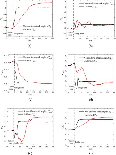20) where b_i denotes coordinate of the vehicle beginning position; i = 1, i = 2, and i = 3 are respectively represent the head, mid and tail vehicles. In Figure 24, the numerical simulation and approximate calculation results are shown. As mentioned above, the overturning moment coefficients in the tunnel are small and close to 0. Therefore, the coefficients in the tunnel are ignored. In Figure 24(b,c), CFD results show local peak when x < 150 m. This is because the wind attack angle experienced by the train is not a constant and the vortex structures are greatly affected by the wind attack angles. Meanwhile, the change of wind attack angle results in the generation and separation of the vortexes on the leeward side of the train. To quantify the accuracy of the predictions, the maximum absolute errors are given in Table 3. It indicates that the predictions via Equation (20) are in consistent with the numerical simulation results. Previous studies (Hu et al., 2021; M. Zhang et al., 2019) had shown that the airflows near the tunnel exit had the characteristics of small wind speed and large attack angle. The variation law of wind speed and wind attack angle along the bridge longitudinal in their study is consistent with that in this work. Therefore, there is a reason to believe that the equation has a certain applicability. Furthermore, the similar equations can be obtained by using the same method for different wind field distributions.

Figure 24. Results of numerical simulation and approximate calculation. (a) Results under non-uniform wind speeds airflows, (b) results under non-uniform wind attack angles airflows, and (c) results under non-uniform wind speeds and wind attack angles airflows.

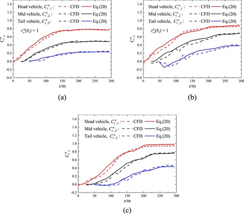
Table 3. Maximum absolute errors between numerical simulation and approximate calculation results.

Case	Head vehicle, $C_{t,1}^n$	Mid vehicle, $C_{t,2}^n$	Tail vehicle, $C_{t,3}^n$
Under non-uniform wind speeds airflows	0.065	0.040	0.067
Under non-uniform wind attack angles airflows	0.108	0.113	0.103
Under non-uniform wind speeds and wind attack angles airflows	0.102	0.088	0.077

From Equation (20), there is a good correlation between the aerodynamic characteristics and the two parameters of the wind speed reduction and wind attack angle coefficients. Therefore, the two parameters can be utilised to calculate aerodynamic characteristics under non-uniform airflows, which can simplify the calculation conditions and save calculation resources.

5. Conclusions

This paper pertains the first study on investigating the aerodynamic characteristics of a high-speed train travelling through a bridge–tunnel section under non-uniform airflows in mountainous area based on CFD. To achieve this, two numerical simulation models are employed. The first model is employed to obtain the wind field distribution in a bridge–tunnel section. The second model is employed to obtain the aerodynamic characteristics. Meanwhile, the effects of the non-uniform wind speeds and wind attack angles airflows on the aerodynamic loads and flow feature are investigated. Finally, a derived empirical equation is introduced to predict the aerodynamic coefficients of the train under non-uniform airflows caused by the mountain terrain. The following conclusions can be obtained from this work.

1. The aerodynamic characteristics of the train under non-uniform airflow caused by mountain terrain effect are quite different from those under uniform airflow. It is necessary to consider the non-uniform airflows for obtaining the aerodynamic characteristics of the train travelling through a bridge–tunnel section.

2. Due to the effects of non-uniform airflows, the aerodynamic coefficients increase slowly when the vehicle travels near the tunnel exit. It is beneficial to the driving safety. However, the coefficients have high levels when the vehicle travels far from the tunnel exit.

3. The non-uniform airflows reduce the pressure on the train surface and the jumping property of the pressure along the vehicle longitudinal axis when the train runs near the tunnel exit. And the non-uniform wind speed effect plays an important role.

4. The predictions of the overturning moment coefficients via a simple empirical equation are in the good agreement with the numerical simulation results. The calculation of the coefficients under non-uniform airflows can be simplified by using the results under uniform airflows, the wind speed reduction and wind attack angle coefficients.

Disclosure statement

No potential conflict of interest was reported by the author(s).

Additional information

Funding

The authors are grateful for the financial support from the National Natural Science Foundation of China (Grant numbers 51978589).

References

- Baker, C. J., Jones, J., Lopez-Calleja, F., & Munday, J. (2004). Measurements of the cross wind forces on trains. Journal of Wind Engineering and Industrial Aerodynamics, 92(7–8), 547–563. https://doi.org/10.1016/j.jweia.2004.03.002
- Broniszewski, J., & Piechna, J. (2019). A fully coupled analysis of unsteady aerodynamics impact on vehicle dynamics during braking. Engineering Applications of Computational Fluid Mechanics, 13(1), 623–641. https://doi.org/10.1080/19942060.2019.1616326
- Chen, X.-D., Liu, T.-H., Zhou, X.-S., Li, W., Xie, T.-Z., & Chen, Z.-W. (2017). Analysis of the aerodynamic effects of different nose lengths on two trains intersecting in a tunnel at 350 km/h. Tunnelling and Underground Space Technology, 66, 77–90. https://doi.org/10.1016/j.tust.2017.04.004
- Cooper, R. K. (1981). The effect of cross-winds on trains. Journal of Fluids Engineering, 103(1), 170–178. https://doi.org/10.1115/1.3240768
- Deng, E., Yang, W., Deng, L., Zhu, Z., He, X., & Wang, A. (2020). Time-resolved aerodynamic loads on high-speed trains during running on a tunnel–bridge–tunnel infrastructure under crosswind. Engineering Applications of Computational Fluid Mechanics, 14(1), 202–221. https://doi.org/10.1080/19942060.2019.1705396
- Deng, E., Yang, W., He, X., Zhu, Z., Wang, H., Wang, Y., Wang, A., & Zhou, L. (2021). Aerodynamic response of high-speed trains under crosswind in a bridge–tunnel section with or without a wind barrier. Journal of Wind Engineering and Industrial Aerodynamics, 210, Article 104502. https://doi.org/10.1016/j.jweia.2020.104502
- Gallagher, M., Morden, J., Baker, C., Soper, D., Quinn, A., Hemida, H., & Sterling, M. (2018). Trains in crosswinds – Comparison of full-scale on-train measurements, physical model tests and CFD calculations. Journal of Wind Engineering and Industrial Aerodynamics, 175, 428–444. https://doi.org/10.1016/j.jweia.2018.03.002
- He, J., Xiang, H., Li, Y., & Han, B. (2022). Aerodynamic performance of traveling road vehicles on a single-level rail-cum-road bridge under crosswind and aerodynamic impact of traveling trains. Engineering Applications of Computational Fluid Mechanics, 16(1), 335–358. https://doi.org/10.1080/19942060.2021.2012516
- He, K., Su, X., Gao, G., & Krajnović, S. (2022). Evaluation of LES, IDDES and URANS for prediction of flow around a streamlined high-speed train. Journal of Wind Engineering and Industrial Aerodynamics, 223, Article 104952. https://doi.org/10.1016/j.jweia.2022.104952
- He, X., & Zou, S. (2023). Crosswind effects on a train-bridge system: Wind tunnel tests with a moving vehicle. Structure and Infrastructure Engineering, 19(5), 678–690. https://doi.org/10.1080/15732479.2021.1966056
- Hu, P., Han, Y., Cai, C. S., & Cheng, W. (2021). Wind characteristics and flutter performance of a long-span suspension bridge located in a deep-cutting gorge. Engineering Structures, 233, Article 111841. https://doi.org/10.1016/j.engstruct.2020.111841
- Hui, M. C. H., Larsen, A., & Xiang, H. F. (2009). Wind turbulence characteristics study at the Stonecutters Bridge site: Part I – Mean wind and turbulence intensities. Journal of Wind Engineering and Industrial Aerodynamics, 97(1), 22–36. https://doi.org/10.1016/j.jweia.2008.11.002
- Li, W., Liu, T., Martinez-Vazquez, P., Chen, Z., Huo, X., Guo, Z., & Xia, Y. (2021). Yaw effects on train aerodynamics on a double-track viaduct: A wind tunnel study. Wind and Structures, 33(3), 201–215. https://doi.org/10.12989/WAS.2021.33.3.201.
- Li, W., Liu, T., Martinez-Vazquez, P., Chen, Z., Huo, X., Liu, D., & Xia, Y. (2022). Correlation tests on train aerodynamics between multiple wind tunnels. Journal of Wind Engineering and Industrial Aerodynamics, 229, Article 105137. https://doi.org/10.1016/j.jweia.2022.105137
- Li, X., Tan, Y., Qiu, X., Gong, Z., & Wang, M. (2021). Wind tunnel measurement of aerodynamic characteristics of trains passing each other on a simply supported box girder bridge. Railway Engineering Science, 29(2), 152–162. https://doi.org/10.1007/s40534-021-00231-4
- Li, X., Wang, M., Xiao, J., Zou, Q., & Liu, D. (2018). Experimental study on aerodynamic characteristics of high-speed train on a truss bridge: A moving model test. Journal of Wind Engineering and Industrial Aerodynamics, 179, 26–38. https://doi.org/10.1016/j.jweia.2018.05.012
- Li, Y., Hu, P., Xu, X., & Qiu, J. (2017). Wind characteristics at bridge site in a deep-cutting gorge by wind tunnel test. Journal of Wind Engineering and Industrial Aerodynamics, 160, 30–46. https://doi.org/10.1016/j.jweia.2016.11.002
- Liu, T., Chen, Z., Chen, X., Xie, T., & Zhang, J. (2017). Transient loads and their influence on the dynamic responses of trains in a tunnel. Tunnelling and Underground Space Technology, 66, 121–133. https://doi.org/10.1016/j.tust.2017.04.009
- Liu, T., Chen, Z., Zhou, X., & Zhang, J. (2018). A CFD analysis of the aerodynamics of a high-speed train passing through a windbreak transition under crosswind. Engineering Applications of Computational Fluid Mechanics, 12(1), 137–151. https://doi.org/10.1080/19942060.2017.1360211
- Liu, Y., Li, P., He, W., & Jiang, K. (2020). Numerical study of the effect of surface grooves on the aerodynamic performance of a NACA 4415 airfoil for small wind turbines. Journal of Wind Engineering and Industrial Aerodynamics, 206, Article 104263. https://doi.org/10.1016/j.jweia.2020.104263
- Liu, Y., Li, P., & Jiang, K. (2021). Comparative assessment of transitional turbulence models for airfoil aerodynamics in the low Reynolds number range. Journal of Wind Engineering and Industrial Aerodynamics, 217, Article 104726. https://doi.org/10.1016/j.jweia.2021.104726
- Mancini, G., & Malfatti, A. (2002). Full scale measurements on high speed train Etr 500 passing in open air and in tunnels of Italian high speed line. In B. Schulte-Werning, R. Grégoire, A. Malfatti, & G. Matschke (Eds.), Transaero – A European initiative on transient aerodynamics for railway system optimisation (Vol. 79, pp. 101–122). Springer.
- Matschke, G., & Heine, C. (2002). Full scale tests on side wind effects on trains. Evaluation of aerodynamic coefficients and efficiency of wind breaking devices. In B. Schulte-Werning, R. Grégoire, A. Malfatti, & G. Matschke (Eds.), Transaero – A European initiative on transient aerodynamics for railway system optimisation (Vol. 79, pp. 27–38). Springer.
- Meng, S., Meng, S., Wu, F., Li, X., & Zhou, D. (2021). Comparative analysis of the slipstream of different nose lengths on two trains passing each other. Journal of Wind Engineering and Industrial Aerodynamics, 208, Article 104457. https://doi.org/10.1016/j.jweia.2020.104457
- Menter, F. R. (1994). Two-equation eddy–viscosity turbulence models for engineering applications. AIAA Journal, 32(8), 1598–1605. https://doi.org/10.2514/3.12149
- Menter, F. R., Langtry, R. B., Likki, S. R., Suzen, Y. B., Huang, P. G., & Völker, S. (2006). A correlation-based transition model using local variables – Part I: Model formulation. Journal of Turbomachinery, 128(3), 413–422. https://doi.org/10.1115/1.2184352
- Miao, X., He, K., Minelli, G., Zhang, J., Gao, G., Wei, H., He, M., & Krajnovic, S. (2020). Aerodynamic performance of a high-speed train passing through three standard tunnel junctions under crosswinds. Applied Sciences, 10(11), 3664. https://doi.org/10.3390/app10113664
- Niu, J., Zhou, D., & Liang, X. (2018). Numerical investigation of the aerodynamic characteristics of high-speed trains of different lengths under crosswind with or without windbreaks. Engineering Applications of Computational Fluid Mechanics, 12(1), 195–215. https://doi.org/10.1080/19942060.2017.1390786
- Ogueta-Gutiérrez, M., Franchini, S., & Alonso, G. (2014). Effects of bird protection barriers on the aerodynamic and aeroelastic behaviour of high speed train bridges. Engineering Structures, 81, 22–34. https://doi.org/10.1016/j.engstruct.2014.09.035
- Soper, D., Flynn, D., Baker, C., Jackson, A., & Hemida, H. (2018). A comparative study of methods to simulate aerodynamic flow beneath a high-speed train. Proceedings of the Institution of Mechanical Engineers, Part F: Journal of Rail and Rapid Transit, 232(5), 1464–1482. https://doi.org/10.1177/0954409717734090
- Walters, D. K., & Cokljat, D. (2008). A three-equation eddy–viscosity model for Reynolds-averaged Navier–Stokes simulations of transitional flow. Journal of Fluids Engineering, 130(12), Article 121401. https://doi.org/10.1115/1.2979230
- Wang, M., Li, X.-Z., Xiao, J., Sha, H.-Q., & Zou, Q.-Y. (2021). Effects of infrastructure on the aerodynamic performance of a high-speed train. Proceedings of the Institution of Mechanical Engineers, Part F: Journal of Rail and Rapid Transit, 235(6), 679–689. https://doi.org/10.1177/0954409720952218
- Wang, M., Li, X.-Z., Xiao, J., Zou, Q.-Y., & Sha, H.-Q. (2018). An experimental analysis of the aerodynamic characteristics of a high-speed train on a bridge under crosswinds. Journal of Wind Engineering and Industrial Aerodynamics, 177, 92–100. https://doi.org/10.1016/j.jweia.2018.03.021
- Xia, Y., Liu, T., Gu, H., Guo, Z., Chen, Z., Li, W., & Li, L. (2020). Aerodynamic effects of the gap spacing between adjacent vehicles on wind tunnel train models. Engineering Applications of Computational Fluid Mechanics, 14(1), 835–852. https://doi.org/10.1080/19942060.2020.1773319
- Xiang, H., Hu, H., Zhu, J., He, P., Li, Y., & Han, B. (2022). Protective effect of railway bridge wind barriers on moving trains: An experimental study. Journal of Wind Engineering and Industrial Aerodynamics, 220, Article 104879. https://doi.org/10.1016/j.jweia.2021.104879
- Xing, L., Zhang, M., Li, Y., Zhang, Z., & Yin, D. (2021). Large eddy simulation of the fluctuating wind environment at a bridge site in the mountainous area. Advances in Bridge Engineering, 2(1), 26. https://doi.org/10.1186/s43251-021-00049-4
- Yang, W. (2022). Influence of the turbulence conditions of crosswind on the aerodynamic responses of the train when running at tunnel–bridge–tunnel. Journal of Wind Engineering and Industrial Aerodynamics, 229, Article 105138. https://doi.org/10.1016/j.jweia.2022.105138
- Yang, W., Deng, E., He, X., Luo, L., Zhu, Z., Wang, Y., & Li, Z. (2021). Influence of wind barrier on the transient aerodynamic performance of high-speed trains under crosswinds at tunnel–bridge sections. Engineering Applications of Computational Fluid Mechanics, 15(1), 727–746. https://doi.org/10.1080/19942060.2021.1918257
- Yang, W., Deng, E., Zhu, Z., He, X., & Wang, Y. (2020). Deterioration of dynamic response during high-speed train travelling in tunnel–bridge–tunnel scenario under crosswinds. Tunnelling and Underground Space Technology, 106, Article 103627. https://doi.org/10.1016/j.tust.2020.103627
- Yang, W., Yue, H., Deng, E., He, X., Zou, Y., & Wang, Y. (2022). Comparison of aerodynamic performance of high-speed train driving on tunnel–bridge section under fluctuating winds based on three turbulence models. Journal of Wind Engineering and Industrial Aerodynamics, 228, Article 105081. https://doi.org/10.1016/j.jweia.2022.105081
- Yao, Z., Zhang, N., Chen, X., Zhang, C., Xia, H., & Li, X. (2020). The effect of moving train on the aerodynamic performances of train-bridge system with a crosswind. Engineering Applications of Computational Fluid Mechanics, 14(1), 222–235. https://doi.org/10.1080/19942060.2019.1704886
- Zampieri, A., Rocchi, D., Schito, P., & Somaschini, C. (2020). Numerical-experimental analysis of the slipstream produced by a high speed train. Journal of Wind Engineering and Industrial Aerodynamics, 196, Article 104022. https://doi.org/10.1016/j.jweia.2019.104022
- Zhang, J., Zhang, M., Li, Y., & Fang, C. (2019). Aerodynamic effects of subgrade-tunnel transition on high-speed railway by wind tunnel tests. Wind and Structures, 28(4), 203–213. https://doi.org/10.12989/WAS.2019.28.4.203.
- Zhang, M., Yu, J., Zhang, J., Wu, L., & Li, Y. (2019). Study on the wind-field characteristics over a bridge site due to the shielding effects of mountains in a deep gorge via numerical simulation. Advances in Structural Engineering, 22(14), 3055–3065. https://doi.org/10.1177/1369433219857859
- Zhang, M., Zhang, J., Li, Y., Yu, J., Zhang, J., & Wu, L. (2020). Wind characteristics in the high-altitude difference at bridge site by wind tunnel tests. Wind and Structures, 30(6), 547–558. https://doi.org/10.12989/WAS.2020.30.6.547.
- Zhou, L., Liu, T., Chen, Z., Li, W., Guo, Z., He, X., & Wang, Y. (2021). Comparison study of the effect of bridge–tunnel transition on train aerodynamic performance with or without crosswind. Wind and Structures, 32(6), 597–612. https://doi.org/10.12989/WAS.2021.32.6.597.
- Zou, S., He, X., & Wang, H. (2020). Numerical investigation on the crosswind effects on a train running on a bridge. Engineering Applications of Computational Fluid Mechanics, 14(1), 1458–1471. https://doi.org/10.1080/19942060.2020.1832920