Analysis of cavitation and shear in bellows pump: transient CFD modelling and high-speed visualization

Abstract

Pneumatic drive bellows pumps (PDBPs) are a crucial fluid control component in the semiconductor industry. However, when dealing with specific chemical mechanical polishing (CMP) slurries, agglomeration of particles can occur, leading to scratches, particle residues, pits, and other defects on the wafer surface. The leading cause of agglomeration has been proposed to be cavitation and excessive shear in PDBPs. A high-fidelity multiphase computational fluid dynamics (CFD) model, which fully resolves the response of check valves under hydrodynamic and other external loads, was established to evaluate cavitation behaviour and shear distribution in PDBPs. Moreover, a test rig was built to visualize cavitating flow patterns in PDBPs and verify the accuracy of the CFD model. Among different cavitation regions captured by high-speed visualization, the region near the inner leading edge of the end-ring of the inlet valve is dominant, with high intensity, long duration, and complex morphology evolution. Detailed initiation and development process of cavities in the dominant region are analysed numerically. The shear rate in different domains of PDBPs is estimated, and the inlet valve domain stands out from the other. The strongest shear rate is observed near the leading edge of the end-ring. Furthermore, an analysis of the relationship between cavitation and shear indicates that the high-intensity vortices generated owing to strong shear account for the inception of cavitation. This study contributes to understanding inner flow details in PDBPs and provides a guideline for further optimization of similar pumps.

Keywords:

• Cavitation
• shear
• bellows pump
• high-speed visualization
• computational fluid dynamics

1. Introduction

Pneumatic drive bellows pumps (PDBPs) are a class of reciprocating positive displacement pumps featuring flexible bellows to create expanding cavities, sucking fluids into the bellows chambers, and decreasing cavities, pressing fluids into the discharge pipes. In addition, a pair of check valves is also set for each bellows chamber to guarantee no backflow. Due to outstanding characteristics such as self-priming, contamination-free and corrosion-resistant, PDBPs are used for a wide range of applications in the semiconductor industry, which has extremely strict requirements of contamination control for working fluids transportation (Zant, 2014). PDBPs can easily handle the circulation of washing water in wet benches and feeding of chemical liquids in chemical distribution systems. Slurries, which combine a solid (abrasives) with a liquid (basic solutions with low pH levels) and are used in polishing operations such as chemical mechanical polishing (CMP), can also be circulated and transferred by PDBPs with ease owing to their excellent suction characteristics.

However, some research (Chang et al., 2009; Litchy et al., 2007a) revealed that PDBPs, as well as other positive displacement pumps, are prone to increase both the number and distribution of oversized particles when handling specific CMP slurries. The presence of large particles and agglomerates in CMP slurries can lead to scratches, particle residues, pits, and other defects on the wafer surface during polishing (Khanna, Chang, et al., 2019; G. Liu et al., 2018), which can severely affect the yield. As CMP plays a vital role in the advanced process, reducing and controlling agglomeration is crucial during slurry handling. Through a series of recirculation tests, cavitation (Litchy et al., 2007b), as well as shear (Khanna et al., 2018), has been concluded to be the trigger of agglomeration of CMP slurries in PDBPs, which attributes to excessive exposure of the fluids to large external forces. Furthermore, Litchy et al. (2007b) proposed that the check valve is the leading factor of the strong shear and cavitation in PDBPs. Nevertheless, referring to the existing literature, details of the flow field in PDBPs have not yet been revealed, which limits the understanding of the flow characteristics, such as cavitation and shear, in PDBPs.

Despite lack of references of PDBPs, the flow field analysis of other types of pumps with similar structures and working principles can give a guideline for analysing cavitation and shear in PDBPs. Cavitation is a phase-change phenomenon between liquid and vapour, characterized with the appearance and subsequent collapse of vapour cavities inside an initially homogeneous liquid medium (Brennen, 2014). It can occur in a variety of fluid machinery and hydraulic systems, such as pumps (Rakibuzzaman et al., 2018), valves (L. Lu et al., 2022), and propellers (Long et al., 2022). As cavities are mostly unstable, cavitation has a high potential to induce noise, vibration, performance defects, and even material erosion (Huang et al., 2019). Lee et al. (2008) visualized cavitation bubbles on the suction valve surface of a reciprocating blood pump with high-speed camera and analysed the effect of driving parameters on cavitation intensity. To better understand the cavitation in reciprocating plunger pumps, Opitz et al. (2011) carried out a series of experiments. High-speed images captured the cavities at the inlet valve gap and the working chamber, and cavitation erosion was observed at the surface of the valve seat. With the rapid development of CFD techniques, Iannetti et al. (2015) modelled the suction stroke of reciprocating plunger pumps in different cavitating conditions combining turbulence model and multiphase model, and analysed the time series of pressure in the pump chamber and valve seat. Moreover, Li and Yu (2021) investigated the cavitation behaviour of diaphragm pumps with the consideration of thermodynamic effect employing unsteady CFD simulation. They identified that cavitation initiates first at the edge of the inlet valve seat, then on the valve surface.

Generally, shear is harmless in fluid machinery. However, when dealing with some shear-sensitive fluids, such as suspensions (Hu et al., 2022; Krisher et al., 2022) and colloidal dispersions (Frungieri & Vanni, 2017; J. Lu et al., 2019), shear has to be considered in the designing and operating process of the fluid machinery. Apart from PDBPs handling CMP slurries, one such typical device is the blood pump, as blood cells can be damaged mechanically (for example, hemolysis) when exposed to excessive shear stress (Y. Liu et al., 2022). To reveal the characteristics of shear in reciprocating blood pumps, researchers have employed various techniques for experimental fluid dynamics, such as hot-film probe (Baldwin et al., 1988), laser Doppler anemometry (LDA) (Baldwin et al., 1994) and particle image velocimetry (PIV) (Topper et al., 2014). Essentially, all the above techniques measure the velocity field, based on which the shear rate is estimated. Some studies further evaluated the shear stress on the basis of the stress-strain relationship. These studies clearly indicate that locally strong shear is closely related to the check valves. As the experimental cost can be significantly high to get the desirable spatial and temporal resolution of the shear stress distribution, numerical simulation has obtained much more popularity. Shahraki and Oscuii (2014) resolved the flow in reciprocating blood pumps with finite element method, and discussed the effects of motion profile of pusher plate on maximum shear stress. However, their work did not consider the existence of check valves, and instead, time functions were specified at the inlet/outlet to simulate the opening/closing action. More operating parameters were considered by Xu et al. (2015) in their numerical study of shear in pulsatile blood pumps, while the check valves were fixed in the fully open state in their model and the ‘closed’ state was realized by periodically increasing the fluid viscosity to an extremely large value in the region near the valves. With a similar treatment of check valves as Shahraki and Oscuii (2014), Mitoh et al. (2020) analysed the shear stress acting on tracked particles in a reciprocating blood pump using large eddy simulation.

Although many researchers have investigated cavitation and shear in reciprocating pumps utilizing different methods, some complementary work still needs to be done with PDBPs. First, in the analysis of shear, some existing numerical models only realized the function of the check valves in reciprocating pumps but without considering the actual interaction between the motion of the valves and the transient flow field during the whole working cycle. Second, the geometric structure and opening characteristics of the check valves in PDBPs are totally different from those in other reciprocating pumps. The displacement of the valve can reach approximately 10 mm in the fully open state, and complex flow structures concentrate at the bottom of the valve, instead of the gap between the valve and valve seat. There is a lack of description of cavitating flow patterns and characteristics of shear in such valves. Finally, the previous literature only discussed cavitation and shear separately. The shear in cavitation conditions and the potential relationship between cavitation and shear in reciprocating pumps have not been revealed. Thus, in order to analyse cavitation and shear in PDBPs, an unsteady high-fidelity 3D numerical model has been established by combining the shear stress transport (SST) $k-\omega$ turbulence model, the Schnerr-Sauer cavitation model and the simplified six-degree-of-freedom (6-DOF) rigid-body motion model of the check valves under hydrodynamic and other external loads, on the basis of dynamic mesh techniques. A test rig was built to visualize the transient cavitating flow patterns in PDBPs and verify the accuracy of the CFD model. The detailed initiation and development process of cavitation, as well as the shear distribution within the PDBPs, were analysed with the numerical model. Based on the analysis of coherent vortices, the relationship between cavitation and shear is also discussed in this paper. Hopefully, the results of this study can guide the design, proper and reliable functioning, as well as further optimization, of reciprocating positive displacement pumps.

The outline of this paper is as follows: Section 2 describes the details of the experimental setup. Section 3 introduces the mathematical basis of the numerical model, while Section 4 presents the simulation methodology. The experiment and simulation results are analysed in Section 5. Finally, Section 6 gives the summary and concluding remarks.

2. Experimental details

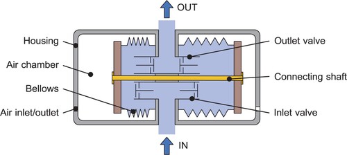
Figure 1 shows the structure of a PDBP. When compressed air is charged into one air chamber, the air in the opposite chamber is exhausted to the atmosphere and the bellows in the charging chamber is compressed, forcing the liquid to get out of the bellows chamber and go into the discharge pipe. As a shaft connects the two bellows rigidly, the compression of one bellows makes the other stretched. With the expansion of the bellows' volume, the pressure in the bellows chamber drops and the liquid is pressed into the chamber. At the end of one stroke, the proximity sensor gives signal to the control unit and the solenoid valve switches, making the compressed air go into the opposite chamber. The continuous reciprocating motion, along with the proper functioning of the internal check valves, makes alternating suction and discharge of the transported liquid into and out of each chamber, resulting in a nearly continuous pumping. Considering the working principle and the symmetric layout, this study only takes single side performances into account.

Figure 1. Sketch of a pneumatic drive bellows pump (PDBP).

                                                

2.1. The test rig

Experiments were carried out in a self-built test rig. Figure 2(a) shows the schematic overview of the experimental system, which is composed of three subsystems, the hydraulic, pneumatic, and measurement system. The hydraulic system, which is the focus of this study, is a closed-loop circulating system containing the test pump. The inlet and outlet pressure of the test pump can be regulated by adjusting the opening of the ball valves cascaded in the system. Pressure sensors and flow meters were set both upstream and downstream of the test pump. To monitor the temperature in the system, a thermal sensor was placed in the water tank. The water tank was specifically designed and has a volume of approximately $34\mathrm{L}$. As shown in Figure 2(a), the end of the outlet pipe was set beneath the free surface of the water tank and baffle-like structures were designed in upper part of the tank, in order to isolate the possible influence of small bubbles generated by high-speed jets from the outlet pipe. In this study, the medium circulating in the hydraulic system was ultra-pure water.

Figure 2. (a) Schematic overview of the experimental system. 1-water tank, 2,8-ball valve, 3,7-flow meter, 4,6-pressure sensor, 5-test pump, 9-thermal sensor, 10-data acquisition card, 11-computer, 12-air source, 13-switch, 14-pressure regulator, 15-solenoid on-off valve, 16-solenoid directional valve, 17,18-silencer, 19,20-quick exhaust valve, 21-cylinder, 22-laser displacement sensor. (b) Photography of the test pump containing a close-up view of the check valve at the bottom left.

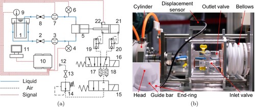
Figure 2(b) illustrates the photography of the test pump. The pump head, which contains the inlet and outlet channel and four check valve cases, was milled out from a cuboid polymethylmethacrylate (PMMA) block. The most significant property of PMMA is its excellent light transmittance, which enables good optical access for the observation of the cavitating flow patterns within the bellows pump. Since this study considers only single side performances, the left 2 valve cases have been closed with end caps. The flexible bellows was actuated by a cylinder through rigid rods. The bore size of the cylinder $D_c$ is $100\mathrm{m}\mathrm{m}$, which is close to the outer diameter of the bellows $D_b$. Table 1 gives the detailed geometrical parameters of the test pump. The stretching and compression amount of the bellows was limited by proximity switches fixed in the cylinder, and the transient displacement was monitored utilizing a laser displacement sensor. A close-up view of the check valve used in the experiment is also shown at the bottom left of Figure 2(b).

Table 1. Geometrical parameters of the test pump.

Parameter	Symbol	Value	Unit
Diameter of inlet (or outlet) pipe (or channel)	d	16.0	$\mathrm{m}\mathrm{m}$
Outer diameter of the bellows	$D_{\mathrm{b}}$	110.5	$\mathrm{m}\mathrm{m}$
Inner diameter of the bellows	$d_{\mathrm{b}}$	76.5	$\mathrm{m}\mathrm{m}$
Effective diameter of the bellows	$d_{\mathrm{b}\mathrm{e}}$	95.0	$\mathrm{m}\mathrm{m}$
Cone angle of check valves	β	60.0	${}^{\circ }$
Outer diameter of check valves	$D_{\mathrm{v}}$	22.5	$\mathrm{m}\mathrm{m}$
Diameter of valve cases	$d_{\mathrm{v}\mathrm{c}}$	24.0	$\mathrm{m}\mathrm{m}$
Axial length of check valves	$L_{\mathrm{v}}$	20.0	$\mathrm{m}\mathrm{m}$
Maximum displacement of check valves	${\chi }_{max}$	9.5	$\mathrm{m}\mathrm{m}$

2.2. Experimental procedure

To remove the gas dissolved in water, the system was operated at relatively high air supply pressure ($p_a\approx 3\mathrm{b}\mathrm{a}\mathrm{r}$), which can make the test pump cavitate intensely, about 8 hours before the experiment. During the experiment, the air supply pressure was fixed at $p_a=1.5\mathrm{b}\mathrm{a}\mathrm{r}$. The experiment started with the inlet and outlet ball valves (2 & 8 in Figure 2(a)) fully open. Tests were conducted at different inlet pressure $p_{\mathrm{i}\mathrm{n}}$. The opening of the inlet ball valve was adjusted to realize the variation of the inlet pressure $p_{\mathrm{i}\mathrm{n}}$, while the outlet ball valve was kept fully open in all cases. For each case, the test pump ran continuously until the integrated flow measured by the flow meter downstream of the test pump (7 in Figure 2(a)) reached the given amount, and the corresponding time consumption was recorded. Table 2 shows the details of all test cases. During the tests, signals from the sensors (pressure, displacement, temperature) were recorded via a National Instrument USB-6216 card. Table 3 lists the key parameters of the sensors used in this study.

Table 2. Details of different test cases.

No.	Inlet pressure $\left(\mathrm{k}\mathrm{P}\mathrm{a}\right)$	Volume $\left(\mathrm{L}\right)$	Time $\left(\mathrm{s}\right)$	Flow rate $\left(\mathrm{L}/\mathrm{m}\mathrm{i}\mathrm{n}\right)$	Temperature ${}^{\circ }\mathrm{C}$
1	91.15	200	857	14.00	11
2	91.13	200	867	13.84	11
3	90.88	200	866	13.86	11
4	90.62	200	878	13.67	11
5	90.32	200	883	13.59	11
6	89.91	200	892	13.45	11
7	89.20	200	909	13.20	11
8	88.41	200	925	12.97	11
9	86.91	200	956	12.55	11
10	85.54	200	988	12.15	11

Table 3. Key parameters of the measuring instruments used in the experiment.

Instrument	Manufacturer and model	Range	Accuracy
Inlet pressure sensor (4 in Figure 2(a))	SEN SCYG314	$-1-1\mathrm{b}\mathrm{a}\mathrm{r}$	$\pm 0.5\mathrm{\%}\mathrm{F}.\mathrm{S}.$
Outlet pressure sensor (6 in Figure 2(a))	SEN SCYG310	$-1-16\mathrm{b}\mathrm{a}\mathrm{r}$	$\pm 0.5\mathrm{\%}\mathrm{F}.\mathrm{S}.$
Outlet flow meter (7 in Figure 2(a))	Keyence FD-Q20C	$0.1-60\mathrm{L}/\mathrm{m}\mathrm{i}\mathrm{n}$	$\pm 0.5\mathrm{\%}\mathrm{F}.\mathrm{S}.$
Thermal sensor (9 in Figure 2(a))	Meacon MIK-WZP	$-50-{200}^{\circ }\mathrm{C}$	$\pm 0.1\mathrm{\%}\mathrm{F}.\mathrm{S}.$
Displacement sensor (22 in Figure 2(a))	Optex CD33-120NV	$120\pm 60\mathrm{m}\mathrm{m}$	$\pm 0.1\mathrm{\%}\mathrm{F}.\mathrm{S}.$

2.3. High-speed visualization

The cavitating flow regimes were captured using high-speed photography. A sketch of this method is shown in Figure 3. During the high-speed measurement, two light sources illuminated the pump head from the front, as illustrated in Figure 3. In this way, the inception, development and collapse process of the vapour cavities can be clearly identified. Since the refractive index of PMMA is relatively close to that of water, the curved inner wall of the circular channel did not present considerable refraction distortion in the high-speed images.

Figure 3. Sketch of the high-speed visualization system.

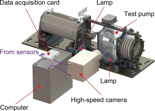
High-speed measurement was carried out utilizing a Phantom v2512 camera equipped with a Laowa $60\mathrm{m}\mathrm{m}f/2.82\times$ Ultra-Macro lens. A small aperture f = 11 was chosen to enlarge the depth of the field. In all cases, an exposure time of $99\mu \mathrm{s}$ was set combined with a frame rate of 10 kHz and a recording time of 1 s. The resolution of each image captured was $1280\times 560\mathrm{p}\mathrm{i}\mathrm{x}\mathrm{e}\mathrm{l}\mathrm{s}$ . The camera was also synchronized with the data acquisition system by the PCC 3.3 software, and the corresponding sensor values at each frame can be recorded.

3. Mathematical models

Today, CFD techniques have become a powerful tool to analyse the detailed spatial and temporal characteristics of the flow fields in reciprocating positive displacement pumps. This section introduces the mathematical models of the numerical simulation describing the unsteady, turbulent, multiphase flow within the bellows pump.

3.1. Governing equations

To accurately simulate the cavitating flow in the bellows pump, a homogeneous mixture model was employed, in which the vapour phase and the liquid phase are treated as interpenetrating continua. Assuming that the fluid is Newtonian and incompressible, with gravity and heat transfer neglected, the Navier–Stokes equations which govern the mass and momentum transport of the homogeneous mixture in Cartesian coordinates are as follows: (1) $\begin{array}{rl}& \frac{\mathrm{\partial }{\rho }_m}{\mathrm{\partial }t}+\frac{\mathrm{\partial }{\rho }_m{u}_j}{\mathrm{\partial }{x}_j}=0\end{array}$(1) (2) $\begin{array}{rl}& \frac{\mathrm{\partial }{\rho }_m{u}_j}{\mathrm{\partial }t}+\frac{\mathrm{\partial }{\rho }_m{u}_i{u}_j}{\mathrm{\partial }{x}_i}=-\frac{\mathrm{\partial }p}{\mathrm{\partial }{x}_j}+\frac{\mathrm{\partial }}{\mathrm{\partial }{x}_i}\left[{\mu }_m(\frac{\mathrm{\partial }{u}_i}{\mathrm{\partial }{x}_j}+\frac{\mathrm{\partial }{u}_j}{\mathrm{\partial }{x}_i})\right]\end{array}$(2) where ${\rho }_m$ is the mixture density, $u_j$ is the velocity of the mixture, p is the pressure, and ${\mu }_m$ is the mixture viscosity. The physical properties of the mixture are defined as the weighed average of the physical properties of each phase. The density and viscosity of the mixture are expressed below: (3) $\begin{array}{rl}& {\rho }_m={\alpha }_l{\rho }_l+{\alpha }_v{\rho }_v\end{array}$(3) (4) $\begin{array}{rl}& {\mu }_m={\alpha }_l{\mu }_l+{\alpha }_v{\mu }_v\end{array}$(4) in which ${\alpha }_l$ is the volume fraction of the liquid, ${\rho }_l$ is the liquid density, ${\mu }_l$ is the liquid dynamic viscosity, ${\alpha }_v$ is the volume fraction of the vapour, ${\rho }_v$ is the vapour density, and ${\mu }_v$ is the vapour dynamic viscosity. The volume fraction of the liquid and the vapour should satisfy the following condition: (5) ${\alpha }_l+{\alpha }_v=1$(5) The mass transfer between the liquid phase and the vapour phase is governed by the following phase transport equation: (6) $\frac{\mathrm{\partial }{\rho }_v{\alpha }_v}{\mathrm{\partial }t}+\frac{\mathrm{\partial }{\rho }_v{\alpha }_v{v}_j}{\mathrm{\partial }{x}_j}={\dot{m}}^{+}-{\dot{m}}^{-}$(6) where $v_j$ is the velocity of the vapour phase, ${\dot{m}}^{+}$ is the evaporation rate, and ${\dot{m}}^{-}$ is the condensation rate.

3.2. Cavitation model

To model the evaporation and condensation process in cavitation, this study adopts the Schnerr–Sauer cavitation model (Schnerr & Sauer, 2001), which is derived on the basis of the Rayleigh-Plesset equation. The Schnerr–Sauer model defines the evaporation rate of water ${\dot{m}}^{+}$ and the condensation rate of vapour ${\dot{m}}^{-}$ as: (7) $\begin{array}{rl}& {\dot{m}}^{+}=C_{eva}\frac{{\rho }_v{\rho }_l}{{\rho }_m}{\alpha }_v(1-{\alpha }_v)\frac{3}{R_{\mathrm{B}}}\sqrt{\frac{2}{3}\frac{p_{\mathrm{t}\mathrm{h}\mathrm{r}}-p}{{\rho }_l}},p<p_{\mathrm{t}\mathrm{h}\mathrm{r}}\end{array}$(7) (8) $\begin{array}{rl}& {\dot{m}}^{-}=C_{con}\frac{{\rho }_v{\rho }_l}{{\rho }_m}{\alpha }_v(1-{\alpha }_v)\frac{3}{R_{\mathrm{B}}}\sqrt{\frac{2}{3}\frac{p-p_{\mathrm{t}\mathrm{h}\mathrm{r}}}{{\rho }_l}},p>p_{\mathrm{t}\mathrm{h}\mathrm{r}}\end{array}$(8) where $C_{eva}$ and $C_{con}$ are the empirical calibration coefficients of evaporation and condensation, and $p_{\mathrm{t}\mathrm{h}\mathrm{r}}$ is the threshold pressure. The bubble radius $R_{\mathrm{B}}$ is defined by: (9) $R_{\mathrm{B}}=\sqrt[3]{\frac{{\alpha }_v}{1-{\alpha }_v}\frac{3}{4\pi n}}$(9) in which n represents the bubble number density. To consider the influence of the turbulent pressure fluctuations, the threshold pressure $p_{\mathrm{t}\mathrm{h}\mathrm{r}}$ is corrected by: (10) $p_{\mathrm{t}\mathrm{h}\mathrm{r}}=p_v+\frac{1}{2}\zeta {\rho }_{l}k$(10) where $p_v$ is the saturated vapour pressure, ζ is the correction coefficient, and k is the turbulent kinetic energy.

In this study, $C_{eva}=1$, $C_{con}=0.2$, $n=1.6\times {10}^{13}$ bubbles/m³ and $\zeta =0.39$ were adopted. The saturated vapour pressure $p_v$ was set to be $1310\mathrm{P}\mathrm{a}$, which was the corresponding value calculated by the Antoine equation at the measured temperature.

3.3. Turbulence model

Turbulence model plays a vital role in CFD simulations for practical engineering problems. Generally, it is unaffordable to solve the Navier–Stokes equations directly in industrial applications, albeit direct numerical simulation (DNS) can give the best temporal and spatial resolution of turbulence. Therefore, to correctly predict turbulence, the governing equations must be averaged or filtered and closed with corresponding turbulence models. Considering feasibility, versatility, and computational efficiency, the Reynolds-averaged Navier–Stokes (RANS) method is adopted in this study.

On the basis of Reynolds decomposition, the governing equations of the homogeneous mixture (Equations (1(1) $\begin{array}{rl}& \frac{\mathrm{\partial }{\rho }_m}{\mathrm{\partial }t}+\frac{\mathrm{\partial }{\rho }_m{u}_j}{\mathrm{\partial }{x}_j}=0\end{array}$(1) ) and (2(2) $\begin{array}{rl}& \frac{\mathrm{\partial }{\rho }_m{u}_j}{\mathrm{\partial }t}+\frac{\mathrm{\partial }{\rho }_m{u}_i{u}_j}{\mathrm{\partial }{x}_i}=-\frac{\mathrm{\partial }p}{\mathrm{\partial }{x}_j}+\frac{\mathrm{\partial }}{\mathrm{\partial }{x}_i}\left[{\mu }_m(\frac{\mathrm{\partial }{u}_i}{\mathrm{\partial }{x}_j}+\frac{\mathrm{\partial }{u}_j}{\mathrm{\partial }{x}_i})\right]\end{array}$(2) )) become: (11) $\begin{array}{rl}& \frac{\mathrm{\partial }{\rho }_m}{\mathrm{\partial }t}+\frac{\mathrm{\partial }{\rho }_m{\overline{u}}_j}{\mathrm{\partial }{x}_j}=0\end{array}$(11) (12) $\begin{array}{rl}& \frac{\mathrm{\partial }{\rho }_m{\overline{u}}_j}{\mathrm{\partial }t}+\frac{\mathrm{\partial }{\rho }_m\overline{u_i{u}_j}}{\mathrm{\partial }{x}_i}\\ & =-\frac{\mathrm{\partial }\overline{p}}{\mathrm{\partial }{x}_j}+\frac{\mathrm{\partial }}{\mathrm{\partial }{x}_i}[{\mu }_m(\frac{\mathrm{\partial }{\overline{u}}_i}{\mathrm{\partial }{x}_j}+\frac{\mathrm{\partial }{\overline{u}}_j}{\mathrm{\partial }{x}_i})-{\rho }_m\overline{u_i^{\mathrm{\prime }}{u}_j^{\mathrm{\prime }}}]\end{array}$(12) Compared with Equations (1(1) $\begin{array}{rl}& \frac{\mathrm{\partial }{\rho }_m}{\mathrm{\partial }t}+\frac{\mathrm{\partial }{\rho }_m{u}_j}{\mathrm{\partial }{x}_j}=0\end{array}$(1) ) and (2(2) $\begin{array}{rl}& \frac{\mathrm{\partial }{\rho }_m{u}_j}{\mathrm{\partial }t}+\frac{\mathrm{\partial }{\rho }_m{u}_i{u}_j}{\mathrm{\partial }{x}_i}=-\frac{\mathrm{\partial }p}{\mathrm{\partial }{x}_j}+\frac{\mathrm{\partial }}{\mathrm{\partial }{x}_i}\left[{\mu }_m(\frac{\mathrm{\partial }{u}_i}{\mathrm{\partial }{x}_j}+\frac{\mathrm{\partial }{u}_j}{\mathrm{\partial }{x}_i})\right]\end{array}$(2) ), additional terms appear in the momentum equation  (12(12) $\begin{array}{rl}& \frac{\mathrm{\partial }{\rho }_m{\overline{u}}_j}{\mathrm{\partial }t}+\frac{\mathrm{\partial }{\rho }_m\overline{u_i{u}_j}}{\mathrm{\partial }{x}_i}\\ & =-\frac{\mathrm{\partial }\overline{p}}{\mathrm{\partial }{x}_j}+\frac{\mathrm{\partial }}{\mathrm{\partial }{x}_i}[{\mu }_m(\frac{\mathrm{\partial }{\overline{u}}_i}{\mathrm{\partial }{x}_j}+\frac{\mathrm{\partial }{\overline{u}}_j}{\mathrm{\partial }{x}_i})-{\rho }_m\overline{u_i^{\mathrm{\prime }}{u}_j^{\mathrm{\prime }}}]\end{array}$(12) ). The term $-{\rho }_m\overline{u_i^{\mathrm{\prime }}{u}_j^{\mathrm{\prime }}}$, which represents the effect of turbulence, is called Reynolds stresses. In order to close Equations (11(11) $\begin{array}{rl}& \frac{\mathrm{\partial }{\rho }_m}{\mathrm{\partial }t}+\frac{\mathrm{\partial }{\rho }_m{\overline{u}}_j}{\mathrm{\partial }{x}_j}=0\end{array}$(11) ) and (12(12) $\begin{array}{rl}& \frac{\mathrm{\partial }{\rho }_m{\overline{u}}_j}{\mathrm{\partial }t}+\frac{\mathrm{\partial }{\rho }_m\overline{u_i{u}_j}}{\mathrm{\partial }{x}_i}\\ & =-\frac{\mathrm{\partial }\overline{p}}{\mathrm{\partial }{x}_j}+\frac{\mathrm{\partial }}{\mathrm{\partial }{x}_i}[{\mu }_m(\frac{\mathrm{\partial }{\overline{u}}_i}{\mathrm{\partial }{x}_j}+\frac{\mathrm{\partial }{\overline{u}}_j}{\mathrm{\partial }{x}_i})-{\rho }_m\overline{u_i^{\mathrm{\prime }}{u}_j^{\mathrm{\prime }}}]\end{array}$(12) ), the Reynolds stresses must be modelled. The Boussinesq hypothesis relates the Reynolds stresses linearly to the averaged strain rate: (13) $R_{ij}=-{\rho }_m\overline{u_i^{\mathrm{\prime }}{u}_j^{\mathrm{\prime }}}={\mu }_t(\frac{\mathrm{\partial }{\overline{u}}_i}{\mathrm{\partial }{x}_j}+\frac{\mathrm{\partial }{\overline{u}}_j}{\mathrm{\partial }{x}_i})-\frac{2}{3}{\rho }_{m}k{\delta }_{ij}$(13) where ${\mu }_t$ is the turbulent viscosity (also called the eddy viscosity), $k=\frac{1}{2}\overline{u_j^{\mathrm{\prime }}{u}_j^{\mathrm{\prime }}}$ is the turbulent kinetic energy, and ${\delta }_{ij}$ is the Kronecker delta. Depending on the methods used to compute the turbulent viscosity ${\mu }_t$, the linear eddy viscosity model can be divided into several categories.

Numerous existing studies have utilized linear eddy viscosity models, such as Spalart & Allmaras model (Al-Azawy et al., 2016; Pan et al., 2019), $k-ϵ$ model (Alberto et al., 2019; S. Wu & Wei, 2019), and $k-\omega$ model (Li & Yu, 2021; Obidowski et al., 2018), to simulate the turbulent flow field within reciprocating positive displacement pumps with reasonable accuracy. In this study, the Shear-Stress Transport (SST) $k-\omega$ model was used, as it is better at predicting adverse pressure gradients and flow separation. With the SST $k-\omega$ model, the turbulent viscosity ${\mu }_t$ can be computed as a function of the turbulent kinetic energy k and the specific dissipation rate ω: (14) ${\mu }_t=\frac{{\rho }_{m}k}{\omega }{[max(\frac{1}{{\alpha }^{\ast }},\frac{S{F}_2}{a_1\omega })]}^{-1}$(14) where ${\alpha }^{\ast }$ is the low-Reynolds number correction coefficient, S is the strain rate magnitude, $F_2$ is a blending function, $a_1$ is a model constant whose value is 0.31. More details of the SST $k-\omega$ turbulence model can be found in Menter's work (Menter, 1994).

4. Numerical setup

The commercial package ANSYS${}^{\circledR }$ FLUENT 2020 R2 was employed to solve the set of partial differential equations describing the turbulent, cavitating flow using the finite volume method. This section presents the detailed setup of the numerical model, including a description of the physical problem to be modelled, the discretization method of the continuous geometric model, the strategy for updating the deformed volume mesh, the simplified 6-DOF model of the check valves and some crucial settings of the solver.

4.1. Problem description

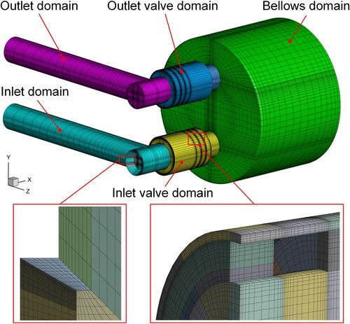
The turbulent, cavitating flow in a domain whose critical features are the same as the test pump was simulated in this study. The computational domain, which is illustrated in Figure 4, is composed of the inlet pipe, inlet channel, inlet valve, bellows, outlet valve, outlet channel, and outlet pipe. In Figure 4, an inlet pipe with a length of 7.5d is connected to the inlet channel to make the entering flow as smooth as possible. The bellows, which is flexible and only compressed or stretched axially, is simplified as an equivalent cylinder with effective diameter $d_{be}$. The corresponding geometrical data of the computational domain can be found in Table 1.

Figure 4. Schematic of the computational domain.

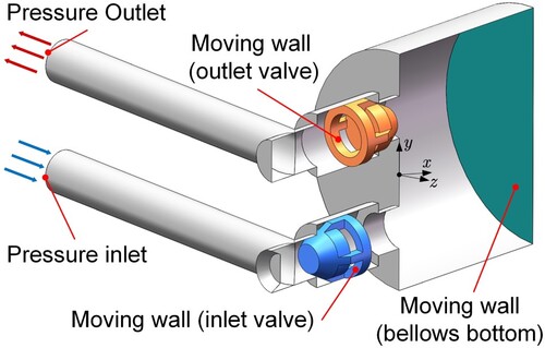
The boundary conditions imposed on the computational model are also presented in Figure 4. The inlet and outlet of the computational domain were defined as pressure inlet and pressure outlet respectively, whose values are kept the same as the experimental measurement. All 10 groups of data listed in Table 2 were adopted to simulate the flow regimes within the test pump at different inlet pressure $p_{\mathrm{i}\mathrm{n}}$. The inlet valve, outlet valve, and bellows bottom were set as no-slip wall whose positions are updated dynamically during the simulation. The detailed configuration of the moving boundaries can be found in Section 4.3. All other solid boundaries were defined as no-slip wall.

4.2. Grid generation

Considering efficiency and accuracy of the calculation, structured mesh techniques were adopted in this study. The structured mesh was generated by the ANSYS${}^{\circledR }$ Meshing module with the geometric model pre-subdivided into small bodies whose faces can generate a mapped mesh. A baseline coarse mesh was first generated, based on which precursor steady-state simulation was conducted to identify critical regions and estimate required grid scales by integral length scale. Figure 5 presents the structured mesh used for the simulation. Local refinements have been conducted in the near-wall region, small gaps, and the region around the end-ring of the check valves.

Figure 5. Structured mesh used for the simulation. Different domains are illustrated with different colours. Enlarged views show local refinements in the near-wall region and the region around the end-ring of the inlet valve.

To evaluate the spatial discretization error in numerical simulations, this study adopted the most popular grid convergence index (GCI) method (Kim et al., 2019; Lin et al., 2023; Trivedi et al., 2013). Three groups of mesh, which are composed of 237,408 (coarse), 561,736 (medium), and 1,259,640 (fine) elements, were used to verify grid independence. On the basis of the three groups of mesh, simulations were conducted for Case 1 in Table 2. The time-averaged flow rate $\overline{Q}$ is used for grid convergence analysis, and the results are listed in Table 4. The detailed procedure of the GCI method and the meaning of the parameters listed in Table 4 can be found in Celik et al. (2008). The GCI values are all within 2%, indicating that the solutions of the grids are in the range of asymptotic convergence (Hui et al., 2023; Kan et al., 2023). Table 5 gives the approximate computational time, and relative error ε of the predicted time-averaged flow rate $\overline{Q}$ with the experimental value, of the three groups of mesh. For each case, two high-performance compute nodes were employed, and each node is with two 12-core Intel(R) Xeon(R) Silver 4214R CPU @ 2.40 GHz and 256 GiB RAM. The computational cost grows significantly with the grid number. The relative error ε decreases with the increase of the gird number, but all three groups of mesh can predict the time-averaged flow rate $\overline{Q}$ with reasonable accuracy. Thus, considering computational accuracy and efficiency, the mesh with the medium number of elements was selected for this study. Figure 6 shows the distribution of time-averaged $y^{+}$ during the suction stroke. The maximum value is kept within $y^{+}<100$, which meets the requirement of $y^{+}$-insensitive wall treatment utilized for the $\mathrm{S}\mathrm{S}\mathrm{T}k-\omega$ model in FLUENT (Ansys, 2020).

Figure 6. Distribution of time-averaged $y^{+}$ during the suction stroke (Case 1).

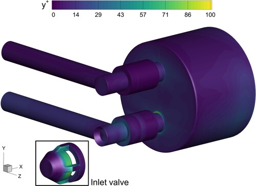
Table 4. Estimations of discretization error.

Parameter	$\varphi =\overline{Q}$
$N_1$,$N_2$,$N_3$	1,259,640, 561,736, 237,408
$r_{21}$,$r_{32}$	1.31, 1.33
${\varphi }_1$,${\varphi }_2$,${\varphi }_3$	13.55, 13.47, 13.35
p	1.63
${\varphi }_{ext}^{21}$,${\varphi }_{ext}^{32}$	13.68, 13.67
$e_a^{21}$,$e_a^{32}$	0.55%, 0.93%
$e_{ext}^{21}$,$e_{ext}^{32}$	0.99%, 1.4%
$GC{I}_{21}$,$GC{I}_{32}$	1.25%, 1.95%

Table 5. Information of meshes used for grid independence analysis.

Mesh	Number of elements	Approx. computational time ($\mathrm{h}$)	ε
Coarse	237,408	37	4.65%
Medium	561,736	56	3.76%
Fine	1,259,640	84	3.22%

4.3. 6-DOF model and dynamic mesh strategy

During the working process of PDBPs, positions of several boundaries are changing: bellows bottoms reciprocate to generate periodic changes of the bellows volume, check valves open and close alternatively to make unidirectional flow into or out of the bellows chamber. The motion of the bellows bottoms is driven by external input power, whereas the operation of the check valves is owing to a combination of fluid forces and spring forces. Therefore, in modelling PDBPs, dynamic response of check valves to hydrodynamic and other external loads, as well as dynamic update of corresponding volume mesh in deforming regions, has to be considered.

The check valves are treated as rigid bodies whose motion is simplified as one degree of freedom translation and determined by Newton's second law. The forces acting on the inlet check valve are illustrated in Figure 7, including the pressure force $F_p$, the drag force $F_r$ and the spring force $F_s$. As the motion of the check valve is horizontal, gravity is not considered here. The governing equation for the translation motion of the check valve gives: (15) $m_{\mathrm{v}}{a}_x=F_p-F_r-F_s$(15) where $m_{\mathrm{v}}$ is the mass of the check valve, $a_x$ is the x-component of acceleration of the check valve. The pressure force $F_p$ and the drag force $F_r$ are calculated by surface integral of the pressure and the shear stress acting on the check valve. The spring force $F_{\mathrm{s}}$ is determined by the Hooke's law according to the displacement of the check valve and the given stiffness coefficient. At each time step, Equation (15(15) $m_{\mathrm{v}}{a}_x=F_p-F_r-F_s$(15) ) is solved, and the position of the check valve is updated accordingly by numerical integration. The mass of the check valve $m_{\mathrm{v}}$, the moving direction, the stiffness coefficient and preload of the spring, and the maximum opening positions in the numerical model are kept the same as the test pump. As the geometric topology of the computational domain has to be kept consistent throughout the whole simulation, a small clearance is maintained in the fully closing position of the valve, and in this study, it has been fixed to $\chi =0.16\mathrm{m}\mathrm{m}$. For the axially moving bellows bottom, the position of its gravity center is specified by corresponding displacement profiles measured experimentally by the laser displacement sensor.

Figure 7. Schematic of the forces acting on the inlet check valve at the opening process and details of layering technique for mesh reconstruction.

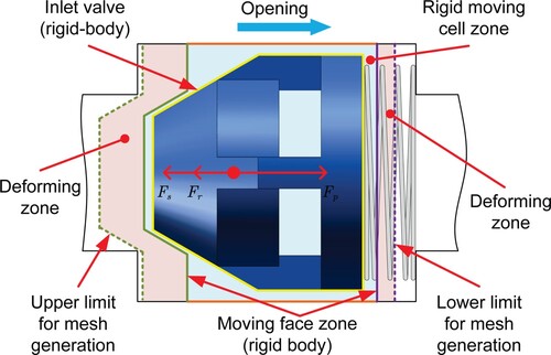
Considering feasibility, efficiency, and computational economy, this study adopts the layering method to update the volume mesh in the deforming regions subject to the translation of the bellows bottom and the check valves. Figure 7 shows the details of the layering technique of the inlet valve. The inlet valve is set as a rigid body whose motion is predicted by the 6-DOF model. To keep the boundary layer meshes around the valve undeformed throughout the whole simulation, the near valve region encapsulated with structured mesh is also treated as a rigid body moving with the valve passively. The layers of cells upstream and downstream of the moving face zone can be split or merged with the movement of the inlet valve. The dynamic update of the mesh around the outlet valve is set similarly.

4.4. Solver settings

In this study, the governing equations of fluid flow and rigid-body motion were solved separately, which is the so-called partitioned CFD/6-DOF solver. The partitioned CFD/6-DOF solver has been widely used in modelling reciprocating pumps (Alberto et al., 2019; Iannetti et al., 2015). When utilizing the partitioned CFD/6-DOF solver, special care has to be taken in choosing whether the explicit (loosely coupled) or the implicit (tightly coupled) approach. The explicit approach is cost-efficient with the dynamic mesh updating at the beginning of each time step, whereas it can be unstable in some specific occasions. The instability of the explicit approach can be handled with the implicit approach (Campbell, 2010), in which mesh updates iteratively within the time steps. Two parameters were found critical to the numerical stability of the partitioned CFD/6-DOF solver: density ratio and time step size (Dunbar et al., 2015). In this study, the density ratio of the fluid (the medium used in the simulation is water, ${\rho }_f=998{\mathrm{k}\mathrm{g}/\mathrm{m}}^3$) with respect to the solid (the check valves are made of PTFE, ${\rho }_s=2320{\mathrm{k}\mathrm{g}/\mathrm{m}}^3$) is much smaller than unity, which reduces the risk of numerical instability. After several trials and validations, the explicit partitioned CFD/6-DOF solver (Algorithm 4.1) was adopted. The time step size was chosen to be $2.5\times {10}^{-5}\mathrm{s}$, which was a balance between stability and economy. For each case, the duration of the simulation was $0.625\mathrm{s}$, which started with the delivery stroke and contained one and a half cycles. Table 6 gives a summary of the settings of the fluid solver.

Table 6. Summary of the settings of the fluid solver.

Settings	Details
Pressure-velocity coupling	PISO
Turbulence model	SST $k-\omega$
Multiphase model	Mixture
Cavitation model	Schnerr–Sauer
Spatial discretization	Pressure	PRESTO!
	Momentum	Second-order upwind
	Turbulent kinetic energy	First-order upwind
	Turbulent dissipation rate	First-order upwind
	Volume fraction	First-order upwind
Transient formulation	First-order implicit
Under-relaxation factors	Pressure	0.3
	Momentum	0.7
	Turbulent kinetic energy	0.8
	Turbulent dissipation rate	0.8
	Volume fraction	0.5
Residuals	Continuity	${10}^{-3}$
	X-velocity	${10}^{-5}$
	Y-velocity	${10}^{-5}$
	Z-velocity	${10}^{-5}$
	Turbulent kinetic energy	${10}^{-5}$
	Turbulent dissipation rate	${10}^{-5}$
	Volume fraction	${10}^{-5}$
Time step size $\left(\mathrm{s}\right)$	$2.5\times {10}^{-5}$
Max iteration per time step	50

5. Results and discussion

5.1. Comparison of performance characteristics

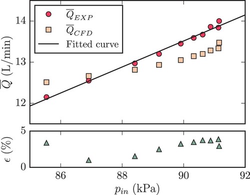
To verify the reliability of the numerical model, the performance characteristics predicted by the CFD model are compared with the experimental data in this section. Figure 8 compares the time-averaged flow rate $\overline{Q}$ calculated by the unsteady numerical model established in Section 3 and that obtained from experimental measurement as a function of inlet pressure $p_{\mathrm{i}\mathrm{n}}$. During the experiment, the time consumption of the test pump to transfer $200\mathrm{L}$ water was recorded, based on which the time-averaged flow rate was calculated and shown in Table 2. For the numerical model, the flow rate was estimated by dividing the output flow rate in a single cycle with the period. It can be seen from the numerical results in Figure 8 that the time-averaged flow rate $\overline{Q}$ drops with the decrease of the inlet pressure $p_{\mathrm{i}\mathrm{n}}$, which agrees well with the experimental results. Figure 8 also illustrates the error ϵ between the numerical results and the fitted values of the experimental results, and the maximum value is kept within $5\mathrm{\%}$. Therefore, it can be concluded that the numerical model can predict the flow rate in cavitation conditions with reasonable accuracy. The discrepancy between the experimental and numerical results exists, on account of the limitation of the cavitation model and the turbulence model. In this study, the cavitation model adopts the homogeneous mixture assumption, in which the vapour phase and the liquid phase share the same velocity field and pressure field, and it does not take the effect of non-condensable gases and surface tension into account. Although the turbulent kinetic energy is specifically introduced in the cavitation model in Section 3.2, the interaction between cavitation and turbulence is rather complex. Moreover, the RANS modelling of turbulence can result in the overestimation of the eddy viscosity in cavitation areas (Chebli et al., 2021).

Figure 8. Comparison of time-averaged flow rate $\overline{Q}$ computed by numerical model and that obtained from experimental measurement at different inlet pressure $p_{\mathrm{i}\mathrm{n}}$. The bottom figure shows the error ϵ between the numerical results and the fitted values of the experimental results.

5.2. Transient cavitating flow patterns

Cavitation bubbles were captured by high-speed camera during the suction stroke in all test cases. Figure 9 shows typical captures of the vapour structures in PDBPs. Cavitation was observed to incept at three different locations with varying spatial and temporal characteristics in the suction passage. In Figure 9(a), cavities initiate at the corner (intersection of the inlet pipe and the inlet channel) with the opening of the inlet valve. The cavities at the corner appear as a sheet-like structure attaching to the inner wall of the corner and with small bubbles shedding from the trailing edge. Shortly after inception, the small sheet-like structure breaks up into several tiny filaments and flows downstream. Figure 9(b) illustrates the ribbon-like and highly rotational vapour structure at the core of the inlet channel, which incepts after the opening process of the inlet valve. In Figure 9(b), only one ribbon-like structure is shown at the lower part of the inlet channel; however, similar structures can also appear at the upper part in some cases. The surface of the ribbon-like cavities is wavy, indicating the instability of these structures. The stretching, breaking up, and shedding of these structures are also shown in Figure 9(b). The occurrence of the aforementioned two types of cavitation is almost transient, In comparison, the vapour structures at the bottom of the inlet valve (Figure 9(c)) can exist in nearly $70\mathrm{\%}$ of the suction stroke. When the inlet valve is fully opened, vapour structures are observed shedding from the inner part of the end-ring near the front guide bars (indicated by red rectangles in Figure 9(c)). The shed small cavities flow with the stream and expand as unstable vortical structures at the core of the end-ring. Clusters of rotational vapour structures are also observed downstream of the inlet valve.

Figure 9. High-speed captures of typical vapour structures in PDBPs (Case 1). (a) Sheet-like cavities at the corner (intersection of the inlet pipe and the inlet channel). (b) Ribbon-like cavities at the core of the inlet channel. (c) Cavitation at the bottom of the inlet valve.

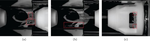
As for the three types of cavitation mentioned above, the cavitation bubbles generated at the bottom of the inlet valve play a vital role in the suction process at varying operating conditions and can severely influence the proper functioning of the pump. The intensity of the cavitation at the bottom of the inlet valve can be relatively high for a long duration, which can narrow the effective flow area and decrease the suction efficiency. Besides, when the broken-up cavities generated at the bottom of the inlet valve flow downstream into the bellows chamber, which is the generator of low pressure, they can expand abruptly and decrease the effective suction volume. Furthermore, cavitation with high intensity and long duration can affect specific chemical or physical properties of the transported media, which are sensitive to mechanical handling. Figure 10 illustrates the initiation and development process of cavitation predicted by the numerical model at the bottom of the inlet valve when it is fully opened. The vapour structures are predicted by iso-surfaces of vapour volume fraction ${\alpha }_v=0.01$ (blue in Figure 10). Iso-surfaces of ${\alpha }_v=0.5$ (red in Figure 10) are also illustrated to indicate regions of high cavitation intensity. From Figure 10(a), the trailing edge of the valve head, both the leading edge and the trailing edge of the end-ring are prone to initiate cavitation. However, based on the predicted results, the cavities at the trailing edge of the valve head and the end-ring only sustain for extremely short duration and no further development can be observed. Dominant cavitation region concentrates at the inner leading edge of the end-ring, with higher intensity, longer duration, and more complex morphology evolution. Initially, the cavitation bubbles appear as slender structures in the dominant cavitation region (Figure 10(a)). For the suction flow has experienced a ${90}^{\circ }$ sharp turning not far from the inlet valve case, the flow past the inlet valve is subsequently non-uniform and with higher speed at the region with positive z coordinates, where the sizes of the inception vapour structures are generally larger and the intensities are also higher. As shown in Figure 10(b), at the inner leading edge of the end-ring, the cavities with positive z coordinates grow in streamwise direction with higher speed at the middle and lower speed at the ends; however, the cavities with negative z coordinates quickly start to shrink. Due to the existence of the velocity gradient of flow past the leading edge of the end-ring in the circumferential direction, the large-scale cavities with positive z coordinates break up into small end parts and large middle parts (Figures 10(d–e)), which then shed downstream (Figure 10(f)) and collapse. Finally, the small end parts near the guide bars increase in size and become dominant (Figure 10(f)), which also corresponds with the high-speed observation.

Figure 10. Initiation and development process of vapour structures (iso-surfaces of ${\alpha }_v=0.01$ coloured by blue, ${\alpha }_v=0.5$ coloured by red) at the bottom of the inlet valve when it is fully opened (Case 1). $T_0$ is the instant when cavitation incepts at the bottom of the inlet valve. (a) $T_0$. (b) $T_0+0.2\mathrm{m}\mathrm{s}$. (c) $T_0+0.4\mathrm{m}\mathrm{s}$. (d) $T_0+0.6\mathrm{m}\mathrm{s}$. (e) $T_0+0.8\mathrm{m}\mathrm{s}$ and (f) $T_0+1.0\mathrm{m}\mathrm{s}$.

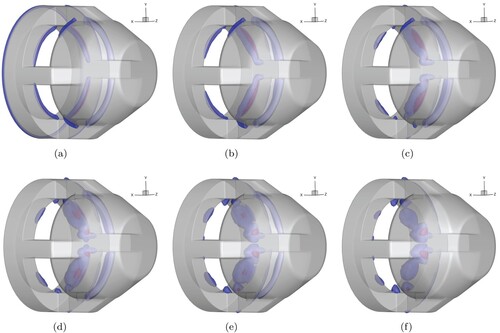
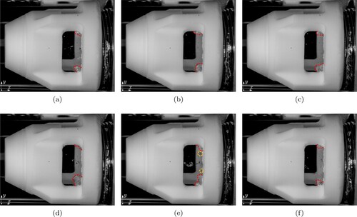
Figure 11 illustrates the high-speed captures of the typical evolution process of vapour structures at the bottom of the inlet valve. As the ring-like structure at the bottom of the valve limits the optical access of the flow details within the end-ring, the high-speed camera can only capture limited parts of the flow field. Large-scale vapour structures exist near the guide bar at the inner part of the end-ring, which are outlined by red dashed curves in Figure 11, and are unstable with the growth, break up, and shedding. The shed vapour filaments are indicated by orange dashed circles in Figure 11(e). Moreover, in Figure 11, visible cavities appear mainly in positive z regions, which agrees well with the numerical prediction.

Figure 11. Typical evolution process of vapour structures at the bottom of the inlet valve captured by high-speed camera (Case 1). The vapour structures near the guide bar at the inner part of the end-ring are outlined by red dashed curves. The shed vapour filaments are indicated by orange dashed circles. The time interval between the two frames is $0.5\mathrm{m}\mathrm{s}$.

5.3. Shear in PDBPs

Generally, no special care should be taken of shear when designing or maintaining hydraulic machinery. However, when handling with specific shear-sensitive medium, excessive exposure to shear can result in severe consequences, such as hemolysis in blood pumps (Y. Liu et al., 2022) and agglomeration in CMP slurry pumps (Seo et al., 2014). Through exposing CMP slurries to different quantified shear rates for various durations using rheometer, it was found that when subjected to moderate shear rates ($100{\mathrm{s}}^{-1}-1000{\mathrm{s}}^{-1}$), not only agglomeration will not happen for sufficient long exposure, but the initially weakly held agglomerates can also be broken down; however, once the shear rates reach certain level (generally $>2000{\mathrm{s}}^{-1}$), even short exposure can result in agglomeration (Khanna et al., 2018). Therefore, the Camp number, which is defined as shear rate times exposure time, was proposed by Khanna, Gupta, et al. (2019) to represent the total shear, and the threshold value to cause agglomeration is among ${10}^5\sim {10}^6$ for different pH conditions. In CMP slurry distribution systems, the slurries in the tank are circulated continuously by PDBPs to mix all ingredients thoroughly and keep uniformity of physical properties. Although the exposure time of the slurries to high shear may not be that high in one single cycle, the hurt induced by shear can be accumulated, and agglomeration occurs in the end. Thus, understanding the shear in PDBPs quantitatively is vitally important.

Figure 12 compares the time series of volume-averaged shear rate $\mathcal{S}$ in different parts of PDBPs during the suction stroke. The shear rate $S=\sqrt{2S_{ij}{S}_{ij}}$ is defined as the norm of the strain rate tensor $S_{ij}$. Initially, the volume-averaged shear rate $\mathcal{S}$ is sufficiently low in all domains. With the opening of the inlet valve, the shear level in different parts of PDBPs increases more or less. Within the suction stroke, the shear exposed to the medium in the inlet domain and bellows domain is acceptable. Nevertheless, the volume-averaged shear rate $\mathcal{S}$ in the inlet valve domain approaches $3000{\mathrm{s}}^{-1}$ for a sufficiently long duration.

Figure 12. Time series of volume-averaged shear rate $\mathcal{S}$ in different parts of PDBPs from the beginning of the suction stroke (Case 1).

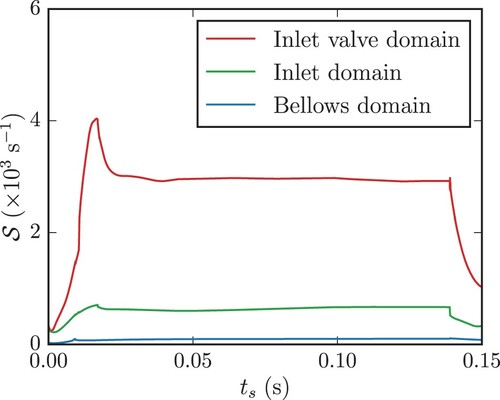
Figure 13. Histograms of time-averaged shear rate $\overline{S}$ in the inlet valve case during the suction stroke (Case 1).

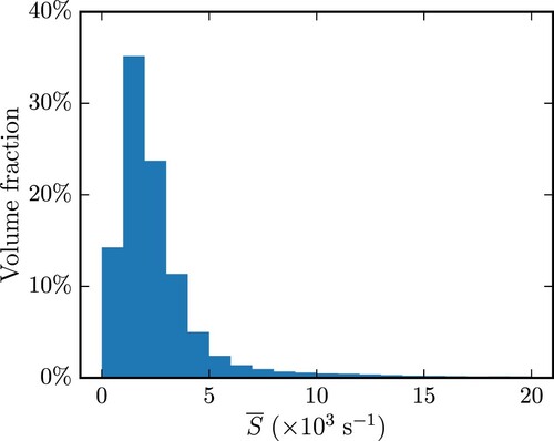
Figure 13 shows the histograms of time-averaged shear rate $\overline{S}$ in the inlet valve during the suction stroke. The vertical axis in Figure 13 indicates the volume fraction of the volume of cells with corresponding properties with respect to the total volume of the inlet valve case. It is apparent from Figure 13 that only about $15\mathrm{\%}$ volume of the inlet valve case is exposed to shear rate $\overline{S}<1\times {10}^3{\mathrm{s}}^{-1}$, which is the aforementioned moderate shear rate. Besides, the accumulated volume of high shear rate $\overline{S}>2\times {10}^3{\mathrm{s}}^{-1}$ occupies almost $50\mathrm{\%}$ of the inlet valve case, and certain volumes are even exposed to extremely high shear. That is to say, it is highly possible for the shear-induced agglomeration to occur in the inlet valve.

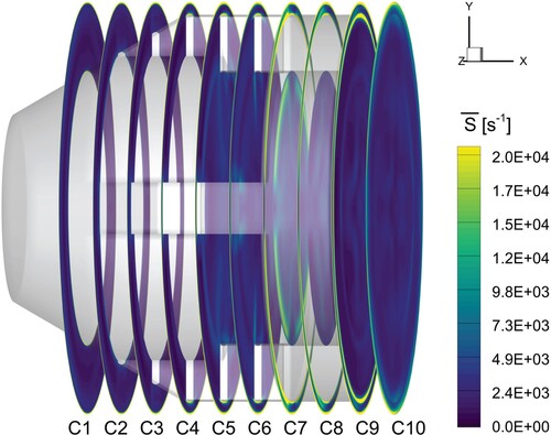
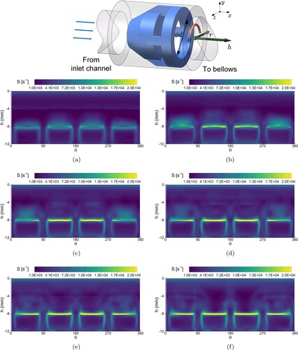
The detailed distribution of the time-averaged shear rate $\overline{S}$ at different axial slices of the inlet valve can be seen in Figure 14. It is apparent that the shear rate $\overline{S}$ is much lower at the slices of the valve head (C1–C3). Owing to the contraction effect, high shear region starts to appear at the ring-slit between the outer surface of the guide bar and the valve case (C4). The separated flow downstream of the valve head can also raise the local shear level (C5–C6). The high shear regions concentrate at the bottom of the valve, especially in the vicinity of the leading edge of the end-ring (C7). As illustrated in Section 5.2, cavitation also initiate at the leading edge of the end-ring, indicating that shear may interact with cavitation. Thus, the next section will give a thorough analysis of the relationship between shear and cavitation.

Figure 14. Contour of time-averaged shear rate $\overline{S}$ at different slices of the inlet valve during the suction stroke (Case 1).

5.4. Relationship between cavitation and shear

This section investigates the relationship between cavitation and shear at the bottom of the inlet valve on the basis of vortex analysis. The flow past the inlet valve can be simplified as confined flow past a bluff body (short chamfered cylinder), in the near wake of which a circular ring with rectangular cross-section is placed. Previous studies revealed that the wake of the bluff bodies can be of large size, in which complicated turbulent structures exist (Derakhshandeh & Alam, 2019). In this study, the existence of the end-ring in the wake of the valve head can even complicate the turbulent flow structures at the bottom of the valve. Vortical structures are a representative component of turbulence and can be found in many typical flows, such as cavitating flow (Arndt, 2002) and shear flow (X. Wu, 2019). To identify the three-dimensional vortical structures around the inlet valve, the new omega vortex identification method (C. Liu et al., 2016) is adopted in this paper. Based on the idea of separating the vortical part from the whole vorticity, a parameter Ω is defined as: (16) $\begin{array}{rl}\mathrm{\Omega }& =\frac{b}{a+b+\xi }\\ a& =trace\left({\mathit{A}}^T\mathit{A}\right)\\ b& =trace\left({\mathit{B}}^T\mathit{B}\right)\end{array}$(16) where $\mathit{A}$ and $\mathit{B}$ are respectively the symmetric and anti-symmetric part of the velocity gradient tensor, and ξ is a small positive number used to avoid division by zero. Different from the Q and ${\lambda }_2$ methods which require proper selection of a widely changed threshold from case to case, fixed value $\mathrm{\Omega }=0.52$ recommended by C. Liu et al. (2016) can capture both the strong and weak vortices properly.

Figure 15 shows the evolution process of the vortical structures around the inlet valve at its fully open position from the instant of cavitation inception at the leading edge of the end-ring. The utilization of the RANS model limits the capture of the small vortices. As a result of the non-uniform incoming flow, the volume of the vortical structures is generally larger at the region with positive z coordinates. In Figure 15(a), most visible vortical structures are circumferential. However, with the evolution of the flow field, these structures are stretched, dilated, or distorted, and the three-dimensionality of the flow increases. Large pockets of separation vortices can be found at the trailing edge of the valve head, as well as at the leading edges of the end-ring. Compared with the incipient vapour structures shown in Figure 10, it is observed that the formation and development process of the dominant vapour structures both take place within the separation vortices at the leading edge of the end-ring. Figure 16 presents the distribution of shear rate S at different instants corresponding to each figure in Figure 15 at the cylindrical slice of the inlet valve, which is very close to the inner surface of the end-ring. A cylindrical coordinate system is established and utilized in Figure 16 to facilitate the analysis. The dashed line in Figure 16 indicates the position of the leading edge of the end-ring. As can be seen from Figure 16(a), locally high shear rate S appears at the leading edge of the end-ring, and there is no significant difference between the four edges at $T_0$. Owing to the non-uniformity of the incoming flow, the shear rate S grows much faster in positive z regions, and the values are also much larger. Comparing Figure 15 with Figure 16, it can be seen that vortical structures exist at the region of high shear, and higher value of shear rate S generally corresponds to larger vortical structures. As regions of high shear are usually with large velocity gradient, vortices are prone to appear in these regions.

Figure 15. Evolution process of vortical structures (iso-surfaces of $\mathrm{\Omega }=0.52$ coloured by green) at the bottom of the inlet valve when it is fully opened (Case 1). $T_0$ is the instant when cavitation incepts at the leading edge of the end-ring. (a) $T_0$. (b) $T_0+0.2\mathrm{m}\mathrm{s}$. (c) $T_0+0.4\mathrm{m}\mathrm{s}$. (d) $T_0+0.6\mathrm{m}\mathrm{s}$. (e) $T_0+0.8\mathrm{m}\mathrm{s}$ and (f) $T_0+1.0\mathrm{m}\mathrm{s}$.

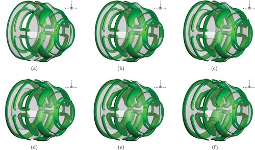
Figure 16. Evolution of the distribution of shear rate S at a cylindrical slice of the inlet valve case, which cuts through the cavities and the vortices at $r\approx 0.47d$ (Case 1). $T_0$ is the instant when cavitation incepts at the leading edge of the end-ring. A cylindrical coordinate system is established to facilitate the analysis. (a) $T_0$. (b) $T_0+0.2\mathrm{m}\mathrm{s}$. (c) $T_0+0.4\mathrm{m}\mathrm{s}$. (d) $T_0+0.6\mathrm{m}\mathrm{s}$. (e) $T_0+0.8\mathrm{m}\mathrm{s}$ and (f) $T_0+1.0\mathrm{m}\mathrm{s}$.

For incompressible fluids, the pressure field can be related with the velocity field by the Poisson equation: (17) $-\frac{1}{\rho }\frac{{\mathrm{\partial }}^{2}p}{\mathrm{\partial }{x}_i^2}=\frac{\mathrm{\partial }{w}_i}{\mathrm{\partial }{x}_j}\frac{\mathrm{\partial }{w}_j}{\mathrm{\partial }{x}_i}$(17) Through simple manipulation, the Poisson equation becomes: (18) $-\frac{1}{\rho }\frac{{\mathrm{\partial }}^{2}p}{\mathrm{\partial }{x}_i^2}=(S_{ij}+{\mathrm{\Re }}_{ij})(S_{ij}-{\mathrm{\Re }}_{ij})=S_{ij}{S}_{ij}-\frac{1}{2}{\omega }_i^2$(18) where $w_i$ is the velocity tensor, $S_{ij}$ is the strain rate tensor, ${\mathrm{\Re }}_{ij}$ is the rotation tensor, and ${\omega }_i$ is the vorticity vector. Equation (18(18) $-\frac{1}{\rho }\frac{{\mathrm{\partial }}^{2}p}{\mathrm{\partial }{x}_i^2}=(S_{ij}+{\mathrm{\Re }}_{ij})(S_{ij}-{\mathrm{\Re }}_{ij})=S_{ij}{S}_{ij}-\frac{1}{2}{\omega }_i^2$(18) ) indicates that the coherent structures where vorticity concentrates can give rise to regions of locally low pressure in which cavitation bubbles are prone to initiate. Figure 17 presents the distribution of the circumferential vorticity ${\omega }_{\theta }$, which is the dominant component of the vorticity vector at the leading edge of the end-ring, at different instants corresponding to each figure in Figure 15 at cylindrical slice of the inlet valve. 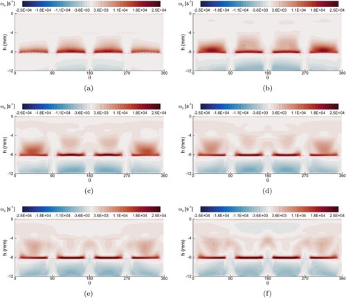Large values of circumferential vorticity ${\omega }_{\theta }$ concentrate at the leading edge of the end-ring, especially at the region with positive z coordinates, which coincides with the cavitation region and the high shear region. Therefore, it could be concluded that the high-intensity vortices generated owing to strong shear result in the inception of cavitation at the leading edge of the end-ring.

Figure 17. Evolution of the distribution of circumferential vorticity ${\omega }_{\theta }$ at a cylindrical slice of the inlet valve case, which cuts through the cavities and the vortices at $r\approx 0.47d$ (Case 1). $T_0$ is the instant when cavitation incepts at the leading edge of the end-ring. (a) $T_0$. (b) $T_0+0.2\mathrm{m}\mathrm{s}$. (c) $T_0+0.4\mathrm{m}\mathrm{s}$. (d) $T_0+0.6\mathrm{m}\mathrm{s}$. (e) $T_0+0.8\mathrm{m}\mathrm{s}$ and (f) $T_0+1.0\mathrm{m}\mathrm{s}$.

6. Conclusion

In this paper, a comprehensive study of the inner flow details, mainly concerning cavitation and shear, of the pneumatic drive bellows pump (PDBP) has been carried out through combining transient CFD modelling and high-speed visualization. A RANS turbulence model and a transport equation-based cavitation model were used to model the cavitating flow. The response of check valves under hydrodynamic and other external loads was fully resolved with the explicit CFD/6-DOF method, and the dynamic mesh techniques were adopted to update the deformed volume mesh. Compared with the experimental data, the numerical model can predict the hydraulic performances of the test pump with reasonable accuracy.

Transient cavitating flow patterns were captured by the high-speed camera at three different locations with varying spatial and temporal characteristics in the suction passage of PDBPs. Among different cavitation regions captured by high-speed visualization, the region near the inner leading edge of the end-ring of the inlet valve is found to be dominant, with high intensity, long duration, and complex morphology evolution. Based on the iso-surface of vapour predicted by the CFD model, it was found that cavitation bubbles initiate as slender structures in the dominant cavitation region.

The shear level, which is represented as the norm of the strain rate tensor, was calculated by the CFD model and compared in different domains of PDBPs. The shear level in the inlet valve is higher than all other domains. The accumulated volume of high shear rate occupy almost $50\mathrm{\%}$ of the inlet valve case. High shear regions concentrate at the bottom of the valve, especially in the vicinity of the leading edge of the end-ring.

The three-dimensional vortical structures around the inlet valve were identified by the new omega vortex identification method. It is observed that the formation and development process of the dominant vapour structures both take place within the separation vortices in the shear layers at the leading edge of the end-ring. The cores of the shear-induced vortices with strong vorticity are generally regions of locally low pressure, and cavitation is prone to initiate there.

The results of this study indicate that the inlet valve is the leading factor of cavitation and high shear in PDBPs. Meanwhile, cavitation at the bottom of the inlet valve can be seen as a result of high shear. Thus, special attention should be given to shear optimization of inlet valves when designing similar pumps.

Acknowledgements

Special thanks to Yifan Wu from Hamilton College for revisions on English language and grammar.

Disclosure statement

No potential conflict of interest was reported by the author(s).

Additional information

Funding

This work was supported by the National Natural Science Foundation of China [No. 52105071, 52075475].

References

- Al-Azawy, M. G., Turan, A., & Revell, A. (2016). Assessment of turbulence models for pulsatile flow inside a heart pump. Computer Methods in Biomechanics and Biomedical Engineering, 19(3), 271–285. https://doi.org/10.1080/10255842.2015.1015527
- Alberto, M. B., Jesús Manuel, F. O., & Andrés, M. F. (2019). Numerical methodology for the CFD simulation of diaphragm volumetric pumps. International Journal of Mechanical Sciences, 150, 322–336. https://doi.org/10.1016/j.ijmecsci.2018.10.039
- Ansys, I. (2020). ANSYS® fluent theory guide, release 2020 R2. Canonsburg.
- Arndt, R. E. (2002). Cavitation in vortical flows. Annual Review of Fluid Mechanics, 34(1), 143–175. https://doi.org/10.1146/annurev.fluid.34.082301.114957
- Baldwin, J. T., Deutsch, S., Geselowitz, D. B., & Tarbell, J. M. (1994). LDA measurements of mean velocity and reynolds stress fields within an artificial heart ventricle. Journal of Biomechanical Engineering, 116(2), 190–200. https://doi.org/10.1115/1.2895719
- Baldwin, J. T., Tarbell, J. M., Deutsch, S., Geselowitz, D. B., & Rosenberg, G. (1988). Hot-film wall shear probe measurements inside a ventricular assist device. Journal of Biomechanical Engineering, 110(4), 326–333. https://doi.org/10.1115/1.3108449
- Brennen, C. (2014). Cavitation and bubble dynamics. Cambridge University Press.
- Campbell, R. L. (2010). Fluid-structure interaction and inverse design simulations for flexible turbomachinery [Unpublished doctoral dissertation]. Pennsylvania State University.
- Celik, I. B., Ghia, U., Roache, P. J., & Freitas, C. J. (2008). Procedure for estimation and reporting of uncertainty due to discretization in CFD applications. Journal of Fluids Engineering, 130(7), Article 078001. https://doi.org/10.1115/1.2960953
- Chang, F., Tanawade, S., & Singh, R. K. (2009). Effects of stress-induced particle agglomeration on defectivity during CMP of low-k dielectrics. Journal of the Electrochemical Society, 156(1), H39–H42. https://doi.org/10.1149/1.3005778
- Chebli, R., Audebert, B., Zhang, G., & Coutier-Delgosha, O. (2021). Influence of the turbulence modeling on the simulation of unsteady cavitating flows. Computers & Fluids, 221, Article 104898. https://doi.org/10.1016/j.compfluid.2021.104898
- Derakhshandeh, J. F., & Alam, M. M. (2019). A review of bluff body wakes. Ocean Engineering, 182, 475–488. https://doi.org/10.1016/j.oceaneng.2019.04.093
- Dunbar, A. J., Craven, B. A., & Paterson, E. G. (2015). Development and validation of a tightly coupled CFD/6-DOF solver for simulating floating offshore wind turbine platforms. Ocean Engineering, 110, 98–105. https://doi.org/10.1016/j.oceaneng.2015.08.066
- Frungieri, G., & Vanni, M. (2017). Shear-induced aggregation of colloidal particles: A comparison between two different approaches to the modelling of colloidal interactions. The Canadian Journal of Chemical Engineering, 95(9), 1768–1780. https://doi.org/10.1002/cjce.22843
- Hu, X., Jiang, H., Ma, C., Duan, S., Wang, Y., Shi, J., Jin, H., Wang, Y., & Shen, S. (2022). Shear-induced aggregation and distribution in photocatalysis suspension system for hydrogen production. Industrial & Engineering Chemistry Research, 61(19), 6722–6732. https://doi.org/10.1021/acs.iecr.1c04822
- Huang, B., Qiu, S., Li, X., Wu, Q., & Wang, G. (2019). A review of transient flow structure and unsteady mechanism of cavitating flow. Journal of Hydrodynamics, 31(3), 429–444. https://doi.org/10.1007/s42241-019-0050-0
- Hui, Z., Shi, J., Zhou, L., Wei, X., & Sun, X. (2023). Effect of inclination angle on the film cooling in a serpentine nozzle with strong adverse pressure gradient. Physics of Fluids, 35(4), Article 046114. https://doi.org/10.1063/5.0147749
- Iannetti, A., Stickland, M. T., & Dempster, W. M. (2015). An advanced CFD model to study the effect of non-condensable gas on cavitation in positive displacement pumps. Open Engineering, 5(1). https://doi.org/10.1515/eng-2015-0027
- Kan, K., Zhao, F., Xu, H., Feng, J., Chen, H., & Liu, W. (2023). Energy performance evaluation of an axial-Flow pump as turbine under conventional and reverse operating modes based on an energy loss intensity model. Physics of Fluids, 35(1), Article 015125. https://doi.org/10.1063/5.0132667
- Khanna, A. J., Chang, F., Gupta, S., Kumar, P., & Singh, R. K. (2019). Characterization of the nature of shear-induced agglomerates as hard and soft in chemical mechanical polishing slurries. Journal of Vacuum Science & Technology B, 37(1), Article 011207. https://doi.org/10.1116/1.5065516
- Khanna, A. J., Gupta, S., Kumar, P., Chang, F., & Singh, R. K. (2018). Study of agglomeration behavior of chemical mechanical Polishing slurry under controlled shear environments. ECS Journal of Solid State Science and Technology, 7(5), 238–242. https://doi.org/10.1149/2.0091805jss
- Khanna, A. J., Gupta, S., Kumar, P., Chang, F. C., & Singh, R. K. (2019). Quantification of shear induced agglomeration in chemical mechanical Polishing slurries under different chemical environments. Microelectronic Engineering, 210, 1–7. https://doi.org/10.1016/j.mee.2019.03.012
- Kim, H. H., Rakibuzzaman, M., Kim, K., & Suh, S. H. (2019). Flow and fast Fourier transform analyses for tip clearance effect in an operating kaplan turbine. Energies, 12(2), 264. https://doi.org/10.3390/en12020264
- Krisher, J. A., Malinauskas, R. A., & Day, S. W. (2022). The effect of blood viscosity on shear-induced hemolysis using a magnetically levitated shearing device. Artificial Organs, 46(6), 1027–1039. https://doi.org/10.1111/aor.14172
- Lee, H., Tatsumi, E., & Taenaka, Y. (2008). Effect of systolic duration on mechanical heart valve cavitation in a pneumatic ventricular assist device: Using a monoleaflet valve. ASAIO Journal, 54(1), 25–30. https://doi.org/10.1097/MAT.0b013e318161d71c
- Li, W., & Yu, Z. (2021). Cavitating flows of organic fluid with thermodynamic effect in a diaphragm pump for organic Rankine cycle systems. Energy, 237, Article 121495. https://doi.org/10.1016/j.energy.2021.121495
- Lin, Z., Yang, F., Guo, J., Jian, H., Sun, S., & Jin, X. (2023). Leakage flow characteristics in blade tip of shaft tubular pump. Journal of Marine Science and Engineering, 11(6), 1139. https://doi.org/10.3390/jmse11061139
- Litchy, M. R., Grant, D., & Schöb, R. (2007a). Effect of pump type on the health of various CMP slurries. Semiconductor Fabtech, 33, 53–59.
- Litchy, M. R., Grant, D. C., & Schöb, R. (2007b). Effects of shear and cavitation on particle agglomeration during handling of cmp slurries containing silica, Alumina, and Ceria particles. In Proceedings of the 12th international CMP-MIC conference (pp. 366–375).
- Liu, C., Wang, Y., Yang, Y., & Duan, Z. (2016). New omega vortex identification method. Science China Physics, Mechanics & Astronomy, 59(8), Article 684711. https://doi.org/10.1007/s11433-016-0022-6
- Liu, G., Liu, Y., Niu, X., Zhang, W., Wang, C., Yang, S., & Ma, T. (2018). Effects of large particles on MRR, WIWNU and surface quality in TEOS chemical mechanical Polishing based on FA/O alkaline slurry. ECS Journal of Solid State Science and Technology, 7(11), 624–633. https://doi.org/10.1149/2.0101811jss
- Liu, Y., Xie, N., Tang, Y., & Zhang, Y. (2022). Investigation of hemocompatibility and vortical structures for a centrifugal blood pump based on large-Eddy simulation. Physics of Fluids, 34(11), Article 115111. https://doi.org/10.1063/5.0117492
- Long, Y., Han, H., Ji, B., & Long, X. (2022). Numerical investigation of the influence of vortex generator on propeller cavitation and hull pressure fluctuation by DDES. Journal of Hydrodynamics, 34(3), 444–450. https://doi.org/10.1007/s42241-022-0032-5
- Lu, J., Caimi, S., Erfle, P., Wu, B., Cingolani, A., Luo, Y., Wu, H., & Morbidelli, M. (2019). Aggregation of stable colloidal dispersion under short high-shear microfluidic conditions. Chemical Engineering Journal, 378, Article 122225. https://doi.org/10.1016/j.cej.2019.122225
- Lu, L., Wang, J., Li, M., & Ryu, S. (2022). Experimental and numerical analysis on vortex cavitation morphological characteristics in U-Shape notch spool valve and the vortex cavitation coupled choked flow conditions. International Journal of Heat and Mass Transfer, 189, Article 122707. https://doi.org/10.1016/j.ijheatmasstransfer.2022.122707
- Menter, F. R. (1994). Two-equation eddy-viscosity turbulence models for engineering applications. AIAA Journal, 32(8), 1598–1605. https://doi.org/10.2514/3.12149
- Mitoh, A., Suebe, Y., Kashima, T., Koyabu, E., Sobu, E., Okamoto, E., Mitamura, Y., & Nishimura, I. (2020). Shear stress evaluation on blood cells using computational fluid dynamics. Bio-Medical Materials and Engineering, 31(3), 169–178. https://doi.org/10.3233/BME-201088
- Obidowski, D., Reorowicz, P., Witkowski, D., Sobczak, K., & Jóźwik, K. (2018). Methods for determination of stagnation in pneumatic ventricular assist devices. The International Journal of Artificial Organs, 41(10), 653–663. https://doi.org/10.1177/0391398818790204
- Opitz, K., Schade, O., & Schlücker, E. (2011). Cavitation in reciprocating positive displacement pumps. In Proceedings of the 27th international pump users symposium (pp. 27–33). Turbomachinery Laboratory, Texas A&M University.
- Pan, X., Yang, S., Shi, Y., & Liu, Y. (2019). Investigation on the dynamic characteristics of port valves in a diaphragm pump for exhaust gas treatment system by FSI modeling. IEEE Access, 7, 57238–57250. https://doi.org/10.1109/ACCESS.2019.2914282
- Rakibuzzaman, M., Kim, K., & Suh, S. (2018). Numerical and experimental investigation of cavitation flows in a multistage centrifugal pump. Journal of Mechanical Science and Technology, 32(3), 1071–1078. https://doi.org/10.1007/s12206-018-0209-6
- Schnerr, G. H., & Sauer, J. (2001). Physical and numerical modeling of unsteady cavitation dynamics. In 4th international conference on multiphase flow.
- Seo, Y., Park, J., & Elaiyaraju, P. (2014). Effects of pump-induced particle agglomeration during chemical mechanical planarization (CMP). In Proceedings of international conference on Planarization/CMP technology 2014 (pp. 254–258). IEEE. https://doi.org/10.1109/ICPT.2014.7017293.
- Shahraki, Z. H., & Oscuii, H. N. (2014). Numerical investigation of three patterns of motion in an electromagnetic pulsatile VAD. ASAIO Journal, 60(3), 304–310. https://doi.org/10.1097/MAT.0000000000000051
- Topper, S. R., Navitsky, M. A., Medvitz, R. B., Paterson, E. G., Siedlecki, C. A., Slattery, M. J., Deutsch, S., Rosenberg, G., & Manning, K. B. (2014). The use of fluid mechanics to predict regions of microscopic thrombus formation in pulsatile VADs. Cardiovascular Engineering and Technology, 5(1), 54–69. https://doi.org/10.1007/s13239-014-0174-x
- Trivedi, C., Cervantes, M. J., Gandhi, B. K., & Dahlhaug, O. G. (2013). Experimental and numerical studies for a high head francis turbine at several operating points. Journal of Fluids Engineering, 135(Article 111102. https://doi.org/10.1115/1.4024805
- Wu, S., & Wei, X. (2019). A new integrated numerical modeling approach toward piston diaphragm pump simulation: Three-dimensional model simplification and characteristic analysis. Advances in Mechanical Engineering, 11(6). https://doi.org/10.1177/1687814019845955
- Wu, X. (2019). Nonlinear theories for shear flow instabilities: Physical insights and practical implications. Annual Review of Fluid Mechanics, 51(1), 451–485. https://doi.org/10.1146/annurev-fluid-122316-045252
- Xu, Z., Yang, M., Wang, X., & Wang, Z. (2015). The influence of different operating conditions on the blood damage of a pulsatile ventricular assist device. ASAIO Journal, 61(6), 656–663. https://doi.org/10.1097/MAT.0000000000000261
- Zant, P. V. (2014). Microchip fabrication: A practical guide to semiconductor processing. McGraw-Hill Education.