Comprehensive analysis and identification of energy performance and unsteady two-phase flow patterns based on experiments and comparison between two distinct multiphase flow models

ABSTRACT

In the petroleum sector, electrical submersible pumps (ESP) face numerous challenges when handling multiphase flow of gas and liquid. The primary challenge is from the build-up of the gas-bubbles within the impellers of ESPs, leading from moderate to severe deterioration in pump efficiency. Consequently, a comprehensive investigation is conducted, involving a combination of experimental and numerical analyses, to thoroughly explore the effects of gas entrainment on the performance and intricate internal flow mechanisms of a five-stage mixed-flow ESP. All these analysis was carried out under both design (Q_d) and off-design conditions (0.8Q_d, and 1.2Q_d). For unsteady numerical calculations, two widely used multiphase-models: The volume of fluid (VOF) and The Euler-Euler model are employed and compared to investigate the versatility/validity of these models in predicting multiphase performance of ESP. The comparison between tests, Eulerian, and VOF models demonstrated that the Eulerian model aligns well with the experimental results. and shows higher-adaptability pattern with the test results. This reveals its best capability/versatility in predicting two-phase performance and internal-flow results for ESP. Moreover, it can more accurately capture the phase slippage inside ESP under two-phase flow. Additionally, this work provides a vision to the broad-applicability of Eulerian-model for complicated machinery such as ESP.

KEYWORDS:

• Euler-Euler two-fluid model
• volume of fluid model
• two-phase flow
• computational fluid dynamics
• electric submersible pump
• petroleum industries

1. Introduction

The natural gas and petroleum industries have been significantly impacted by ESPs since their creation in 1910 by Armais Arutunoff (a Russian engineer), (Ofuchi et al., 2017; Takacs, 2018). Even the majority of functions in the petroleum sector utilize ESPs. But these machines are also used for irrigation, sewage water treatment, and drainage. These bottom-hole oil extraction machines are commonly employed in deep well oil extraction because of their huge pressure-heads and high efficiency (Li et al., 2019). However, free gas is produced in the oil well as a consequence of the inner decomposition of the oil film, leading to the issue of gaseous-liquid mixture transit phase in the coming flow, which deteriorates pump performance (Dupoiron, 2018; Schäfer et al., 2020).

The performance of ESP declines with an increase in IGVF due to the influence of gas, which disrupts the internal flow distribution of the device. Therefore, once the IGVFs surpass a particular threshold, the ESP will be unable to release fluids and enter a condition of idle operation, which might potentially endanger oil wells. In addition, several studies, including those cited by (Ali et al., 2021; Takacs, 2009; Zhu & Zhang, 2014) have emphasized that the ability of ESP to handle multiphase flow is notably influenced through factors like the existence of air, the distribution of bubbles size, the viscosity of the oil, and the rotating speed. In multiphase scenarios, the existence of air and the distribution of air-bubbles may lead to issues such as surging, creation of gas pockets, and obstruction of gas. These difficulties significantly impair the operational efficiency of ESP (Zhu et al., 2019). To minimize the aforementioned limitations in the ESP, one might use a gas management approach described in reference (Ali et al., 2021). Nevertheless, ESPs still encounter issues when dealing with gas–liquid two-phase flow situations. Hence, it is crucial to investigate the impact of gas engagement, rotating speed, and bubble-size distribution on the air–water multiphase flow of ESPs.

The impact of gas entrainment on the two-phase performance of ESP was examined in a number of experimental investigations, including those found in (Andras, 1997; Barrios, 2007; Barrios & Prado, 2011; Cubas et al., 2020; Estevam, 2002; Murakami & Minemura, 1974a, 1974b; Si et al., 2023a, 2023b; Thum et al., 2006). Despite this, investigators (Murakami & Minemura, 1974a, 1974b) have done ground-breaking investigations using visual tests on centrifugal-pump. Their aim was based on examining the impact of entrained air and bubble-morphology at various gas void-fractions. The findings indicate that at higher IGVFs, there is a creation of large air pockets along the pressure-side of the rotor-vanes, indicating that the IGVFs have an effect on the two-phase flow pattern. This observation was subsequently supported through references (Thum et al., 2006). However, (Andras, 1997) has argued that the accumulation of gas pockets occurs on the suction-side of the blade, resulting in significant deterioration of the pump’s function. Moreover, according to (Murakami & Minemura, 1974a, 1974b), the buildup of air and the existence of gas-pockets result in surging and vibrations in the ESP, serving as the main factor causing a decline in pump pressure. Thus, researchers (Estevam, 2002; Li et al., 2019) have suggested that the process of bubbles consolidation, air pocket creation, and surge inception is heavily influenced by the size and paths of the bubbles. (Estevam, 2002) used high-speed photography to examine the various flow patterns inside the ESP. Their findings indicate that surging occurs as a result of the size of the bubbles and the pressures exerted on them. This conclusion was supported by (Barrios, 2007; Barrios & Prado, 2011), where they analysed the performance of ESP in two-phase system with different IGVFs and rotational speeds. Their findings demonstrated a positive correlation between the rotating speed and the performance of ESP. This occurs because increasing the rotational speed of the impeller leads to a decrease in the diameter of the bubbles. This reduction in bubble size lessens the unsteadiness in the impeller’s flow-passage and enhances the salaried functional performance of pumping system. Subsequent studies, such as those conducted by (Cubas et al., 2020; Verde et al., 2017) later affirmed this phenomenon.

As computing power increases, CFD is becoming more and more important in resolving the main issues with the modelling and design of intricate turbo-machines like pumps. CFD simulations of two-phase flow in ESP were documented in references (Caridad et al., 2008; Caridad & Kenyery, 2004; Stel et al., 2015; Zakem, 1980; Zhang et al., 2016), and. Using a 1D incompressible two-fluid model, (Zakem, 1980) devised a computational approach to anticipate and study the interaction between the gas and liquid phases. However, the current model fails to account for the gas’s compressibility. Therefore, researchers (Caridad et al., 2008) used a dispersed bubbly flow model to analyse the performance of mixed flow pumps in two-phase flow. They included three distinct bubble sizes (0.1, 0.3, and 0.5 mm) and performed numerical analysis to forecast the flow performance. They asserted that as the size of the bubbles increases, the pump’s performance worsens, resulting in the formation of a bigger air pocket that significantly obstructs the flow channel of the impeller (Caridad & Kenyery, 2004). Employed Eulerian model for investigating the multi-phase flow in pump model. The study verified that gas buildup on the pressure side of the blade was the cause of the ESP’s head drop. However, a different method for determining the dispersed phase distribution in a rotating ESP was introduced by (Pineda et al., 2016). This method involved solving the VOF two-phase model in conjunction with the realistic k–ε turbulence model. They noticed that the VOF model cannot effectively represent the merging and separation of bubbles in the impeller. Further, (Zhang et al., 2016) conducted a computational and experimental investigation on the three-stage ESP and said that the gas entrainment and size of the bubbles is the crucial components responsible for the decrease in pump efficiency, a finding that was validated by (Ali et al., 2021).

While there are numerous experimental and numerical researches on multiphase flow in turbomachinery in the literature, the majority of these studies concentrate on the bulk characteristics of the pump’s performance under gassy flow circumstances, such as boosting pressure and head; and flow pattern recognition. However, there is still much to learn about the behaviour of gas bubbles and how they affect the hydrodynamics of two-phase flow in rotating ESPs. In the context of CFD calculations, the applications of multiphase models, specifically the volume of fluid and Eulerian models, for simulating multiphase flow within operating ESPs.

Therefore, this article analyzes the influence of gas entrainment on performance and internal flow features of five-stage mixed-flow ESP using numerical approaches. Since the multi-phase flow feature of the fluid is complex and turbulent. Therefore, all the CFD-simulation outcomes have been achieved through an unsteady simulation to obtain the complete two-phase flow features of ESP that can be fairly equal to real-time test results. For CFD calculations, Euler-Euler heterogenous model, and VOF model are employed and compared to investigate the validity of these models in predicting multiphase performance of ESP. These simulation results are then compared with test results. Ultimately, the Euler-Euler model is used for analyzing the complicated internal flow-field of the ESP under various IGVFs. Finally, the complex internal flow field of ESP is analyzed using the Euler-Euler model under different IGVFs. This analysis explores deeply into the examination of pressure fluctuations, vortex distribution, gas dispersion, and alterations in velocity.

2. Numerical methodology

2.1. Esp model

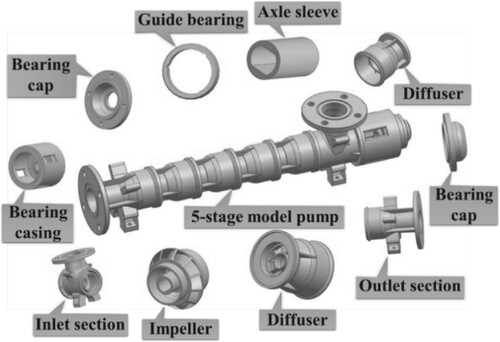
The research project for this study is a five-stage mixed-flow ESP. The research project’s 3D design, which includes the pump body, impellers, diffusers, and caps, is shown in Figure 1. Since the mixed-flow submersible electric pump works in deep wells, the radial dimensions of each component should be strictly controlled to reduce the cost. Based on the velocity coefficient method, the dimensions of the submersible oil electric pump are initially determined. The model pump uses three-dimensional twisted mixed-flow vanes with small radial dimensions and large axial dimensions of the space guide vane as the pressure chamber and adopts an annular suction chamber to achieve the real situation that water gushes into the impeller inlet uniformly from all around. In addition, the pump from the deep well pumping liquid, in the process of turning pumping, the liquid has a large amount of gas overflow. Therefore, the selected impeller vane number is 11. The increase in the number of vanes increase the vane inlet at the discharge coefficient, making the inlet flow velocity increases, and the bubbles with the high-speed liquid flow are pumped out of the impeller. The selected guide vane number and impeller vane number mutually reduce the impact loss on the guide vane inlet and impeller outlet.

Figure 1. ESP model.

2.2. Computational domain and meshing

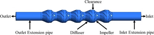
Figure 2 depicts the 3D modelling of the various computation domain of ESP using CREO Pro/E. The fluid computation domain model is reduced into four components by preserving the intake portion as a straight pipe: water inlet, rotor, guide vanes/diffuser, and outflow chamber. The lengths of the water intake and outflow sections are adequately expanded to enable the complete development of the flow.

Figure 2. Computation-domain of ESP.

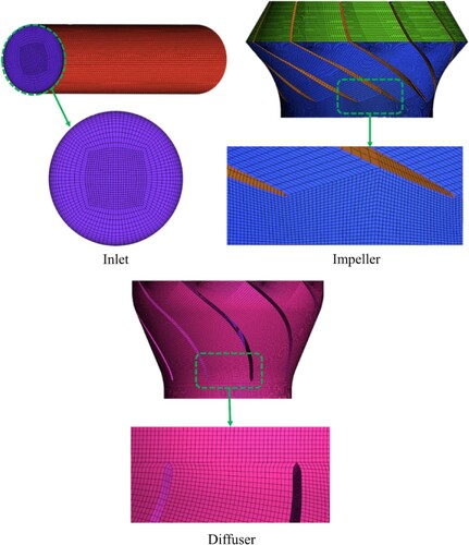
The ANSYS ICEM CFD tool is utilized to create hexahedral structured grids for the computational domain, encompassing components such as the guided vane, rotor, and sections for inlet/outlet extensions. In addition, the moving boundaries have been handled using the slip grid meshing approach. Figure 3 provides information on the various mesh cross-sections for all the computation domains.

Figure 3. Meshing grid of the computational domain.

2.3. Grid-independence analysis

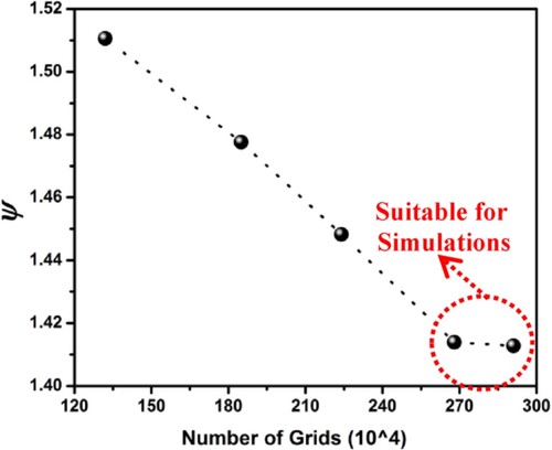
To minimise or completely eradicate the impact of the quantity of mesh components on the computing outcomes, the computational domain is subjected to the mesh independence analysis. Grid elements are selected based on head variations, and 1-stage ESP is analyzed using 5 distinct grid elements, maintaining fixed-values at nominal conditions. The comparison of head variations due to mesh elements is shown in Figure 4. Relevant literature (Li et al., 2020b; Si et al., 2019b) made the observation that the grid-elements’ impact might get disregarded if the inaccuracy of the projected values of heads beforehand and afterwards is less than 2%. Figure 4 shows that the model pump’s head change controls itself within 2% once the grid-components are bigger than 2.68-million. Consequently, 2.68 million meshes are selected for simulating a single-stage pump. However, in case of five-stage ESP, the grid assembly is realised in CFX-Pre by using translating commands, and the total number of grids is 13.34 million for conducting numerical simulation on five-stage ESP. Moreover, the head coefficient used in this Figure has been evaluated using the formula provided in Section 3.4 (Equation 16).

Figure 4. Mesh independence Analysis.

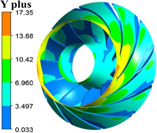
2.4. Validation of y+ parameter

To verify that the wall boundary layer thickness is within the acceptable range under the turbulence model, the parameter y+ is also examined. The research by Chen et al. (2021) and Zhang et al. (2021) provide the expression and description of y+, whereas Figure 5 provides the value of y+. Based on the findings of CFD calculations, when employing 2.68 million lattices, the y+ value near the impeller walls is just above 17 which align well with the requirements of the turbulence model.

Figure 5. y⁺ assessment at impeller wall.

2.5. Turbulence modelling (Standard k–ε model)

The k–ε model is chosen for numerical calculation of the performance characteristics of single-phase conditions. The turbulent model k–ε consists of two equations: one for turbulent kinetic energy (k) and another for turbulent dissipation (ε), as illustrated in the following equations. (1) $\begin{array}{rl}& \frac{\mathrm{\partial }\left({\rho }_{l}k\right)}{\mathrm{\partial }t}+\frac{\mathrm{\partial }\left({\rho }_l{u}_{j}k\right)}{\mathrm{\partial }{x}_j}=P_t-{\rho }_lϵ+\frac{\mathrm{\partial }}{\mathrm{\partial }{x}_j}\left[\left(\mu +\frac{{\mu }_t}{{\sigma }_k}\right)\frac{\mathrm{\partial }k}{\mathrm{\partial }{x}_j}\right]\end{array}$(1) (2) $\begin{array}{rl}& \frac{\mathrm{\partial }\left({\rho }_lϵ\right)}{\mathrm{\partial }t}+\frac{\mathrm{\partial }\left({\rho }_l{u}_jϵ\right)}{\mathrm{\partial }{x}_j}=C_{ϵ1}\frac{ϵ}{k}{P}_t-C_{ϵ2}{\rho }_l\frac{{ϵ}^2}{k}\\ & +\frac{\mathrm{\partial }}{\mathrm{\partial }{x}_j}\left[\left(\mu +\frac{{\mu }_t}{{\sigma }_{ϵ}}\right)\frac{\mathrm{\partial }ϵ}{\mathrm{\partial }{x}_j}\right]\end{array}$(2) (3) $\begin{array}{rl}& {\mu }_t=\frac{c_{\mu }{\rho }_m{k}^2}{ϵ}\end{array}$(3) where the model constants are $C_{ϵ1}=1.44$, $C_{ϵ2}=1.92$, ${\sigma }_{ϵ}=1.3$, ${\sigma }_k=1.0$, $c_{\mu }=0.09$, $P_t$ for the turbulent kinetic energy generation terms, respectively; ${\mu }_t$ is the turbulent viscosity coefficient, is a function of $k$ and $ϵ$; where ε is the turbulent dissipation rate (m²/s²), $c_{\mu }$ is the empirical coefficient, and $k$ is the turbulent kinetic energy (m²/s²).

2.6. Multi-phase flow models

2.6.1. Heterogeneous flow model (Eulerian)

A complex multiphase flow model suitable for calculations requiring complicated interactions within two-phase flows is the Euler-Euler model. Generally speaking, air is considered to be the discrete phase and water to be the continuous phase. Each phase fluid needs to have its own energy and continuity equation, and the fluids must interact with one another to balance the expression.

The continuity formula can be represented as (Si et al., 2018): (4) $\begin{array}{r}\frac{\mathrm{\partial }}{\mathrm{\partial }t}\left({\alpha }_k{\rho }_k\right)+\mathrm{\nabla }\cdot \left({\alpha }_k{\rho }_k{w}_k\right)=0\end{array}$(4) Whereas the energy equation is represented as: (5) $\begin{array}{rl}& \frac{\mathrm{\partial }}{\mathrm{\partial }t}\left({\alpha }_k{\rho }_k{\mathit{w}}_k\right)+\mathrm{\nabla }\cdot \left({\alpha }_k{\rho }_k{\mathit{w}}_k\otimes {\mathit{w}}_k\right)\\ & =-{\alpha }_k\mathrm{\nabla }{p}_k+\mathrm{\nabla }\cdot \left({\alpha }_k{\mu }_k\right(\mathrm{\nabla }{\mathit{w}}_k+\left(\mathrm{\nabla }{\mathit{w}}_k{)}^T\right))\\ & +{\mathit{M}}_k+{\alpha }_k{\rho }_k{\mathit{f}}_k\end{array}$(5) Where, $k$ is a variable that represents any phase, whether it be liquid or gas; ${\rho }_k$ represents the phase density, measured in kilograms per cubic metre; $p_k$ represents the pressure of the phase (Pa). ${\alpha }_k$ represents the phase volume-fraction. ${\mu }_k$ represents dynamic viscosity of phase. $f_k$ represents the rotational mass-force of impeller, measured in newtons (N). $M_k$ represents the Phase forces, (N). ${\mathit{w}}_{\mathit{k}}$ represents the fluid-phase relative-velocity, (m/s).

2.6.2. Vof (Volume of fluid model)

The Eulerian technique for simulating immiscible continuous phases is called the Volume of Fluid (VOF) method. In this model, the equations for mass and momentum conservation in the presence of particles are provided in references (Hirt & Nichols, 1981; Kumar et al., 2021), and represented as follows, (6) $\begin{array}{rl}& \frac{\mathrm{\partial }}{\mathrm{\partial }t}\left({\alpha }_k{\rho }_k\right)+\mathrm{\nabla }\cdot \left({\alpha }_k{\rho }_k{w}_k\right)=0\end{array}$(6) (7) $\begin{array}{rl}& \frac{\mathrm{\partial }}{\mathrm{\partial }t}\left({\alpha }_k{\rho }_k{\mathit{w}}_k\right)+\mathrm{\nabla }\cdot \left({\alpha }_k{\rho }_k{\mathit{w}}_k{\mathit{w}}_k\right)\\ & =-{\alpha }_k\mathrm{\nabla p}+\mathrm{\nabla }\cdot \left({\alpha }_k\tau \right)+{\alpha }_k{\rho }_{k}g+{\mathit{f}}_{\mathrm{\sigma i}}-{\mathit{F}}_{\mathrm{pk}}\end{array}$(7) In these equations, $\tau$ represents fluid stress tensor, $g$ represents gravitational acceleration, ${\mathit{f}}_{\mathrm{\sigma i}}$ represents surface tension force, and ${\mathit{F}}_{\mathrm{pk}}$ represents the transfer of momentum across Eulerian and Lagrangian phases. In this instance, ‘${\alpha }_k$’ denotes the proportion of fluid (including both gas and liquid) in terms of volume, represented as; ${\alpha }_k={\alpha }_g+{\alpha }_l$.

The variables ${\alpha }_g$, and ${\alpha }_l$, represent volume fraction of gas and liquid, respectively. At the gas – liquid interface, thermophysical characteristics can be measured using weighted averages. (8) $\begin{array}{rl}{\rho }_k& ={\alpha }_g{\rho }_g+{\alpha }_l{\rho }_l\end{array}$(8) (9) $\begin{array}{rl}{\mu }_k& ={\alpha }_g{\mu }_g+{\alpha }_l{\mu }_l\end{array}$(9) The CSF (continuum surface force) model (Brackbill et al., 1992) is used to calculate the surface tension force ${\mathit{f}}_{\mathrm{\sigma i}}$ at the gas – liquid interface. (10) $\begin{array}{r}{\mathit{f}}_{\mathrm{\sigma i}}=\frac{\mathrm{\partial }{\alpha }_g}{\mathrm{\partial }{x}_i}\left(\mathrm{\sigma K}\right)\end{array}$(10) Moreover, the curvature, represented as K, can be computed as, (11) $\begin{array}{r}K=-\frac{\mathrm{\partial }{n}_i}{\mathrm{\partial }{x}_i}=-\frac{\mathrm{\partial }}{\mathrm{\partial }{x}_i}\left[\frac{\mathrm{\partial }{\alpha }_g/\mathrm{\partial }{x}_i}{|\mathrm{\partial }{\alpha }_g/\mathrm{\partial }{x}_i|}\right]\end{array}$(11) In Equation (7), ${\mathit{F}}_{\mathrm{pk}}$ represents the transfer of momentum between the Eulerian phases (liquid and gas) and the Lagrangian phase (particle), and the gas volume fraction, ${\alpha }_g$, is calculated by solving the equation. (12) $\begin{array}{r}\frac{\mathrm{\partial }{\alpha }_g}{\mathrm{\partial }t}+\mathrm{\nabla }\cdot \left({\alpha }_g{w}_k\right)+\mathrm{\nabla }\cdot \left[{\alpha }_g\left(1-{\alpha }_g\right)w_c\right]=0\end{array}$(12) The relative velocity among the gas and liquid phases is shown by the artificial compressive velocity $w_c$.

2.7. Cfd setup and boundary condition setting

The three primary steps of the CFD setup are CFX-Pre, CFX Solver, and CFX post-processing. Figure 6 illustrate how the fully constructed computational domains of pump are assembled in Ansys CFX pre. The boundary conditions, which are covered in later sub-section, are denoted by pointing arrows (arrows pointing inwards and outwards are indicating the inlet and outlet, respectively).

Figure 6. Fully constructed computational domain of ESP in ANSYS CFX-Pre.

2.7.1. Boundary conditions

The CFD calculations of the fluid flow must include boundary conditions, which are a collection of characteristics or requirements on the surfaces of computational domains. Therefore, the selection of appropriate boundary conditions is essential for running two-phase flow simulations. The following boundary conditions are mainly included for the ESP simulation.

The flow field calculation domain of ESP is numerically computed using ANSYS 18.1 software. The calculating domain is partitioned into several regions, including the stationary regions such as the straight intake pipe, the clearance, the diffuser, the outlet, and the rotating region of the impeller. The working medium is pure water at room temperature. The simulated rotational speed is configured to 1475 rpm, while the operational flow rate Q_d is set to 7.5 m³/h. For steady-state simulations, the flow between the impeller, volute, and output pipe is calculated using the ‘frozen-rotor’ interface. The volute and outlet pipe domain are assigned as a static frame of reference, while the rotor-domain is assigned as a rotating-region. The boundary conditions for the inlet and outlet are static pressure (1atm) and bulk mass flow rate, respectively. The ESP simulation utilizes the conventional k-e turbulence model. The general grid interface (GGI) mesh connection is applied to provide a complete link between grids that do not match and have varied pitch angles on neighbouring surfaces. The wall roughness boundary condition for all parts except inlet and outlet pipes are set as a rough wall with the roughness value of 0.01 mm for plastic material, whereas the setting of mass and momentum is selected as no slip wall.

Since the two-phase flow characteristics of the fluid is complex and turbulent, and the steady simulations could not well predict the flow behaviour within the ESP. Therefore, we have conducted an unsteady simulation to obtain the complete multiphase flow features of ESP that can be fairly equal to real time test results. For unsteady simulations, the impeller-volute interference has been updated as ‘Transient rotor-stator.’ The reason is because with this kind of interface, the relative position between the impeller and volute varies with each time step. The time step for unsteady simulation is 3.38983 × 10⁻⁴ s, equal to 3° of impeller rotation. The impeller is rotated for four full rotation periods, which takes a total time of 0.1627 s in total. The maximum convergence coefficient control loops are selected for each time step, and the maximum number of control loops was set at 25 to achieve convergence. The temporal discretization method used is the second-degree backward Euler transient technique. The convergence residual type chosen is the root-mean-square (RMS), with a target of 10⁻⁴. All the unsteady computations were resolved for three distinct flow rates (0.8Q_d, 1.0Q_d, 1.2Q_d).

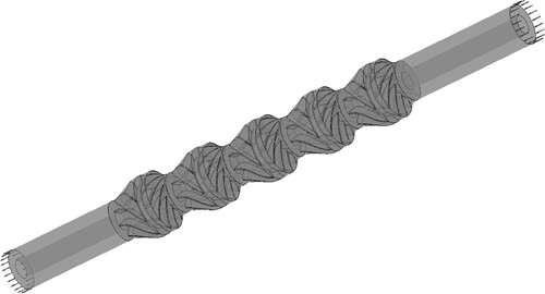
3. Experimental methodology

In contrast to actual power plant setups, this study has used an open-loop test facility in the research centre (refer to Figure 7a) to test the prototype ESP’s capability to handle two-phase flow. The pump is driven by splined shafts, and the housings of four elements are flanged. The experiments follow a multi-stage mixed flow ESP setup. The pump’s multi-phase performance was tested in the lab using a five-stage ESP and a helical tube is designed to simulate actual pump input conditions. Tap water and air serve as the fluid-materials, reflecting the liquid and gas phases independently. The water/air were used instead of petroleum fluids for practical reasons in experimentation in order to follow safety measures and the laboratory rules and regulations. Table 1 shows the designed/operational factors of pump model. As the oil-gas separator pump configurations in power plants would limit the entry of IGVFs by a maximum of 15%. Thus, up to 14% of GVFs were studied in the present gas–liquid two-phase flow studies. Furthermore, Figure 7b and c depicts the interstage assembly and air admission device, respectively. However, the space between the diffuser intake and the impeller exit is represented by the clearance in Figure 7b.

Figure 7. Complete arrangement of ESP system. (a) Complete arrangement of ESP installation within laboratory. (b) inter-stage assembly of ESP. (c) Air admission device.

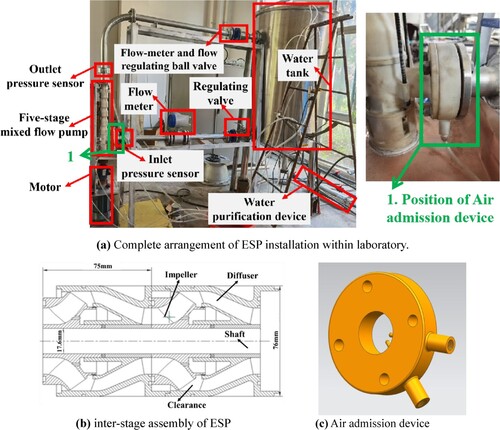
Table 1. Designed parameters of the prototype pump model.

Category	Factor	Symbolization	Unit	Value
Impeller and diffuser	Impeller diameter (outlet)	D2	mm	67
	Impeller diameter (inlet)	D1	mm	45.7
	Blade outlet-width	b2	mm	6.24
	Impeller blade number	z	-	11
	Diffuser blade number	-	-	9
	Pump inlet diameter	d1	mm	50
	Pump outlet diameter	d2	mm	50
	Blade, diffuser wrap angle		^o	70, 70°
Operational Condition	Designed flow rate	Q	m^3/h	15
	Rotating speed	n	r/min	2950
	Specific speed $n_s=n\sqrt{\mathrm{Qd}}/H^{3/4}$	$n_s$	-	304.9
	Designed Head	H	m	15

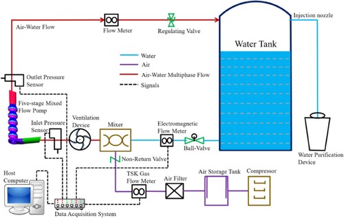
3.1. Experimental loop and equipment

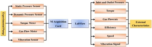
The following test configuration (Refer to Figure 8) was used to carry out flow-performance measurements of model pump under both single – and two-phase operations. The test flow-loop consists of the following components: the several control valves and pipes, the NI USB-6343 acquisition card, the LabVIEW acquisition programme, the host computer, the air-container, the air-compressor, the ventilation device, the gas delivery-circuits, the water-container, the electromagnetic flow-meters, the Bürkert gas flow-controller, the air-compressor, the torque-metre, and the motors. Figure 8 depicts the experiment configuration for the multiphase-flow studies.

Figure 8. Diagrammatic representation of the ESP operating under multiphase flow test system.

3.2. Test arrangement and acquisition system

The primary tools used in the studies are an NI USB-6343 acquisition card and an acquisition-programme developed in LabVIEW software, which together allows for immediate identification and collection of experimental data. The gathered data findings are stored in the designated directory in Excel format. Figure 9 depicts the full test-data collecting procedure.

Figure 9. Complete acquisition-process of signal acquisition.

3.3. Test uncertainty measurements

Experimental results obtained at various periods may not be the same due to challenges with experiment reproducibility, variations in environmental circumstances, and a lack of understanding among researchers (Sun et al., 2018). There is a large range of deviation in the findings. Uncertainty analysis may be used to find such a divergence. It isn’t used to assess how well the computed data matches the real data.

The ISO 9906:2012 standard was followed to acquire the head and global efficiency of the pump performance study. This standard allows for an error value of 1.5% for head and power determination and 2% for flow rate measurements. The tests were carried out under the specified operating circumstances, and the comparable calculation approach described by (Sun et al., 2018) was used to determine the uncertainty values. The error in the measurement was calculated to be 0.2% for IGVFs, 0.1% for rotational speed, 1.2% for the pump head, and 2.4% for hydraulic efficiency.

3.4. Test outcomes and assessments

The display evaluation of the ESP system’s performance is determined through the use of the mathematical expression given as (Ali et al., 2022a, 2023): (13) $\begin{array}{r}\eta =\frac{\mathrm{\rho gQH}}{\mathrm{\tau \omega }}\end{array}$(13) Equation (14) is used to calculate the theoretical head (H) in terms of the total pressure increase in ESP. (14) $\begin{array}{r}H=\frac{P_2-P_1}{\rho \mathsf{g}}+\frac{V_2^2-V_1^2}{2\mathsf{g}}+\left(Z_2-Z_1\right)\end{array}$(14) In the given equation, H represents the head imposed by the ESP into the working medium. P1 and P2 denote the static pressures measured by the pressure sensors at the inlet and outlet of the ESP, respectively. At the inlet and outlet sections of the ESP, V1 and V2 represent the mean flow velocities of the fluid, respectively. The parameters Z1 and Z2 represent the vertical distances from the central point of the inlet and outlet sections of the ESP to the plane where the pressure sensor is positioned at the inlet and outlet, respectively.

The outcomes characteristics of electric submersible pump were determined under circumstances of two-phase flow. The pump was operated at a rotational speed of 1475 revolutions per minute (r/min) while varying the flow rates. At high rotational speed it was challenging to shut the valve and achieve a low flow rate throughout the testing. As a result, the acquisition of experimental data at higher rotational speeds is not possible under two phases flow conditions. The other main factor contributing to the issue was the use of acrylonitrile–butadiene–styrene copolymer (often referred to as ABS resin) as the production material. Additionally, tiny size of the pump made it vulnerable to breakage when exposed to gas, particularly owing to the increased pressure in the pump outlet resulting from greater rotating speeds.

The flow rate and head coefficients are dimensionless variables that are primarily used to estimate the performance changes of a pump operating under varied flow circumstances or two pumps with comparable design characteristics. Furthermore, the flowrate, head, and two-phase theoretical head coefficients are calculated as follows; (15) $\begin{array}{rl}\phi & =\frac{Q}{2\pi R_2{b}_2{u}_2}\end{array}$(15) (16) $\begin{array}{rl}\psi & =\frac{\mathrm{gH}}{u_2^2}\end{array}$(16) (17) $\begin{array}{rl}{\psi }_{\mathrm{tp},\mathrm{th}}& =\frac{{\psi }_{\mathrm{tp}}}{\eta }\end{array}$(17)

The variables H, Q, and u_2 represent the head, flow rate, and circumferential velocity at the impeller tip, respectively.

3.4.1. Performance curve of ESP for water

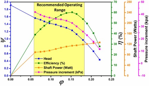
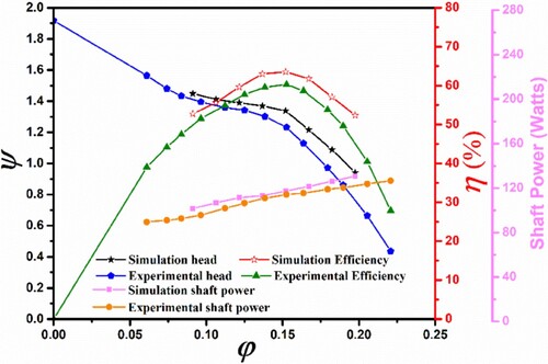
The efficiency graph of ESP operating in pure water at a rotational speed of 1475 rpm is shown in Figure 10. The pump’s operating capacity remains constant despite variations in flow rate, as per the Euler equation. On the other hand, based on real-time experimental findings, a progressive deterioration in pump performance is seen as flow rate increases. The characteristics graph for ESP operating in pure water at a rotational speed of 1475 rpm is shown in Figure 10. The pump’s operating capacity remains constant despite variations in flow rate, as per the Euler equation. On the other hand, based on real experimental findings (refer to Figure 10), a progressive deterioration in pump performance is seen as the flow rate increases. When the ESP functions at no flow rate condition, the maximum head value is about two times bigger than the needed Head (H_d), whereas the highest flow rate value that may give a suitable head is marginally higher at 1.4Q_d. The pump’s BEP at the nominal flow rate of 7.5 m³/h is 60.3%, which is the greatest possible efficiency. The aforementioned process may be explained as follows: when the flow rate increases, turbulent flow within the ESP impeller causes hydraulic losses that impede the ESP’s capacity to function.

Figure 10. ESP’s performance characteristic curve in single-phase flow environment.

3.4.2. Characteristics curve of ESP for gas contents

The performance curves of an ESP operating at 1475 rpm rotational speed under various flowrates and inlet gas volume fractions (IGVFs) are shown in Figure 11. With the exception of a compressor connected next to the intake to inject gas into the ESP, the test parameters and conditions for the two-phase flow were the same as those for the single-phase flow. Numerous IGVFs are used and investigated.

Figure 11. ESP’s performance characteristic curve in the presence of two-phase flow circumstances.

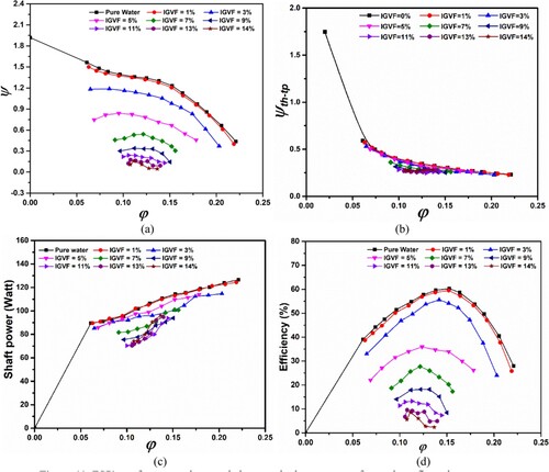
As shown in Figure 11a, the ESP has amazing gas-controlling capabilities. Because earlier research (Si et al., 2018) showed that as IGVFs get close to 3% or higher, pump efficiency starts to decline. Thus, as IGVFs rise for a given flow characteristics curve, both flow-rate and head decrease. At smaller amounts of IGVFs (<4%), the performance results show only slight fluctuations, which may be the result of compression among all five-stages of ESP. However, when the IGVFs are between 4% and 14%, an apparent reduction in pump performance could be observed. Furthermore, when the flow coefficient ranges from 0.017 to 0.021, the maximum value of IGVF is around 14%. This value was achieved without experiencing pump surging. The above flow coefficient values correspond to volume flow rates between 5.54 and 6.83 m³/h. These values are closely associated with the Best Efficiency Point (BEP) achieved at Q_d = 0.023, specifically under pure water circumstances.

Figure 11b validates the idea of apparent losses by demonstrating that the theoretical head coefficient curve remains constant regardless of the input void percent (up to 9%). Figure 11b illustrates that the onset of higher degradation in ESP is linked with a certain flow coefficient that corresponds to the transition from a constant negative slope of the theoretical head coefficient. Under a flow coefficient of 0.08, the predicted head curve deviates from a linear relationship. This observation suggests that there is no swirling flow at the intake and that the outlet flow angle at the rotor’s exit plane remains steady.

Furthermore, Figure 11c shows the impact of IGVFs on the use of shaft power. The figure illustrates that when the flow rate increases, the shaft power value exhibits an upward trend for both single and two-phase flow circumstances. Nevertheless, the rise in IGVFs causes a slowdown in the pump’s rotational speed, resulting in a decrease in the amount of shaft power needed by the pump. This observation is supported by Yaqob and Abbas (2009). This might be due to several losses produced by the unsteady flow, recirculation, and vortex structures under two-phase flow, resulting in lower efficiency for the two-phase flow conditions.

Figure 12 shows the performance characteristics curves at different IGVFs as well as at different flow conditions (0.8Q_d, 1.0Q_d, 1.2Q_d). For the sake of simplification, all the results in Figure 12 are represented using head ratio (H/H₀), efficiency ratio (η/η₀), and shaft power ratio (Sp/Sp₀). Where, H₀, η₀, and Sp₀ represents the values of head, efficiency and shaft power under pure water conditions (IGVF = 0%). Pump performance characteristics are less affected by changes in flow rate when the IGVFs are less than 4%. As IGVFs grow, the pump performance decreases linearly. However, when IGVFs rise to >4%, the head decreasing curve declines more rapidly, and the impact of IGVF on pump performance increases as flow rate circumstances shift from design to off-design circumstances. When the Gas content is 4% and 5%, the pump suffers a sudden head drop, highlighted as green dashed circle (See Figure 12a). This stage of sudden drop in pump performance is regarded as surging initiation point. Similar outcomes have been previously observed and validated by Sato and Furukawa (2010).

Figure 12. Head characteristic curve of ESP at different flow rates under two-phase flow conditions.

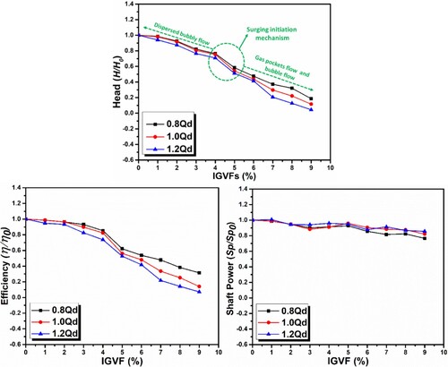
Under the least value of flow rate (0.8Q_d condition), the pump exhibits the maximum values of head at all values of IGVFs, which are minimum in case of 1.2Q_d condition (overload condition). This reveals the fact that the more the flow rate, the more H/H₀ and η/η₀ decrease but exhibit the same surging position. Moreover, further increase in the IGVFs (>5%) cause a sudden decrease in pump performance and the head descending curve becomes more irregular. It is only because of the unsteady flow, recirculation, and vortex structures under two-phase flow, resulting in lower performance of ESP. Furthermore, all the values such as head, efficiency and shaft power in Figure 12 have been taken at the value of total flowrate. That’s why, the shaft power curve is almost constant (See Figure 12c).

Since the two-phase flow behaviour of the fluid is complex and turbulent, the steady simulations could not well predict the flow behaviour within the ESP. Therefore, all the CFD-simulation outcomes have been achieved through an unsteady simulation to obtain the complete two-phase flow features of ESP that can be fairly equal to real-time test results. The Euler-Euler heterogeneous two-fluid model is used for computational fluid dynamics (CFD) calculations to simulate the performance and internal flow patterns in an impeller flow (ESP) under different (IGVFs). This model assists in understanding the complex flow behaviour of the fluid within the impeller flow passage. The results obtained from the Euler-Euler model simulation are subsequently compared and validated with the experimental results.

4. Results and discussion

4.1. CFD results for single-phase flow

4.1.1. Validation of CFD results

The comparison of test data and numerical outcomes on ESP performance results under pure water circumstances (at a rotational speed of 1475 rpm) is shown in Figure 13. To comprehensively examine the fluctuating pattern of energy efficiency across different flow rates, a numerical simulation was conducted using a total of eight running flow rates ranging from 0.6 Qd to 1.3Q_d.

Figure 13. Comparison of experimental and numerical results.

The figure reveals that the simulated values of the head and efficiency curves are marginally greater than the experimental values. However, the performance curves obtained through numerical calculations and experiments are essentially identical. The optimal efficiency point is found at a flow rate of 7.5 m³/h, which is equivalent to 1.0Q_d. The relative error of each curve exhibited an upward trend in the region where it deviated from the design flow rate. This was primarily caused by the occurrence of severe turbulence and backflow in the ESP operating within this region, as well as the losses resulting from the contact between the rotating blade and stationary diffuser. Consequently, the error between the numerical simulation and the experimental results increased. Furthermore, the numerical calculation procedure simplifies the model calculation domain, which may contribute to the discrepancy between the estimated value and the experimental value. Nevertheless, the inclination of each comparable curve was almost identical. The relative errors of the head, efficiency, and power between the numerical calculation and the test results were 1.08%, 3.2%, and 3%, respectively, under the design flow rates. The relative errors for all curves were below 5%, indicating that the numerical simulation approach used in this research is generally accurate and consistent.

4.1.2. Static pressure distributions

Figure 14 displays the distribution of static pressure at all stages of the ESP under both design and off-design situations. Since the multistage ESP is constructed for achieving the higher-pressure head. Therefore, the static pressure is increasing along different stages of ESP, exhibiting the maximum at the last stage of ESP (See Figure 13 for all flowrate circumstances).

Figure 14. Static pressure contours of ESP at single-phase flow.

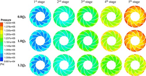
The static pressures are smoothly distributed within the ESP impeller for different water flowrates (0.8Q_d, 1.0Q_d, and 1.2Q_d) and for all stages. However, it shows a gradual increasing trend from leading edge to the trailing edge of the vanes, showing the lowest close to the suction side (indicating occurrence of cavitation) and the maximum near the blade outlet and diffuser inlet (produced due to rotor-stator interaction) (Ali et al., 2022b) in the circumferential direction. The flow separation area inside the rotor flow passage should be positioned in low-pressure regions, such as the area around the suction side of the blades. This separation area leads to flow losses within the impeller flow channel, as mentioned in reference (Si et al., 2019b), which ultimately causes a decrease in the performance of the ESP.

4.1.3. Flow field velocity streamlines

Figure 15 represents the velocity streamline distribution in centre of the rotor flow channel of ESP under design and off-design circumstances. As can be seen, the streamline distribution varies dramatically between the three simulated situations (0.8Q_d, 1.0Q_d, and 1.2Q_d). The streamlines are uniform inside the ESP impeller for high water flow rate conditions. However, when the water flow rate is low (designed condition, 1.0Q_d), the flow is uniformly distributed inside the whole flow passage but the smaller vortex and recirculation occur around the leading edge of the impeller blades.

Figure 15. Velocity streamline distribution of ESP at single-phase flow.

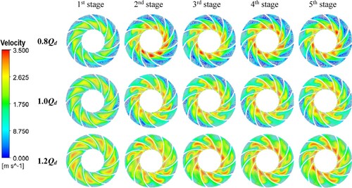
At this flow point, an obvious vortex produced on the trailing-edge of blades (impeller outlet) but it’s not so strong. As the flow velocity of the water lowers more (0.8Q_d), the vortex grows larger and stretches almost all the way to the outlet. The flow disturbances in the impeller flow channel are caused by these vortices and secondary flows inside the revolving ESP impeller. which in turn severely disrupt the impeller’s input flow conditions.

4.2. CFD results for two-phase flow

4.2.1. Comparison of multiphase flow models

For the operating condition at n = 1475 r/min and Q = 7.5 m³/h (φ = 0.152), Figure 16 compares the simulation and test results of the efficiency features of ESP under various IGVFs. Two distinct multiphase flow models – the VOF model and the Euler-Euler two-fluid model – are used to compare the numerical findings. Additionally, both head and efficiency are shown in their non-dimensional forms for convenience of comparison; for example, head ratio as (H/H₀) and efficiency ratio as (η/η₀), where and are the values of head and efficiency under pure water circumstances, respectively.

Figure 16. Comparative analysis between Two different multiphase models.

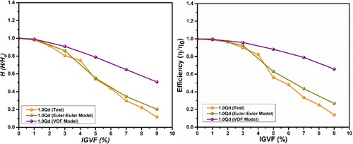
Figure 16 illustrates that as IGVF increases, the head and efficiency ratios determined by numerical calculations and experimentation both eventually decline. Furthermore, the numerical findings of the Eulerian model are more in agreement with the actual results for higher levels of IGVF (6–9%). This is because, under small IGVF, bubbles coalesce and break at a slower rate than under large IGVF, then bubbles collide, they create a liquid film on the surface and they come into contact with. The film converges as the diameter of the bubble reaches a specific threshold, resulting in the formation of two or more bubbles.

Regarding the comparison between VOF and Euler-Euler model, the Eulerian model yields lower head and efficiency values than the VOF model. Additionally, the CFD simulated graphs and patterns by Eulerian-Eulerian conventional model are highly reliable and consistent with experimental observations. This is due to the fact that the VOF model is not good at capturing the phase slippage inside the rotating ESP impeller. Secondly, the transient Eulerian-Eulerian multiphase model is superior to VOF model in studying gas–liquid two-phase flow and bubble dynamic behaviours inside ESPs. Consequently, the Eulerian model will be used as the two-phase flow model for the calculation of gas–liquid multiphase flow in the future.

4.2.2. Validation of CFD results on two-phase flow

Figure 17 illustrates a comparison of simulation and experimental outcomes for ESP performance at various IGVFs and flow rates. According to Figure 17a, the simulation findings follow the same pattern as the test results for different IGVFs, and under situations of gas–liquid two-phase flow, the head values were consistently less than those of pure water flow. The head attained its highest value at the nominal flowrate (Q_d= 7.5 m³/h, φ = 0.152) under different IGVF conditions, which is distinct from the pure water circumstances. However, under off-design conditions, the pump’s performance was strongly impacted by the inlet gas composition.

Figure 17. Comparison of test and simulation performance curves under two-phase flow. (a) Head; (b) Efficiency; (c) Shaft power.

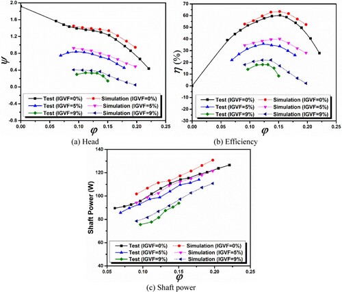
Figures 17b and c demonstrate the efficiency and shaft power at various IGVF conditions, respectively. The curve of each parameter increases with the increase in flowrate, and it is comparable to flowrate and head curve. The ESP’s excellent efficiency range was constrained as the IGVFs increased, and under over-load situations, efficiency quickly decreased. This is might be because the flow patterns are altered in the impeller channels under the multiphase flow situation (Li et al., 2020a). When the gas concentration reaches a specific level (IGVF = 9%), the smaller bubbles accumulate to form bigger bubbles, causing gas blockage in the impeller channels (Cubas et al., 2020). At this stage, the transition happened transitioning from a bubbly flow to an expanded bubble flow, resulting in a strong decline in head and efficiency of ESP.

4.3. Complex internal flow analysis under two-phase flow

The CFD results of ESP at each-stage rotor in both two-phase and pure water flow circumstances are shown in Figure 18. The multiphase flow graphs were acquired at the designed flowrate (Qd = 7.5 m³/h, φ = 0.152) and various IGVF values. According to Figure 18a, it can be observed that all stages reflect identical performance, except for the first-stage impeller, which features a higher head compared to the other stages. The uniform distribution of flow from the inlet suction pipe without any pre-rotation allows for the incoming flow inside the first-stage impeller is well-oriented. However, the flow inside the second and other stages is affected by swirls (disoriented flow) beginning from the first-stage diffuser and other return channels. Because of this, the head of the first-stage impeller is higher than that of the other four stages. The previously described occurrences were supported by Stel et al. (2015), and Ofuchi et al. (2017).

Figure 18. Simulated outcomes for ESP-performance on each stage impeller. (a) pure water condition; (b) two-phase flow conditions when Qd = 7.5 m³/h (φ = 0.152).

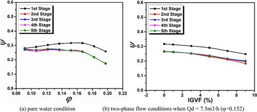
Furthermore, Figure 18b indicates that the final four-stages of ESP noticed the greatest performance deterioration, and all stages exhibit a similar declining pattern as IGVFs grow. Upon carefully examining Figure 18b, the following general inferences may be made: Before to moving on to further stages, the initial step seems to function as a pre-mixer, enabling the bubble sizes to be smaller and more uniform. This is further supported by the CFD findings and further emphasized in the second and subsequent phases. This indicates that to achieve optimal and evenly dispersed homogenous flow conditions, a multistage arrangement may need at least 4 or 5 stages. Furthermore, by examining the internal flow analysis, which includes the gas void-fraction distribution, velocity streamlines and vortex structures (will be discussed in the subsequent sections) it is possible to fully comprehend the cause of the most noticeable and unique performance decline of ESP. According to the outcomes observed in Figure 18, the performance of first-stage impeller is the most prominent case to be analysed. Therefore, all the following analysis are conducted only on the first-stage impeller to evaluate the actual reason behind the distinct behaviour of first stage compared to other stages of ESP.

4.3.1. Gas distribution in ESP

Distinct IGVFs have different impacts on the ESP performance. As the IGVFs grow, the proportion of gas in the rotor flow channel also increases, which hinders the smooth flow of liquid-phase. Once the IGVF hits a certain threshold, the impeller channels experience the gas lock phenomena, resulting in a significant deterioration of the pump’s operational stability. Figure 19 illustrates the gas distribution on the centre cross-section of the 1st stage impeller for three distinct IGVFs (1%, 5%, and 9%) and flowrate settings (0.8Q_d, 1.0Q_d, and 1.2Q_d). The impeller is moving counterclockwise, causing gas buildup on the suction side of the blade. This accumulation gradually builds up along the flow chamber of the impeller towards the output.

Figure 19. Gas distribution trend in middle section of 1st stage impeller of ESP at distinct IGVF and flowrate.

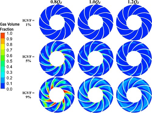
At an IGVF level of 1%, the presence of gas has a negligible effect on the operation of the ESP. Gas buildup is only seen along the suction surface, which is influenced by the pressure gradient around the edges of the impeller flow channel. Under these circumstances, the gas occupies a very limited fraction of the impeller, resulting in little effect on the main flow channel. Nevertheless, when the IGVFs reach a value of 5%, the gas buildup first increases in proximity to the suction surface and then spreads along the impeller blades, filling a portion of the impeller flow path. Currently, the gas bubbles occupy about 40% of the impeller flow channel for all three flow rates, indicating a greater amount of gas concentration under the part load condition (0.8Q_d). In addition, when the maximum value of the Internal Gas Volume Fraction (IGVF) is reached at 9%, there is significant growth in the build-up of bubbles inside the flow channel of the impeller. These bubbles are completely formed throughout most of the impeller hub and the rear of the blade, except the flow channel near the impeller outlet. Under these circumstances, some bubbles continue to grow in the radial direction of the impeller, obstructing up to 60% of the flow channel. This significantly impairs the hydraulic performance of the pump model (Ali et al., 2021; Qiaorui et al., 2022; Si et al., 2019a). Conversely, the gas distribution has diminished with varying IGVFs as the flow rate has risen, suggesting that the ESP is more responsive to gas at low flow rates. These variations modify the whole flow pattern of ESP, leading to a decline in pump efficiency.

4.3.2. Gas distribution under different impeller rotating angles

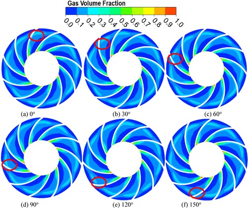
To study the behaviour of a gas under various rotating angles, the air volume distribution was treated to an unsteady flow-field investigation with an IGVF of 9% underrated flow conditions (1.0Q_d).

Figure 20 shows the amount distribution of the gas contents on the cross-section at various impeller angular positions. As the impeller rotated at different angles, the gas distribution within the flow passage of the impeller gradually changed. The majority of the gas phase was accumulated close to the blades’ suction surface, and it progressively diffused across the rotor flow passage in the direction of impeller’s outlet. With the gradual increase in impeller rotating angle (0°–150°), the phenomena of separation and agglomeration of air bubbles developed simultaneously around the direction of flow. The separation phenomena happened primarily close to the blade’s trailing edge on the rotor’s suction side, resulting in the drop of air bubbles from the blade outlet, which is then introduced in the diffuser domain.

Figure 20. Volume distribution of the gas contents on the first stage impeller’s cross-section at various rotational positions.

Note: Working conditions (IGVF = 9%, and 1.0Qd). (a) 0°; (b) 30°; (c) 60°; (d) 90°; (e) 120°; (f) 150°.

4.3.3. Velocity diagram and flow field

Figure 21 shows the distribution of gas velocity streamlines under three distinct flow rate settings (0.8Qd, 1.0Qd, and 1.2Qd) and IGVFs (1%, 5%, and 9%) in the centre region of the ESP’s first-stage impeller. It also signifies the impact of the flow rate on the gas velocity, which is evident and exhibits a positive association.

Figure 21. Gas velocity streamlines at the centre of 1st stage impeller of ESP at distinct IGVF and flowrate.

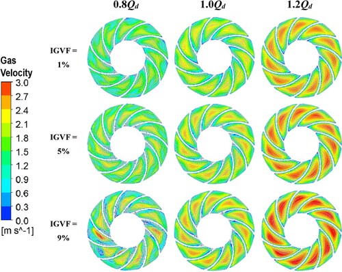
Figure 22 indicates that the gas flow streamlines are not very unstable and that there are some swirls in the flow channel, however, they are not very noticeable at design flow rate settings. However, at 0.8Qd circumstances, there are clear swirls and vortices inside the impeller flow channels, and the distribution of the gas streamlines is very erratic, particularly at the maximum IGVF (9%). The air velocities increase in the centre of the impeller hub, suggesting that swirl movement has a significant influence on the position and agglomeration of gas bubbles, which are capable of producing gas pocket formation and pressure surge, leading to the reduction in pump performance. Besides, an obvious increase in air velocity is can be seen with the increase in both IGVF and flow rates, indicating the good credibility of our simulation analysis on ESP (Zhou et al., 2020).

Figure 22. Vortex structures at the centre of 1st stage impeller of ESP at different IGVF and flowrate.

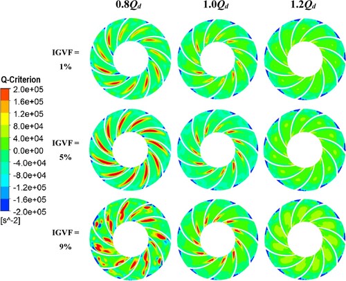
4.3.4. Influence of IGVFs on vortex distribution:

Generally, the multiphase flow inside the ESP is followed by the formation of swirls and vortices. These vortices are made up of a vortex field, which specifies how the vortices are distributed spatially. In ANSYS CFX, these transient vortex formations have been monitored using CEL (CFX expression language). We may designate inputs as variables, record results as variables, and control those variables by using CEL.

In addition, the Q-criterion is a useful tool for finding and visualizing vortex formations in complicated flow fields inside different turbomachines. The Q-criterion, introduced by Lilley (Hunt et al., 1988) in 1988, utilizes the positive area of the second matrix that contains the invariant Q of the velocity gradient tensor in the flow field to identify the existence of vortex formations. This criterion showed how fluid rotation and deformation in the flow field were balanced. For instance, when Q > 0 denotes that the fluid in the impeller flow channel is mostly rotating, and when Q < 0 indicates that the fluid is primarily deforming. The expression of Q-criterion is shown in the following: (18) $\begin{array}{r}\mathcal{Q}=\frac{1}{2}\left(\parallel B{\parallel }^2-\parallel A{\parallel }^2\right)\end{array}$(18) Where A, B represents the symmetric and asymmetric component of the velocity gradient tensor; and $||\cdot ||$ identifies the Frobenius parameter. Figure 22 is showing the cloud map of Q-value distribution in the middle section of the impeller at rated speed (1475 r/min) under three different IGVFs (1%, 5%, and 9%) and flow rate conditions (0.8Q_d, 1.0Q_d, and 1.2Q_d).

The Figure shows how the range of Q-values in the central area of the impeller suction surface rises with the increase of IGVFs and flow rates in the impeller runner. While the Q-value presented in the output region of impeller flow passage is lower for all values of different flow conditions, demonstrating that the change in Q-value influences how the vortex core is distributed in the impeller channel. Under different IGVF conditions, the formation of vortex in ESP is mostly related to the rotational motion of the impeller, and there is a significant energy loss in the vortex zone. In general, the Q-value distribution and the blade surface gas distribution are more uniform. The Q-value in the inlet region of the impeller flow channel is considerable with a certain correspondence, indicating that the rotation and strain of the small air bubbles in this location are not in equilibrium, resulting in flow instability in the impeller flow channel. It also suggests that the vortex has declined influence on the two-phase performance of pump model.

5. Conclusions

To examine the operational capability and unstable inner flow-field of the model pump, a numerical simulation technique for pure-water and two-phase flow is developed. The numerical simulations are based on Euler-Euler two-phase model, which is selected after comparing it with VOF model and test results. The CFD calculation of the ESP is carried out under different IGVFs and three flowrate conditions (0.8Q_d, 1.0Q_d, and 1.2Q_d). The outcomes demonstrate that:

1. In pure water, numerical findings indicate a decent agreement between the simulated and experimental values. When comparing the numerical calculation to the test results under the design flow rates, the head, efficiency, and power showed relative errors of 1.08%, 3.2%, and 3%, respectively, which is less than 5%, proving the credibility of the simulation method. Moreover, there are still some unwanted flows within the impeller flow channel, produced by vortices and flow separation, under design and part load conditions. The unstable flow (formed by impeller rotation) in impeller flow passages, on the other hand, generates a vortex flow, with the highest velocity created near the suction surface and around the impeller flow passage. As the impeller flow channel gets dispersed, the impeller outlet provides a high flow separation especially at part load conditions, reducing the operational capability of ESP.

2. Comparing the performance results of two phases throughout various experiments., Eulerian model, and VOF model demonstrated that the Eulerian model is in satisfied with the results and shows higher adaptability pattern with the test results. This reveals its best capability and versatility in predicting two-phase performance and internal flow results for the complex turbomachines such as ESP. Because, it can more accurately capture the phase slippage inside the pump model under for the gas–liquid flow conditions.

3. Under conditions of two-phase flow, higher value of head is achieved at the designed flow rate (Q_d = 7.5 m³/h, φ = 0.152) for different IGVF conditions. However, under off-design operating circumstances, the pump’s efficiency was significantly influenced by the composition of the gas entering the input. Once the gas concentration reaches a threshold level (IGVF = 9%), the smaller bubbles merge to become larger bubbles, resulting in the obstruction of gas flow in the impeller channels. During this phase, the change occurred from a flow characterized by small bubbles to a flow characterized by elongated bubbles, caused by the mixing of air and water. This led to a significant decrease in pressure and efficiency of the ESP.

4. The simulated results of the two-phase flow on each stage indicate that the first-stage functions as a pre-mixer, facilitating the reduction of bubble sizes and promoting homogeneity before entering subsequent stages. This phenomenon is likewise emphasized in subsequent phases, a fact that is further corroborated by the computational fluid dynamics (CFD) findings. To achieve optimal and evenly dispersed flow conditions, a multi-stage arrangement typically requires a minimum of 4–5 stages.

Author contributions

All authors contributed equally to this research.

Nomanclature

$H$	=	Head (m)
Qd	=	Design flow rate (m3/h)
QR	=	Flow rate before the rotational speed has been reduced (m3/h)
HR	=	Head before the rotational speed has been reduced (m)
nR	=	Rotational speed before it’s been reduced (rpm)
n	=	Rotational speed (rpm)
ns	=	Dimensionless Specific speed
Z	=	number of impeller blades
b2	=	Blade outlet width (mm)
g	=	Gravitational acceleration (m/s2)
p	=	Pressure (Pa)
T	=	Temperature (°C)
k	=	Turbulence kinetic energy [m2/s2]

Greek Letters

ρl	=	Liquid density (kg/m3)
ρg	=	Gas density (kg/m3)
$\phi$	=	Flow coefficient
$\psi$	=	Head coefficient
$\eta$	=	Efficiency
α	=	Gas void fraction
ε	=	Turbulent dissipation rate [m2/s3]

Abbreviations

ESP	=	Electrical submersible pump
VOF	=	Volume of Fluid
IGVF	=	Inlet gas void fractions
CFD	=	Computational fluid dynamics
GGI	=	General grid interface

Acknowledgements

We really appreciate the funding support provided by the Ministry of Science and Technology of the People's Republic of China (2022YFC3204603), and the engineering projects for significant scientific and technological achievements of Wuhu City (2022zc07).

Disclosure statement

No potential conflict of interest was reported by the author(s).

Data availability

The data supporting this study’s findings are available from the corresponding author upon reasonable request.

Additional information

Funding

This work was supported by the National Key R&D Program of China (2020YFC1512403) and the National Natural Foundation of China (51976079, 51779107).

References

- Ali, A., Si, Q., Wang, B., Yuan, J., Wang, P., Rasool, G., Shokrian, A., Ali, A., & Zaman, M.A. (2022a). Comparison of empirical models using experimental results of electrical submersible pump under two-phase flow: numerical and empirical model validation. Physica Scripta, 97, 065209 .
- Ali, A., Si, Q., Yuan, J., Shen, C., Cao, R., Saad AlGarni, T., Awais, M., & Aslam, B. (2022b). Investigation of energy performance, internal flow and noise characteristics of miniature drainage pump under water–air multiphase flow: design and part load conditions. International Journal of Environmental Science and Technology, 19, 7661–7678. https://doi.org/10.1007/s13762-021-03619-1
- Ali, A., Yuan, J., Deng, F., Wang, B., Liu, L., Si, Q., & Buttar, N. A. (2021). Research progress and prospects of multi-stage centrifugal pump capability for handling Gas–liquid multiphase flow: Comparison and empirical model validation. Energies, 14(4), 896. https://doi.org/10.3390/en14040896
- Ali, A., Yuan, J., Javed, H., Si, Q., Fall, I., Ohiemi, I. E., Osman, F. K., & Islam, R. u. (2023). Small hydropower generation using pump as turbine; a smart solution for the development of Pakistan’s energy. Heliyon, 9(4), e14993. https://doi.org/10.1016/j.heliyon.2023.e14993
- Andras, E. (1997). Two phase flow centrifugal pump performance [Doctoral dissertation]. Idaho State University, Pocatello, ID, USA.
- Barrios, L. J. (2007). Visualization and modeling of multiphase performance inside an electrical submersible pump [Doctoral dissertation]. The University of Tulsa, Tulsa, Ok, USA.
- Barrios, L., & Prado, M. G. (2011). Experimental visualization of two-phase flow inside an electrical submersible pump stage. Journal of Energy Resources Technology, 133(4).
- Brackbill, J. U., Kothe, D. B., & Zemach, C. (1992). A continuum method for modeling surface tension. Journal of Computational Physics, 100(2), 335–354. https://doi.org/10.1016/0021-9991(92)90240-Y
- Caridad, J., Asuaje, M., Kenyery, F., Tremante, A., & Aguillón, O. (2008). Characterization of a centrifugal pump impeller under two-phase flow conditions. Journal of Petroleum Science and Engineering, 63(1-4), 18–22. https://doi.org/10.1016/j.petrol.2008.06.005
- Caridad, J., & Kenyery, F. (2004). CFD analysis of electric submersible pumps (ESP) handling two-phase mixtures. Journal of Energy Resources Technology, 126(2), 99–104. https://doi.org/10.1115/1.1725156
- Chen, J., Shi, W., & Zhang, D. (2021). Influence of blade inlet angle on the performance of a single blade centrifugal pump. Engineering Applications of Computational Fluid Mechanics, 15(1), 462–475. https://doi.org/10.1080/19942060.2020.1868341
- Cubas, J. M., Stel, H., Ofuchi, E. M., Marcelino Neto, M. A., & Morales, R. E. M. (2020). Visualization of two-phase gas-liquid flow in a radial centrifugal pump with a vaned diffuser. Journal of Petroleum Science and Engineering, 187, 106848. https://doi.org/10.1016/j.petrol.2019.106848
- Dupoiron, M. A. N. (2018). The effect of gas on multi-stage mixed-flow centrifugal pumps. University of Cambridge.
- Estevam, V. (2002). A Phenomenological Analysis about centrifugal pump in two-phase flow operation. Faculdade de Engenharia Mecânica, Universidade Estadual de Campinas.
- Hirt, C. W., & Nichols, B. D. (1981). Volume of fluid (VOF) method for the dynamics of free boundaries. Journal of Computational Physics, 39(1), 201–225. https://doi.org/10.1016/0021-9991(81)90145-5
- Hunt, J. C., Wray, A. A., & Moin, P. (1988). Eddies, streams, and convergence zones in turbulent flows. Studying Turbulence Using Numerical Simulation Databases, 2. Proceedings of the 1988 Summer Program, December 1, 1988, Stanford, CA, USA. https://ntrs.nasa.gov/citations/19890015184.
- Kumar, M., Reddy, R., Banerjee, R., & Mangadoddy, N. (2021). Effect of particle concentration on turbulent modulation inside hydrocyclone using coupled MPPIC-VOF method. Separation and Purification Technology, 266, 118206. https://doi.org/10.1016/j.seppur.2020.118206
- Li, Y.-B., Fan, Z.J., Guo, D.S., &Li, X.B. (2020b). Dynamic flow behavior and performance of a reactor coolant pump with distorted inflow. Engineering Applications of Computational Fluid Mechanics, 14(1), 683–699. https://doi.org/10.1080/19942060.2020.1748720
- Li, W., Li, E., Ji, L., Zhou, L., Shi, W., & Zhu, Y. (2020a). Mechanism and propagation characteristics of rotating stall in a mixed-flow pump. Renewable Energy, 153, 74–92. https://doi.org/10.1016/j.renene.2020.02.003
- Li, Y., Yu, Z., Zhang, W., Yang, J., & Ye, Q. (2019). Analysis of bubble distribution in a multiphase rotodynamic pump. Engineering Applications of Computational Fluid Mechanics, 13(1), 551–559. https://doi.org/10.1080/19942060.2019.1620859
- Murakami, M., & Minemura, K. (1974a). Effects of entrained Air on the performance of a centrifugal pump: 1st report, performance and flow conditions. Bulletin of JSME, 17(110), 1047–1055. https://doi.org/10.1299/jsme1958.17.1047
- Murakami, M., & Minemura, K. (1974b). Effects of entrained Air on the performance of centrifugal pumps: 2nd report, effects of number of blades. Bulletin of JSME, 17(112), 1286–1295. https://doi.org/10.1299/jsme1958.17.1286
- Ofuchi, E. M., Stel, H., Sirino, T., Vieira, T. S., Ponce, F. J., Chiva, S., & Morales, R. E. M. (2017). Numerical investigation of the effect of viscosity in a multistage electric submersible pump. Engineering Applications of Computational Fluid Mechanics, 11(1), 258–272. https://doi.org/10.1080/19942060.2017.1279079
- Pineda, H., Biazussi, J., López, F., Oliveira, B., Carvalho, R. D. M., Bannwart, A. C., & Ratkovich, N. (2016). Phase distribution analysis in an Electrical Submersible Pump (ESP) inlet handling water–air two-phase flow using Computational Fluid Dynamics (CFD). Journal of Petroleum Science and Engineering, 139, 49–61. https://doi.org/10.1016/j.petrol.2015.12.013
- Qiaorui, S., Ali, A., Biaobiao, W., Wang, P., Bois, G., Jianping, Y., & Kubar, A.A. (2022). Numerical study on Gas-liquid Two phase flow characteristic of multistage electrical submersible pump by using a novel multiple-size group (MUSIG) Model. Physics of Fluids, 34(6), 063311. https://doi.org/10.1063/5.0095829
- Sato, S., & Furukawa, A. (2010). Air-water two-phase flow performances of centrifugal pump with movable bladed impeller and effects of installing diffuser vanes. Turbomachinery, 38(2), 100–105.
- Schäfer, T., Neumann-Kipping, M., Bieberle, A., Bieberle, M., & Hampel, U. (2020). Ultrafast X-Ray computed tomography imaging for hydrodynamic investigations of Gas–liquid Two-phase flow in centrifugal pumps. Journal of Fluids Engineering, 142(4), 041502. https://doi.org/10.1115/1.4045497
- Si, Q., Ali, A., Liao, M., Yuan, J., Gu, Y., Yuan, S., & Bois, G. (2023a). Assessment of cavitation noise in a centrifugal pump using acoustic finite element method and spherical cavity radiation theory. Engineering Applications of Computational Fluid Mechanics, 17(1), 2173302. https://doi.org/10.1080/19942060.2023.2173302
- Si, Q., Ali, A., Tian, D., Chen, M., Cheng, X., & Yuan, J. (2023b). Prediction of hydrodynamic noise in ducted propeller using flow field-acoustic field coupled simulation technique based on novel vortex sound theory. Ocean Engineering, 272, 113907. https://doi.org/10.1016/j.oceaneng.2023.113907
- Si, Q., Ali, A., Yuan, J., Fall, I., & Muhammad Yasin, F. (2019a). Flow-Induced noises in a centrifugal pump: A review. Science of Advanced Materials, 11(7), 909–924. https://doi.org/10.1166/sam.2019.3617
- Si, Q., Bois, G., Jiang, Q., He, W., Ali, A., & Yuan, S. (2018). Investigation on the handling ability of centrifugal pumps under Air–water Two-phase inflow: Model and experimental validation. Energies, 11(11), 3048. https://doi.org/10.3390/en11113048
- Si, Q., Shen, C., Ali, A., Cao, R., Yuan, J., & Wang, C. (2019b). Experimental and numerical study on gas-liquid two-phase flow behavior and flow induced noise characteristics of radial blade pumps. Processes, 7(12), 920. https://doi.org/10.3390/pr7120920
- Stel, H., Sirino, T., Ponce, F. J., Chiva, S., & Morales, R. E. M. (2015). Numerical investigation of the flow in a multistage electric submersible pump. Journal of Petroleum Science and Engineering, 136, 41–54. https://doi.org/10.1016/j.petrol.2015.10.038
- Sun, H., Luo, Y., Yuan, S., & Yin, J. (2018). Hilbert spectrum analysis of unsteady characteristics in centrifugal pump operation under cavitation status. Annals of Nuclear Energy, 114, 607–615. https://doi.org/10.1016/j.anucene.2018.01.004
- Takacs, G. (2009). Electrical submersible pumps manual: Design. Operations, and Maintenance: Access Online via Elsevier.
- Takacs, G. (2018). Chapter 1 – Introduction. In G. Takacs (Ed.), Electrical submersible pumps manual (2nd ed., pp. 1–10). Gulf Professional Publishing.
- Thum, D., Hellmann, D., & Sauer, M. (2006). Influence of the patterns of liquid-gas flows on multiphase-pumping of radial centrifugal pumps. 5th North American Conference on Multiphase Technology, Banff, AB, Canada, May 31–June 2, 2006; pp. 79-90.
- Verde, W. M., Biazussi, J. L., Sassim, N. A., & Bannwart, A. C. (2017). Experimental study of gas-liquid two-phase flow patterns within centrifugal pumps impellers. Experimental Thermal and Fluid Science, 85, 37–51. https://doi.org/10.1016/j.expthermflusci.2017.02.019
- Yaqob, B. N., & Abbas, I. F. (2009). Effect of crude oil-water two-phase flow on pump performance.
- Zakem, S.. (1980). Determination of gas accumulation and two-phase slip velocity ratio in a rotating impeller. In ASME, Polyphase Flow and Transportation Technology (Vol. 167-173). New York, NY: ASME.
- Zhang, J., Cai, S., Li, Y., Zhu, H., & Zhang, Y. (2016). Visualization study of gas–liquid two-phase flow patterns inside a three-stage rotodynamic multiphase pump. Experimental Thermal and Fluid Science, 70, 125–138. https://doi.org/10.1016/j.expthermflusci.2015.08.013
- Zhang, X.-Y., Jiang, C.-X., Lv, S., Wang, X., Yu, T., Jian, J., Shuai, Z.-J., & Li, W.-Y. (2021). Clocking effect of outlet RGVs on hydrodynamic characteristics in a centrifugal pump with an inlet inducer by CFD method. Engineering Applications of Computational Fluid Mechanics, 15(1), 222–235. https://doi.org/10.1080/19942060.2021.1871961
- Zhou, L., Han, Y., Lv, W., Yang, Y., Zhu, Y., & Song, X. (2020). Numerical calculation of energy performance and transient characteristics of centrifugal pump under Gas-liquid Two-phase condition. Micromachines, 11, 728. https://doi.org/10.3390/mi11080728
- Zhu, J., & Zhang, H.-Q. (2014). CFD simulation of ESP performance and bubble size estimation under gassy conditions. In Proceedings of the SPE Annual Technical Conference and Exhibition, Amsterdam, The Netherlands, October 27–29, 2014. Richardson, TX: Society of Petroleum Engineers.
- Zhu, J., Zhu, H., Zhang, J., & Zhang, H.-Q. (2019). A numerical study on flow patterns inside an electrical submersible pump (ESP) and comparison with visualization experiments. Journal of Petroleum Science and Engineering, 173, 339–350. https://doi.org/10.1016/j.petrol.2018.10.038