Determination of variability due to biological and technical variation in urinary extracellular vesicles as a crucial step in biomarker discovery studies

ABSTRACT

Urinary extracellular vesicles (EVs) are an attractive source of biomarkers for urological diseases. A crucial step in biomarker discovery studies is the determination of the variation parameters to perform a sample size calculation. In this way, a biomarker discovery study with sufficient statistical power can be performed to obtain biologically significant biomarkers. Here, a variation study was performed on both the protein and lipid content of urinary EVs of healthy individuals, aged between 52 and 69 years. Ultrafiltration (UF) in combination with size exclusion chromatography (SEC) was used to isolate the EVs from urine. Different experimental variation set-ups were used in this variation study. The calculated standard deviations (SDs) of the 90% least variable peptides and lipids did not exceed 2 and 1.2, respectively. These parameters can be used in a sample size calculation for a well-designed biomarker discovery study at the cargo of EVs.

KEYWORDS:

• Extracellular vesicles
• urine
• variation
• size exclusion chromatography
• proteomics
• lipidomics
• LC-MS/MS
• power analysis
• sample size calculation
• biomarker discovery

Introduction

Extracellular vesicles (EVs) play a role in intercellular communication under physiological and pathophysiological conditions [1,2]. Urinary EVs originate from cells lining the nephron lumen and the urinary tract and from potentially present acute injured sites [3,4]. The cargo of EVs is thought to reflect the cell-type of origin [4–6]. In this way, exploring the urinary EV cargo can lead to biomarkers for the diagnosis or prediction of progression of urological diseases [5].

In biomarker discovery studies, determining the molecular variability allows for a correct experimental design with sufficient statistical power to obtain biologically significant biomarkers [7,8]. A power calculation is needed to measure the number of samples necessary to obtain statistically relevant biomarkers. If the sample size is too small in the discovery phase, statistically false-positive biomarkers will be picked up. On the other hand, too many patient samples in the discovery phase makes the biomarker discovery study time intensive and costly. We believe no study to determine the variation at the cargo of EVs exists at the moment.

Here, we perform a variation study that determines the variability at protein and lipid level in urinary EVs. We determined the biological and technical variation in a limited number of samples. For this purpose, we used urinary EVs from healthy individuals with an age above 50 years since urological diseases are more present in this population, for example, bladder- and prostate-related diseases [9,10]. After the determination of the variation, a power calculation is performed to determine the minimum number of samples required in order to detect an effect of a given size between two groups, for example, healthy versus diseased.

Results

Study population and variation set-ups

Urine samples of six healthy individuals (HI, two females and four males, aged between 52 and 69 years) were used to conduct the study. Data of the individuals can be found in Table 2 (materials and methods).

Table 1. Sample size in each group, depending on the effect size (after normalization) and standard deviation, given a power of 80% and α equal to 0.001.

	Effect size (after normalization)
Standard deviation		0.6	0.8	1	1.2	1.4	1.6
	1	98	56	37	26	20	16
	1.2	139	80	52	37	28	22
	1.4	189	107	70	49	37	29
	1.6	246	139	90	63	47	37
	1.8	310	176	113	80	59	46
	2	382	216	139	98	72	56

Table 2. Data on healthy individuals (HIs).

ID	Sex	Age (years)
HI02	Male	55
HI03	Male	57
HI07	Male	53
HI08	Male	69
HI10	Female	59
HI11	Female	52

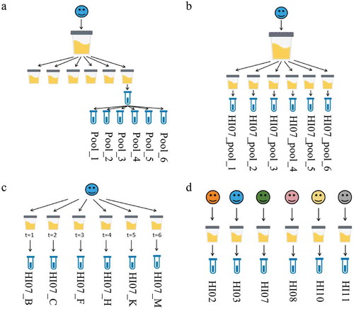
The total variation is represented by the interbiological, intrabiological, technical and instrumental variation. In order to determine these variation parameters, different experimental set-ups were used (Figure 1). To evaluate the instrumental variation, the same sample was analysed six times on the mass spectrometer (Pool_1 until Pool_6). This variation parameter was only determined for the proteomics analysis (Figure 1(a)). To evaluate the total technical variation (EV isolation method + MS sample preparation method + instrumental), six identical pooled urine samples of one individual (HI07_pool_1 until HI07_pool_6) were used as starting material for six EV isolations. EV samples were separately processed and loaded on the mass spectrometer (Figure 1(b)). To establish the intrabiological variation (also including the total technical variation), six urine samples of one individual (HI07_B/_C/_F/_H/_K/_M) at different time points were used (Figure 1(c)). The comparison of the urinary EV proteins and lipids of six different individuals (HI02/HI03/HI07/HI08/HI10/HI11) captures all the above variation and the interbiological variation, representing the total variation (Figure 1(d)).

Figure 1. Experimental set-ups of variation. The total variation is represented by: (a) the instrumental variation (b) the total technical variation (c) the intrabiological variation and (d) the interbiological variation. The names of the samples are indicated.

Protein and lipid identification and quantification

EVs were isolated from the urine samples by ultrafiltration (UF) in combination with size exclusion chromatography (SEC) [11]. Lipids and proteins of the EVs were separated by methyl-tert-butyl ether (MTBE) extraction [12,13]. In this way, variation parameters at protein as well as lipid level were determined using the same samples. EV protein concentration was determined using Micro BCA™ Protein Assay Reagent Kit (Thermo Scientific, Waltham, USA), and values between 0.18 and 0.50 µg per mL of starting volume urine for each sample were obtained.

Proteomic analysis

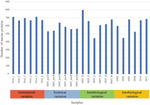
Shotgun proteomics (liquid chromatography-tandem mass spectrometry, LC-MS/MS) was performed on a Q-Exactive plus mass spectrometer (Thermo Fisher Scientific). For protein identification, the raw data were interpreted with both Sequest and Mascot as described in the method section. Between 1630 and 3318 peptides were identified with high confidence per sample. This results in 447 to 800 master proteins that were identified in each sample using Proteome Discoverer 2.1 with protein database Uniprot Human Proteome ID (UP000005640, downloaded on 25 May 2016). Figure 2 shows the number of master proteins identified in each sample. A list of all the 1518 identified master proteins using Proteome Discoverer 2.1 is shown in the supplementary data.

Figure 2. Number of master proteins per sample in each variation set-up. Samples Pool_1 until Pool_6 were used for the instrumental variation. The samples HI07_pool_1 until HI07_pool_6 were used to calculate the total technical variation. Samples HI07_B/_C/_F/_H/_K/_M were used to determine the intrabiological variation and HI02/HI03/HI07_M (further called HI07)/HI08/HI10/HI11 for the interbiological variation.

The raw data and identifications underwent a quality control analysis using an in-house developed software in R to check if all samples were correctly analysed and no problems occurred during sample handling or LC-MS/MS. For example, retention times of the same peptide in different samples and mass calibrations were checked. All samples passed the quality control analysis.

Differential proteomic analysis based on peptide identification (as is routinely done in shotgun proteomics) is hampered by its low analytical reproducibility since peptides are selected in a data-dependent way (data-dependent acquisition) and therefore, it cannot be guaranteed that the same set of peptides is identified across different LC-MS/MS runs. This is solved using an analytical workflow that extracts intensity chromatograms from high-resolution MS1 data to quantify all highly confident identified peptides across all samples. Several software packages (i.e. Skyline, MaxQuant, Progenesis QI) exist that automate this process of data enrichment [14–17]. We used an in-house developed data enrichment process that maximizes proper peak selection by using visual inspection and controlling tools like retention time curves, comparison of measured masses, etc. We only used peptides that are unique in the Uniprot Human Proteome ID (UP000005640, downloaded on 25 May 2016). After the extraction of reliable MS1 data, we were able to quantify 4926 peptides.

Lipidomic analysis

For the lipid identification, high-resolution LC coupled to high-resolution quadrupole time-of-flight MS was performed on an Agilent 6545 Q-TOF mass spectrometer (Agilent Technologies) [9,18]. A more detailed description of the lipidomic analysis, data processing and lipid identification is available in material and methods. A targeted data processing of the lipid profiles was performed based on an in-house accurate mass-retention time (AMRT) library [9]. All lipids identified in the vesicles are shown in the supplementary data.

Normalization and variance analysis

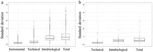
Median intensity normalization was applied on both proteomic and lipidomic data using R and is explained in the material and methods section [19]. The standard deviation (SD) of the normalized log intensities was determined. Figure 3 represents the percentage of unique peptides or lipids of the different variation set-ups in the function of the SD. This graph demonstrates that 90% of the least variable unique peptides of the total variation set-up do not have an SD that exceeds 2 (Figure 3(a)). For the 90% least variable lipids of the total variation set-up, this graph demonstrates that they do not have an SD that exceeds 1.2 (Figure 3(b)). These values can be used in the sample size calculation. Figure 4 shows the boxplots of the SD of the normalized log intensity of the different types of variation for both the proteomic and lipidomic data.

Figure 3. Percentage of unique peptides and lipids of the different variation set-ups in the function of the standard deviation (SD) of normalized log intensity. (a) 90% of the least variable peptides of the total variation set-up leads to an SD of 2. (b) The 90% least variable lipids of the total variation set-up do not have an SD that exceeds 1.2.

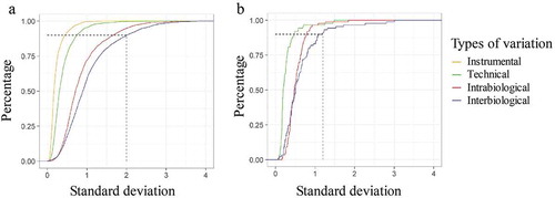
Figure 4. Boxplot of standard deviation (SD) of normalized log intensity of the different variation set-ups. (a) SD of the instrumental, technical, intrabiological and total variation is shown for the proteomic data. (b) SD of the technical, intrabiological and total variation is shown for the lipidomic data.

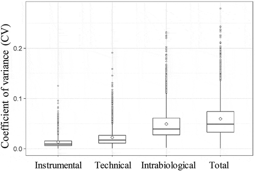
The coefficient of variation (CV) of the quantified peptides in the different proposed set-ups was also calculated, i.e. for each quantified peptide the SD of the intensities was divided by the mean of the intensities. This value also gives an indication about the variation, but normalizes the SD for the mean intensity. Figure 5 shows the boxplots of the CVs of the different types of variation. The mean CVs were 0.01, 0.02, 0.04 and 0.05 for the instrumental, technical, intrabiological and interbiological variation, respectively.

Figure 5. Boxplots of coefficients of variance (CVs) of the peptides in the different variation set-ups (instrumental, technical, intrabiological and total variation).

Sample size calculation

A sample size calculation is based on the following factors: the SD, a peptide fold change (after normalization) or effect size, type I error α and power. Table 1 shows the sample size needed in each group, given a power of 80% and α equal to 0.001. Depending on the effect size, the amount of samples needed in each group of the biomarker discovery experiment at EV level is shown.

Discussion

Urinary EVs are a suitable source of biomarkers for urological diseases including cancer, due to their origin, molecular content and function [20,21]. EV-based diagnostics could be a great alternative to invasive biopsies and cystoscopies [22]. The content of EVs can also give more insights into the relevant pathways of disease development to optimize personalized treatment and prognosis.

Variability in the urinary EV cargo caused by biological variation and technical variation due to sample preparation and instrumentation has an impact on the experimental study design as variation influences statistical power. To avoid false discoveries driven by underpowered quantitative discovery experiments, it is essential to determine the global variation in real samples. This is a first step in biomarker discoveries since a well-designed discovery study is very important. Reliable candidates are desired rather than false-positive biomarker candidates since validation procedures take a lot of time and money. Here, we described an analytical set-up that can be applied for the identification of variability arising from biological and technical variation in EV samples at the protein and lipid level.

Experimental set-ups of variation were used to determine the technical and biological variation. The SD of the unique peptides and lipids were determined in each experimental set-up. The technical variation of lipids in EVs is lower than the technical variation of peptides (0.5 versus 0.75). This is probably partly due to the targeted method used for the lipid identification and quantification. Here, only a certain set of lipids is quantified. For proteomics, a shotgun method is used for the identification and peptides are quantified using MS1 quantification. It is important to remark that if another protocol is used (EV isolation method, MS sample preparation, etc.) technical variability may be different. Also, the intrabiological variability of the lipids is lower than of the peptides (0.8 versus 1.7). This can be expected since the main function of the lipids in EVs is forming a lipid bilayer that provides the EVs structure and the potential to package signal molecules [23]. Proteins have a more complex communication and signalling function [18,24,25]. However, the lipid composition of the EVs also can have biological activity and in this way can be used as a biomarker [26–28]. Figure 3 shows that the 90% least variable peptides and lipids of the total variation set-up did not have an SD that exceeds 2 and 1.2, respectively. The lower technical and intrabiological variation of lipids is contributing to the lower total variation of lipids.

We started from healthy individuals, of which the age is related to a population that is expected to have more urological malignancies [9,10]. It needs to be further evaluated if the outcome for the healthy individuals is valid for patients too. Patients are expected to have more EVs and probably with a different cargo [29–31].

The sample size calculation gives a minimum of samples needed for a biomarker discovery. The question can be asked if studies using less samples are statistically relevant. Studies with a sufficiently large sample size are expected to be more relevant [32,33]. However, the number of samples needed is still dependent on a lot of factors. In this sample size calculation for the proteomics data, we took only one unique peptide per protein into account to calculate the number of samples needed in a differential protein biomarker discovery. If two or more unique peptides are identified per protein, this number of samples per group decreases to obtain statistically relevant differential protein biomarkers. Also, the effect size and power influence the sample size.

Nagaraj et al. (2011) determined the degree of normal urinary proteome variability of healthy individuals. The reported interbiological CV was 0.66, including the technical as well as the intrabiological variation. The intrabiological and technical CV was 0.48 and 0.18, respectively [34]. In our study, Figure 5 shows that the mean CVs of the EV proteins were lower (0.01, 0.02, 0.04 and 0.05 for the instrumental, technical, intrabiological and interbiological, respectively). This is expected since the variability of the urinary proteome is thought to be high because most of the proteins in the urine have no functional role anymore and there is no physiological need for precise homoeostatic control [34]. On the other hand, proteins in urinary EVs do have a functional role in physiological and pathophysiological conditions so are expected to be less variable [35–37].

Although less variation is expected in EVs than the urinary proteome since most of the proteins in the urine have no functional role anymore and there is no physiological need for precise homoeostatic control [34] and urinary EVs do have a functional role in physiological and pathophysiological conditions [35–37], variability is still high. The technical variability is already high for both peptides and lipids causing the need for an adequate number of technical replicates. The total variation at the EV level is also high. It should be mentioned that it is possible that not solely EV related proteins and lipids are taken into account in the variance analysis. Samples can be contaminated with urinary proteins and lipids. Also, cell disruption due to the freeze-thaw cycle of urine causes the presence of cell components in the cell-free urine. Isolated non-EV related proteins and lipids can have a higher variability. However, the EV isolation method UF in combination with SEC will enrich the EVs and remove most of the contaminants. A sample size calculation using these calculated variation parameters can be done for a differential biomarker discovery study at EV protein or lipid level.

Materials and methods

Urine collection

The human biological material (urine) used in this publication was provided by Biobank@UZA (Antwerp, Belgium; ID: BE71030031000); Belgian Virtual Tumorbank funded by the National Cancer Plan, BBMRI-ERIC [30]. Voided urine was obtained with written informed consent (approved by the Ethical Committee of the University of Antwerp and the University Hospital of Antwerp) from six healthy individuals (HI). Table 2 gives an overview of the sex and age of the individuals.

One urine sample of individuals HI02, HI03, HI08, HI10 and HI10 was collected. Six different samples of individual HI07 were obtained at different time points. All samples were collected using the urine vacuette system (Vacuette®, Greiner bio-one, Austria). The samples were stored immediately at −20°C. Based upon literature with some modifications [38], samples were thawed and centrifuged at 180 x g for 10 min at 4°C and at 1550 x g for 20 min at 4°C and pellets were discarded to prepare cell-free urine. Samples were subsequently stored at −80°C until further use.

EV isolation

EVs were isolated from the urine samples as described by [11]. Prior to the SEC isolation, ultrafiltration (UF) was performed to reduce the volume and remove smaller particles and proteins [39]. Per isolation procedure, 50 mL of cell-free urine was thawed and filtered using 100 kDa MWCO Centricon® Plus-70 Centrifugal Filter Units (Merck Millipore Ltd, Ireland) to get rid of the solute and small proteins.

The filtrate was placed on a qEV column (Izon Science Ltd, New Zealand). 500 µL fractions were collected, started immediately after placing the sample on the column, with filtered PBS as the elution buffer. The qEV columns are used according to the manufacturer’s instructions.

EV characterization of the isolated EVs was not performed since this EV isolation method was validated in our recent publication [11]. Transmission electron microscopy, western blotting, nanoparticle tracking analysis and asymmetrical-flow field-flow fractionation were used to validate the isolation method, demonstrating the enrichment of urinary EVs in the samples.

Protein concentration

Total protein content was determined using the Micro BCA™ Protein Assay Reagent Kit (Thermo Fisher Scientific, Waltham, USA) following the manufacturer’s specifications. A standard curve of serially diluted Bovine Serum Albumin (Thermo Fisher Scientific) in filtered PBS was used. Values were extrapolated from this curve, using a linear equation, with r² > 0.98 for each assay [40].

MTBE extraction

UF-SEC fractions in PBS were vacuum dried in 2 mL Eppendorf protein LoBind tubes to obtain a pellet of EVs. An MTBE lipid extraction method was applied to the samples, based on the procedure described by Matyash et al. [12,13]. The pellet was suspended in 300 µL methanol and vortexed for 10 s. 1 mL of MTBE (Sigma, Belgium) was added and samples were shaken for 1 h at room temperature. For the phase separation, 260 µL water was added. After 10 min of incubation at room temperature, samples were centrifuged for 10 min at 1000 x g, resulting in a lower hydrophilic and upper lipophilic phase. The first mL of the upper phase was removed, vacuum dried and further used for the lipidomic analysis. The lower hydrophilic and protein layer was vacuum dried and used in the proteomic analysis.

Proteomic analysis

In solution digest

The vacuum dried hydrophilic and protein layer were resuspended in 75 µL 5 M urea. Samples were vortexed and sonicated for 10 min. This step was repeated. Proteins were reduced in a final concentration of 5 mM dithiothreitol at 60°C for 30 min. Proteins were alkylated in a final concentration of 20 mM iodoacetamide in the dark at room temperature for 30 min. Subsequently, 680 µL 100 mM ammonium bicarbonate was added. For the digestion step, 1 µg trypsin was added per 40 µg of protein and digestion was carried overnight at 37°C. Digests were desalted using Pierce C18 spin columns (Thermo Fisher Scientific) according to manufacturer’s instructions.

LC-MS/MS

The purified peptides were vacuum dried and dissolved in mobile phase A, containing 2% acetonitrile and 0.1% formic acid to a final concentration of 1 µg/µL, and spiked with 20 fmol Glu-1-fibrinopeptide B (Glu-fib, Protea biosciences, Morgantown, WV). Samples were analysed in random order. A total of 2 µg of protein was loaded on the column and the peptide mixture was separated by reversed-phase chromatography using an nanoACQUITY UPLC Symmetry C18 Trap Column (100Å, 5 µm, 180 µm x 20 mm, 2G, V/M, 1/pkg) (Waters, Milford, MA) connected to an ACQUITY UPLC PST C18 nanoACQUITY Column (10K psi, 130Å, 1.7 µm, 100 µm X 100 mm, 1/pkg) (Waters). A linear gradient of mobile phase B (0.1% formic acid in 98% acetonitrile) from 1% to 45% in 95 min followed by a steep increase to 90% mobile phase B in 10 min. A steep decrease to 1% mobile phase B is achieved in 5 min and 1% mobile phase B is maintained for 5 min. The flow rate is 400 nL per minute. Liquid chromatography was followed by tandem MS (LC-MS/MS) and was performed on a Q-Exactive plus MS (Thermo Fisher Scientific). A nanospray ion source (Thermo Fisher Scientific) was used. Full-scan spectrum (350 to 1850 m/z, resolution 70,000, automatic gain control 3E6, maximum injection time 100 ms) was followed by high-energy collision-induced dissociation (HCD) tandem mass spectra with a run time of 90 min. Peptide ions were selected for fragmentation by tandem MS as the 10 most intense peaks of a full-scan mass spectrum. HCD scans were acquired in the Orbitrap (resolution 17,500, automatic gain control 1E5, maximum injection time 80 ms).

Peptide identification

Proteome Discoverer (2.1) software (Thermo Fisher Scientific) was used to perform database searching against the database containing Uniprot Human (Proteome ID: UP000005640, downloaded on 25 May 2016), using both Sequest and Mascot search engines. Searches were performed with the following settings: precursor mass tolerance of 10 ppm, fragment mass tolerance of 0.02 Da. Digestion by trypsin and two missed cleavage sites are allowed. Carbamidomethyl was defined as a fixed modification and phosphorylation (S, T, Y) and oxidation (of methionine) were dynamic modifications. The results were filtered with the following parameters: only high confident peptides with a global FDR < 1% based on a target-decoy approach and first ranked peptides were included in the results.

Quality control analysis

The MS/MS results (raw data) together with the Proteome Discoverer results were inspected in a quality control (QC) analysis. In our lab, QC analysis is done systematically as it guarantees the quality of the sample and the MS instruments at each moment for each sample. If for several reasons, samples do not meet the requested QC parameters, for example, reproducibility of retention time and mass calibration, these samples are excluded for further data analysis steps.

Data enrichment process

It is known that data-dependent acquisition (DDA) of mass spectrometry-based proteomics leads inherently to a lot of missing data points as not every peptide precursor measured in MS1 is selected for fragmentation and only the intensities of identified peptides are taken into account. To get quantitative data on all peptides for each sample, we developed in-house software to look up peak intensities in the raw MS1 data. In short, this software tool looks up m/z values in raw MS1 data with a delta ppm of 5 in a retention time window of 10 min. The quality control analysis guarantees that retention times are reproducible in all runs and mass calibration is correct. The algorithm also cleans the resulting data by using a decoy search and also peak shape is checked. That way, a data matrix is obtained containing quantitative information from almost all identified peptides. This in-house developed technique is similar and available in several software packages like MaxQuant, Skyline and Progenesis QI [14–17].

Lipidomic analysis

MS method

The LC-MS method was adapted from Sandra et al. [41]. The samples (10-µL injection volume) were chromatographically separated on an Acquity UPLC BEH Shield RP18 column (2.1 x 100 mm; 1.7 μm; Waters). Chromatographic separation was achieved on an Agilent 1290 Infinity LC system (Infinity Binary Pump G4220A, Thermostat G1330B, Infinity Sampler G4226A; Agilent Technologies). The column temperature was maintained at 80°C using a stand-alone Sandra/Selerity Series 9000 Polaratherm oven (Selerity Technologies, Salt Lake City, UT, USA). Eluting buffers were buffer A (20 mM ammonium formate, pH 5) and buffer B (MeOH). Starting conditions were 50% of buffer B at a flow rate of 0.5 mL/min. Over 5 min, a gradient was applied to 74% of buffer B. Thereafter the percentage of buffer B was increased to 100% in subsequent gradients (5–6 min 74–85% B; 6–16 min 85–90% B; 16–17 min 90–94% B; 17–26 min 94–100% B), before returning to the starting conditions (50% B) which was hold for 9 min.

High-resolution accurate mass spectra and fragmentation spectra were obtained with an Agilent 6545 Q-TOF MS instrument (Agilent Technologies) equipped with a Dual Jetstream electrospray ionization (ESI) source. The instrument was operated in positive electrospray ionization mode. Needle voltage was optimized to 3.5 kV, the drying and sheath gas temperatures were set to 300°C and 350°C and both drying and sheath gas flow rates were set to 8 L/min, respectively. Data were collected in centroid mode from m/z 100–1700 at an acquisition rate of 2 spectra/s in the extended dynamic range mode (2 GHz), offering an in-spectrum dynamic range of 10⁵ and a resolution of ± 20,000 FWHM in the lipid m/z range. To maintain mass accuracy during the analysis sequence, a reference mass solution was used containing reference ions (m/z 121.050873 and 922.009798 for positive ESI mode). Data acquisition was performed using MassHunter Acquisition B.06.01. Study samples were analysed in randomized order. Samples were kept at 4°C in the autosampler tray while waiting for injection.

Lipid identification

An in-house accurate mass retention time (AMRT) library with formula, exact mass and retention time of all identified lipids in comma-separated values (.csv) format (compatible with the MassHunter software) provided an automated and targeted data-processing of LC-MS lipid profiles [9]. Raw LC-MS data files were processed in a targeted fashion using the Find by Ion extraction algorithm in Profinder B08.00 (Agilent Technologies) using predefined mass (10 ppm) and retention time extraction windows (10 sec). The Agile integrator was used, with an absolute peak height cut-off of 1000 counts.

Lipid nomenclature

Throughout the manuscript, the nomenclature of the International Lipid Classification and Nomenclature Committee (ILCNC) has been used, i.e. ‘‘Comprehensive Classification System for Lipids”. 32–34 Lipids for which the exact structure of the two acyl chains could not be elucidated are listed with the total number of carbon atoms and double bonds of the fatty acyl moiety, e.g. phosphatidyl inositol (PI) (34:2). The aliphatic chain composition and region-specificity of these compounds can be identified with further MS/MS analyses. Regarding glycosphingolipids, LC-MS cannot discriminate between galactose and glucose or N-acetylglucosamine and N-acetylgalactosamine. Therefore, lipid nomenclature of these species contains hexose (Hex) instead of glucose or galactose.

Statistical analysis

Statistical analysis was done in R using standard R-core and Bioconductor packages [42,43]. The packages Normalizer was used for normalization [19]. Median intensity log normalization was used on the intensity of the proteomic and lipidomic data: Here, the intensity of each variable in a given sample is divided by the median of intensities of all variables in the sample and multiplied by the mean of “median of sum of intensities of all variables in all samples”. The normalized data is then transformed to log2. After determining the SD of peptides, a sample size calculation was done in R based on a simple t-test in order to calculate a minimum sample size needed for a valid two-group experimental design.

EV-TRACK

We have submitted all relevant data of our experiments to the EV-TRACK knowledgebase (EV-TRACK ID: EV190004) (Van Deun J, et al. EV-TRACK: transparent reporting and centralizing knowledge in extracellular vesicle research. Nature methods. 2017;14(3):228–32) [44]. The EV-METRIC score was 63%. For the characterization, we refer to our previous paper where the EV isolation method used in this study is described extensively.

Disclosure of Interest

The authors report no conflict of interest.

Acknowledgments

We are grateful to the Flemish Institute for Technological Research for the support and funding of this research.

Additional information

Funding

This work was supported by the Vlaamse Instelling voor Technologisch Onderzoek.

References

- Al-Nedawi K. The yin-yang of microvesicles (exosomes) in cancer biology. Front Oncol. 2014;4:172.
- Corrado C, Raimondo S, Saieva L, et al. Exosome-mediated crosstalk between chronic myelogenous leukemia cells and human bone marrow stromal cells triggers an interleukin 8-dependent survival of leukemia cells. Cancer Lett. 2014;348(1–2):71–10.
- Spanu S, van Roeyen CRC, Denecke B, et al. Urinary exosomes: a novel means to non-invasively assess changes in renal gene and protein expression. PLoS One. 2014;9(10):e109631.
- Barros ER, Carvajal CA. Urinary exosomes and their cargo: potential biomarkers for mineralocorticoid arterial hypertension? Front Endocrinol. 2017;8:230.
- Nawaz M, Camussi G, Valadi H, et al. The emerging role of extracellular vesicles as biomarkers for urogenital cancers. Nat Rev Urol. 2014;11(12):688–701.
- Zhou H, Yuen PST, Pisitkun T, et al. Collection, storage, preservation, and normalization of human urinary exosomes for biomarker discovery. Kidney Int. 2006;69(8):1471–1476.
- Maes E, Valkenborg D, Baggerman G, et al. Determination of variation parameters as a crucial step in designing TMT-based clinical proteomics experiments. PLoS One. 2015;10(3):e0120115.
- Cairns DA. Statistical issues in quality control of proteomic analyses: good experimental design and planning. Proteomics. 2011;11(6):1037–1048.
- Batista-Miranda JE, Molinuevo B, Pardo Y. Impact of lower urinary tract symptoms on quality of life using functional assessment cancer therapy scale. Urology. 2007;69(2):285–288.
- Lawhorne LW, Ouslander JG, Parmelee PA, et al. Urinary incontinence: a neglected geriatric syndrome in nursing facilities. J Am Med Dir Assoc. 2008;9(1):29–35.
- Oeyen E, Van Mol K, Baggerman G, et al. Ultrafiltration and size exclusion chromatography combined with asymmetrical-flow field-flow fractionation for the isolation and characterisation of extracellular vesicles from urine. J Extracell Vesicles. 2018;7(1):1490143.
- t’Kindt R, Telenga ED, Jorge L, et al. Profiling over 1500 lipids in induced lung sputum and the implications in studying lung diseases. Anal Chem. 2015;87(9):4957–4964.
- Matyash V, Liebisch G, Kurzchalia TVet al. Lipid extraction by methyl-tert-butyl ether for high-throughput lipidomics. J Lipid Res. 2008;49(5):1137–1146.
- Cox J, Mann M. MaxQuant enables high peptide identification rates, individualized p.p.b.-range mass accuracies and proteome-wide protein quantification. Nat Biotechnol. 2008;26(12):1367–1372.
- Tyanova S, Temu T, Cox J. The MaxQuant computational platform for mass spectrometry-based shotgun proteomics. Nat Protoc. 2016;11(12):2301–2319.
- MacLean B, Tomazela DM, Shulman N, et al. Skyline: an open source document editor for creating and analyzing targeted proteomics experiments. Bioinformatics. 2010;26(7):966–968.
- Megger DA, Bracht T, Meyer HE, et al. Label-free quantification in clinical proteomics. Biochim Biophys Acta. 2013;1834(8):1581–1590.
- Thery C, Ostrowski M, Segura E. Membrane vesicles as conveyors of immune responses. Nat Rev Immunol. 2009;9(8):581–593.
- Chawade A, Alexandersson E, Levander F. Normalyzer: a tool for rapid evaluation of normalization methods for omics data sets. J Proteome Res. 2014;13(6):3114–3120.
- Sun Y, Liu J. Potential of cancer cell-derived exosomes in clinical application: a review of recent research advances. Clin Ther. 2014;36(6):863–872.
- Hoorn EJ, Pisitkun T, Zietse R, et al. Prospects for urinary proteomics: exosomes as a source of urinary biomarkers. Nephrology (Carlton). 2005;10(3):283–290.
- Jia S, Zocco D, Samuels ML, et al. Emerging technologies in extracellular vesicle-based molecular diagnostics. Expert Rev Mol Diagn. 2014;14(3):307–321.
- Trajkovic K, Hsu C, Chiantia S, et al. Ceramide triggers budding of exosome vesicles into multivesicular endosomes. Science. 2008;319(5867):1244–1247.
- Marimpietri D, Petretto A, Raffaghello L, et al. Proteome profiling of neuroblastoma-derived exosomes reveal the expression of proteins potentially involved in tumor progression. PLoS One. 2013;8(9):e75054.
- Hosseini-Beheshti E, Pham S, Adomat H, et al. Exosomes as biomarker enriched microvesicles: characterization of exosomal proteins derived from a panel of prostate cell lines with distinct AR phenotypes. Mol Cell Proteomics. 2012;11(10):863–885.
- Kim CW, Lee HM, Lee TH, et al. Extracellular membrane vesicles from tumor cells promote angiogenesis via sphingomyelin. Cancer Res. 2002;62(21):6312–6317.
- Del Boccio P, Raimondo F, Pieragostino D, et al. A hyphenated microLC-Q-TOF-MS platform for exosomal lipidomics investigations: application to RCC urinary exosomes. Electrophoresis. 2012;33(4):689–696.
- Choi DS, Lee J, Go G, et al. Circulating extracellular vesicles in cancer diagnosis and monitoring: an appraisal of clinical potential. Mol Diagn Ther. 2013;17(5):265–271.
- Taylor DD, Gercel-Taylor C. MicroRNA signatures of tumor-derived exosomes as diagnostic biomarkers of ovarian cancer. Gynecol Oncol. 2008;110(1):13–21.
- Liang LG, Kong M-Q, Zhou S, et al. An integrated double-filtration microfluidic device for isolation, enrichment and quantification of urinary extracellular vesicles for detection of bladder cancer. Sci Rep. 2017;7:46224.
- Oeyen E, Hoekx L, De Wachter S, et al. Bladder cancer diagnosis and follow-up: the current status and possible role of extracellular vesicles. Int J Mol Sci. 2019;20(4).
- Lin SY, Lin Z, Buawangpong N, et al. Proteome profiling of urinary exosomes identifies alpha 1-antitrypsin and H2B1K as diagnostic and prognostic biomarkers for urothelial carcinoma. Sci Rep. 2016;6:34446.
- Long JD, Sullivan TB, Humphrey J, et al. A non-invasive miRNA based assay to detect bladder cancer in cell-free urine. Am J Transl Res. 2015;7(11):2500–2509.
- Nagaraj N, Mann M. Quantitative analysis of the intra- and inter-individual variability of the normal urinary proteome. J Proteome Res. 2011;10(2):637–645.
- Yanez-Mo M, Siljander PR, Andreu Z, et al. Biological properties of extracellular vesicles and their physiological functions. J Extracell Vesicles. 2015;4:27066.
- Filipazzi P, Bürdek M, Villa A, et al. Recent advances on the role of tumor exosomes in immunosuppression and disease progression. Semin Cancer Biol. 2012;22(4):342–349.
- Franzen CA, Blackwell RH, Todorovic V, et al. Urothelial cells undergo epithelial-to-mesenchymal transition after exposure to muscle invasive bladder cancer exosomes. Oncogenesis. 2015;4:e163.
- Yuana Y, Böing AN, Grootemaat AE, et al. Handling and storage of human body fluids for analysis of extracellular vesicles. J Extracell Vesicles. 2015;4:29260.
- Abramowicz A, Widlak P, Pietrowska M. Proteomic analysis of exosomal cargo: the challenge of high purity vesicle isolation. Mol Biosyst. 2016;12(5):1407–1419.
- Webber J, Clayton A. How pure are your vesicles? J Extracell Vesicles. 2013;2:19861.
- Sandra K, Pereira ADS, Vanhoenacker G, et al. Comprehensive blood plasma lipidomics by liquid chromatography/quadrupole time-of-flight mass spectrometry. J Chromatogr A. 2010;1217(25):4087–4099.
- Team, R.C. R: a language and environment for statistical computing. R foundation for statistical computing. 2018. Available from: https://www.R-project.org/
- Gentleman RC, Carey VJ, Bates DM, et al. Bioconductor: open software development for computational biology and bioinformatics. Genome Biol. 2004;5(10):R80.
- Consortium E-T, Van Deun J, Mestdagh P, et al. EV-TRACK: transparent reporting and centralizing knowledge in extracellular vesicle research. Nat Methods. 2017;14(3):228–232.