Effect of financial sector development and institutions on economic growth in SSA. Does the peculiarities of regional blocs matter?

ABSTRACT

The link between financial sector development (FSD) and economic growth has generated a great deal of interest among academics. Some studies argued that financial sector stimulates growth while others suggested the opposite. Thus, we conducted a comparative analysis of the effect of FSD on economic growth between Economic Community of West African States (ECOWAS) and Southern African Development Community (SADC). In addition, we sought to find out the transmission of FSD through institutional development on economic growth. The results suggested the existence of FSD-led growth in SADC but revealed no statistically significant effect in ECOWAS. Furthermore, the effect of FSD through institutional development supported a positive complementarity effects on growth in both regions but only statistically significant in ECOWAS, suggesting strong institutions complemented FSD effects on growth. We recommended that ECOWAS take steps to improve both political structures and democratic dispensation to boost the development of the financial sector.

KEYWORDS:

• ECOWAS
• SADC
• financial development
• panel cointegration
• dynamic pooled

JEL CLASSIFICATION NUMBERS:

• G21
• O16
• O43
• O55

1. Introduction

Since the nineteenth century, financial sector development (FSD) has been identified as a key determinant of economic growth. For instance, the financial sector played a crucial role in facilitating the mobilization of capital for industrialization in England (Bagehot 1873) and assisted in channeling funds to productive investments (Schumpeter 1932) which constituted important determinants of economic growth. On the other hand, Patrick (1966) and Goldsmith (1969) argued that economic growth stimulates FDS to provide financial resources to the expanding sectors of the economy. Due to these conflicting outcomes, several empirical studies have tried to address the potential link between FSD and growth (see Akinboade and Makina 2006; Abu-Bader and Abu- Qarn 2008; Gazdar and Cherif 2015; Puatwoe and Piabuo 2019; Khan et al. 2019). In addition, prior studies have identified institutions as an important transmitting channel in stimulating economic growth among countries (Hall and Jones 1999; Acemoglu, Johnson, and Robinson 2001). Components of institutions such as democratic dispensation, competent bureaucracies, property rights protection, competent and incorruptible judiciary promote free movement of resources for economic growth.

Even though a good number of prior studies on FSD and economic growth have been conducted in SSA, they are either single-country/cross-country analysis or analysis of single bloc, neglecting an important investigation of comparative study of regional groupings in Sub-Saharan Africa (SSA) (see Atindéhou, Gueyie, and Amenounve 2005; Aboudou 2009; Loesse 2010; Fawowe 2011; Khan et al. 2019; Sabir et al. 2019). In response to the identified gaps, this study attempts to conduct a comparative analysis of the effect of FSD on economic growth between two economic-blocs: Economic Community of West African States (ECOWAS) and Southern African Development Community (SADC) in sub-Sahara Africa (SSA). Second, we estimate the effect of FSD through institutional development on economic growth in the two economic-blocs. By this, we will reveal the peculiarities in each bloc and the desired macroeconomic policy required to stimulate growth and also uncover the dynamic effect of FSD on economic growth. Again, these blocs are an important feature of international trade and represent about two-thirds of SSA’s population. Hence, a comparative study will reveal the deficiencies in each bloc and how to promote integration and development. Third and finally, we employ the latest advances in panel approaches and account for time series properties of the variables which are often ignored in earlier studies leading to inefficient results.

The remainder of this study is structured as follows. Section 2 discusses the background of SADC and ECOWAS. Section 3 provides both theoretical and empirical literature on FSD and growth. Section 4 discusses the model and econometric technique and data used. Section 5 presents discussion of results while Section 6 presents the conclusion.

2. Background and characteristics of ECOWAS and SADC

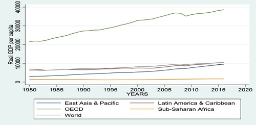
Africa is one of the least developed continents in the world. The continent accounts for 28% of the world’s poverty, 1% of global GDP, 2% of global trade and 3% of foreign direct investment (World Bank 2009; UNCTAD 2009). For instance, SSA’s real per capita income falls below the world’s trends as revealed in Figure 1. In 1980s, the per capita income of Latin America and Caribbean was about US$2000 higher than that of East Asia and Pacific but this difference was eliminated by 2009. However, SSA had a per capita income of about US$900 and by 2010 it rose negligibly to about US$1000 and US$1600 in 2016.

Figure 1. Comparison of real GDP per capita between SSA and other regions. Source of data: World Development Indicators (2016).

For over a decade, African countries have formed regional groupings to stimulate trade and economic cooperation, raise growth rate and reduce poverty. Other groupings include East African Community, Community of Sahel-Saharan States, Economic Community of Central African States and Intergovernmental Authority on Development. Sub-groups include Common Monetary Agreement (CMA), West Africa Monetary Union (WAMU), Economic and Monetary Community of Central Africa, Southern Africa Custom Union (SACU). Studies on the link between FSD and growth in regional blocs in SSA reveal mixed results. Atindéhou, Gueyie, and Amenounve (2005) on ECOWAS showed weak causal link and Aboudou (2009) reveals finance leads growth in WAMU. However, a comparative study of these regional blocs which is an integral part of development has been ignored.

Regarding FSD, credit to the private sector as a percentage of GDP and credit by the banking sector as a percentage of GDP for the period 1990–2016 for SADC did not only fall below SSA standards but also other developing economies of Latin America and Caribbean and East Asia and Pacific as reported in Table 1. However, South Africa performs more than twice the SSA average, followed by Mauritius. The story is the same considering financial sector depth with M2 as a percentage of GDP.¹ ECOWAS financial sector is dominated by banks. Table 2 reports that average private sector credit as a percentage of GDP (14%) is low compared to that of SSA (50%). However, those of Cape Verdi, Cote D’voire, Mali, Senegal and Togo are above ECOWAS' average. Guinea performs poorly during this period with 5.16% economic activities as credit to the private sector. Banking sector credit as a percentage of GDP is 32.92% and this shows that average financial sector activity is less than half of economic activity of the bloc. However, it is about 38% of GDP for Cape Verdi and 180% in Liberia.

Table 1. Financial sector development of member states of SADC.

Country/Region	Average credit to private sector (% of GDP)-1990–2016	Average credit by the banking sector as % of GDP-1990–2016	Average bank assets to bank assets and central bank assets (%) 1990–2016	M2% GDP-1990–2016	Interest rate Spread (1990–2016)
Angola	9.92	9.78	64.26	29.33	38.07
Bostwana	20.24	20.20	99.20	36.57	5.26
DRC	2.46	7.40	45.36	8.70	33.65
Lesotho	14.22	14.06	81.58	31.68	8.18
Madagascar	11.13	11.10	67.44	21.35	21.80
Malawi	9.27	8.25	62.79	37.25	18.81
Mauritius	67.04	67.01	97.78	86.89	7.16
Mozambique	14.76	14.66	87.43	26.73	8.97
Namibia	44.00	43.06	96.85	42.90	6.31
Seychelles	18.52	18.51	79.44	72.62	7.11
South Africa	129.06	64.78	97.65	62.52	4.11
Swaziland	17.08	16.96	98.15	22.21	6.66
Tanzania	9.38	9.21	74.63	20.59	11.55
Zambia	9.51	8.40	46.05	18.38	13.66
Zimbabwe	26.93	21.64	67.30	30.50	197.04
SADC	26.90	20.56	66.83	35.32	14.14
SSA	50.66	72.03	–	39.79	10.83
Latin America and Caribbean	36.16	33.70	–	42.58	7.54
East Asia and Pacific	143.79	121.43	–	167.38	4.62

Source of data: World Development Indicators (2016). Ratio of Bank assets to bank assets plus central bank asset is obtained from Global Financial Development Data base (2013).

Table 2. Financial sector development of member states of ECOWAS.

Country/Region	Average credit to private sector (% of GDP)-1990–2016	Average credit by the banking sector as a % of GDP-1990–2016	Average bank assets to bank assets and central bank assets (%) 1990–2016	M2% GDP-1990–2016	Interest rate Spread (2000–2016)
Benin	14.37	14.31	84.03	28.33
Burkina Faso	15.05	14.97	79.81	24.62	9.28
Cape Verdi	41.83	38.46	69.52	14.55	7.58
Cote D'voire	19.45	19.27	79.37	27.56	5.93
Gambia	7.41	16.20	79.68	22.38	14.01
Ghana	11.31	26.12	48.06	25.54	3.36
Guinea	5.14	15.30	30.02	26.01	13.18
Guinea Bissau	7.77	12.48	45.50	27.42
Liberia	8.18	180.61	11.52	14.76	12.26
Mali	15.43	14.28	79.45	22.57
Niger	8.81	10.79	62.17	15.89
Nigeria	8.81	21.99	63.80	16.51	7.49
Senegal	17.76	25.36	76.56	22.47
Sierra Leone	4.09	31.93	33.46	16.18	12.83
Togo	22.20	23.45	77.28	32.61
ECOWAS	13.99	32.92	61.35	25.49
SSA	50.66	72.03	–	39.79	10.83
Latin America and Caribbean	36.16	33.70	–	42.58	7.54
East Asia and Pacific	143.79	121.43	–	176.38	4.62

Source of data: World Development Indicators (2016) and Global Financial Development Database (2013).

The interest rate spread for six countries in SADC is below SSA level of 10.83%. However, interest rate spread of Zimbabwe is 197.04% which reflects the impact of the inflationary trends in that country. Other countries with higher interest rate spread include Angola, DRC, Madagascar and Malawi which is due to high bank concentration. In ECOWAS, the average depth of financial system is 23.62% with member states revealing less than 40% of economic activities, with only Ghana performing relatively better. Interest rate spread shows relative efficiency in the region with Ghana being competitive in the bloc while Gambia has the highest interest rate spread of 14.01%.

SADC has seven stock exchanges which are among the best in Africa. South Africa has the most developed stock market which ranks 17th in market capitalization globally. Table 3 reports that average stock market capitalization of listed companies is about 173% of economic activity in South Africa with market capitalization of US$362.096 billion for the period 1990–2011. Namibia performs the least with almost 8% of GDP and average total market capitalization of the period to be US$473.15 million. Zimbabwe and Mauritius (39.9%) operated less than 40% of GDP.

Table 3. Stock market development in SADC and ECOWAS.

Country/Region	Market capitalization of listed companies (% of GDP) 1990–2012	Market capitalization of listed companies (current US$)	Stocks traded, total value (current US$) 1990–2012	Stocks traded, total value (% of GDP) 1990–2012
Cote D'voire	15.72	2846844822	66131927.31	0.36
Ghana	13.25	1648130658	49653656.6	0.44
Nigeria	14.467	18730680701	2816223528	1.72
Botswana	21.29	2003545962	65013146.9	0.81
Mauritius	39.90	2686109803	156972959.4	2.27
Namibia	7.71	473152110.9	15949300.33	0.32
South Africa	172.46	362,096,000,000	1.5093E+11	61.22
Swaziland	9.924	184922748.8	–	–
Zambia	12.47	1241436503	44412232.13	0.43
Zimbabwe	87.33	5906300920	658688176.7	9.52
SSA	107.31	–	–	–
SSA	24.66	–	–	–

Source of data: GFDD (2013).

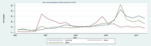
ECOWAS has three active stock markets namely: the Ghana Stock Exchange, Nigeria Stock Exchange and the Bourse Regionale des Valeurs Mobilieres (Abidjan) which serves WAMU member states. In Table 3, the average stock market capitalization of listed companies as a percentage of GDP was 15.72 for Bourse Regionale des Valeurs Mobilieres (BRVM) the highest for the bloc, followed by Nigeria Stock Exchange (14.5%) and then Ghana Stock Exchange (13.3%). However, Figure 2 reports improvements as these markets started from less than 10% in 1990 and grew steadily to 15% for Ghana, 14% for Cote D’voire and 17% for Nigeria by 2005. By 2007, the markets of Cote D’voire and Nigeria experienced an all-time high performance of 42% and 52% respectively. However, there was a sharp decline in performance in 2008 and 2009 due to debilitating effects of the financial turmoil of the period.

Figure 2. Stock market developments of the three Stock Exchange Markets in ECOWAS. Source of data: GFDD (2013).

In terms of total stock market capitalization, Nigeria recorded the highest average of 18.7307 billion current US$ during this period with Cote D’voire, 2.8468 billion current US dollars and Ghana, 1.6481 billion current US$ (see Table 3).

Even though the discussions suggest both blocs have relatively underdeveloped financial sectors, SADC seems to perform better than ECOWAS. Hence, comparative study relating finance to economic growth has implication for policy directions.

3. Literature review

King and Levine (1993) and Pagano (1993) suggest that higher financial development drives economic growth. Furthermore, new growth theory argues that financial markets and institutions are endogenous in response to market failures which contributes to economic growth. Levine (1997, 2005) reinforces that financial system causes economic growth through five channels: mobilizing savings, facilitating risk amelioration, acquisition of information on investment and allocating resources, monitoring managers and exerting corporate control and facilitating exchange of goods and services.

However, there are disagreements about the direction of causality. In one hand, some studies argue that causality runs from finance to growth (supply-leading hypothesis). On the other, Patrick (1966), Gurley and Shaw (1967) and Goldsmith (1969) argue that causation runs from growth to finance (demand-following). The third group argues that causation is bidirectional. Others such as McKinnon (1993) and Shaw (1973) indicate that constraints exerted by governments on the financial system can slow FSD, leading to low investments. Roubini and Sala-i-Martin (1995) also argue that financial repression does not only reduce output but also lowers savings which impedes economic growth and development.

The empirical literature shows diverse results. Wang (2000) shows that supply-leading is highly related to financial variables whereas demand-following is related to real variables that affect industrial production for Taiwan. Beck (2002) reveals a significant link between financial development on real per capita GDP growth and total factor productivity of 63 countries. On the contrary, Shan, Morris, and Sun (2001) use nine OECD countries including China and report a bidirectional causality among five countries. Deidda and Fattouh (2002) on the other hand find no significant relationship between financial depth and economic growth in low-income countries but the opposite holds for high income countries.

In Africa, Puatwoe and Piabuo (2019) estimate the effect of financial development on economic growth in Cameroun and find significant effect of FSD on economic growth. Odhiambo (2007) shows that causality between FSD and economic growth is sensitive to the proxy for financial development in South Africa, Tanzania and Kenya while Abu-Bader and Abu- Qarn (2008) reveal that FSD and economic growth are mutually causal. But Trabelsi (2002) finds that FSD affects growth only with cross-sectional estimates while Ghirmay (2004) reveals mixed result in finance–growth nexus. Khan et al. (2019) find that financial development through institutional quality affects economic growth in emerging countries and Gazdar and Cherif (2015) conclude that the quality of institutions moderates the adverse effect of financial development on growth. Similarly, Sabir et al. (2019) find positive effect of quality of institutions, financial development and technology on the growth of developing countries. Finally, Lida, Zahra, and Shahryar (2019) constructed an index and find that financial development adversely affects economic growth.

The empirical literature reveals the following. First, most of the extant studies used single variables to proxy FSD. However, Levine (1997) indicates that FSD is an improvement in the quality of five key financial functions including: (i) producing information on investment and allocating capital, (ii) monitoring and exerting corporate governance, (iii) facilitating trade and management of risk, (iv) mobilizing and pooling of risk and (v) easing exchange of goods and service. Thus, a single indicator cannot adequately measure financial development. Therefore, we construct a composite FSD index that includes three variables. Second, there exists no comparative study on the effects of FSD on growth on regional blocs of SSA. Regional blocs have become important and dominant feature of international trade but their comparison has been ignored in SSA. It is insightful to compare regional groups in SSA, since each bloc pursues similar policy goals towards meeting the convergence criteria set by the bloc (Mahawiya, Haim, and Oteng-Abayie 2020). We fill this gap by conducting a comparative analysis of FSD on growth for two regional groupings: ECOWAS and SADC. Finally, institutions that are expected to influence finance on growth also seems to be ignored in the studies of SSA. Thus, the effect of institutions in the form of democratic structures and dispensation on finance is captured in this study.

4. The model and econometric technique

Following the literature, we postulate a static panel model in a semi-log form: (1) $ln{y}_{t,i}=\alpha +{\text{β}}_{i}lnfinde{x}_{i,t}+{\gamma }_{i}ln{x}_{i,t}+{\phi }_{i}in{s}_{i,t}+{ϵ}_{i,t}$(1) where i is the individual country at time t and i = 1, … , N, t = 1, … , T, $ln{y}_{t,i}$ is the log of real GDP per capita and $lnfinde{x}_{i,t}$ measures log of FSD, $ln{x}_{i,t}$ is the log of control variables which includes openness, inflation, government expenditure and $in{s}_{i,t}$ represents polity 2 as institutional variable whereas ${ϵ}_{i,t}$ is the error term. Institutions and inflation are not logged because they are either negative or positive values. Following Allen et al. (2009), we differentiate Equation (1) to obtain a dynamic equation in (2). (2) $ln{y}_{growthi,t}=\alpha +{\text{β}}_i\mathrm{\Delta }lnfinde{x}_{i,t}+{\gamma }_i\mathrm{\Delta }ln{x}_{i,t}+{\phi }_{i}in{s}_{i,t}+{ϵ}_i$(2) Following the neo-classical growth model, we allow the initial real GDP per capita be log $y_{i,o}$ and steady-state real GDP per capita as $y_i^{\ast }.$ The first-order approximation implies $growt{h}_{i,t}=-\tau (y_{i,t}-$ $y_{i,t}^{\ast }$) where $\tau$ is the convergent parameter. Our final growth model is (3) $ln{y}_{growth}=\alpha -\tau ln{y}_{i,o}+{\text{β}}_i\mathrm{\Delta }lnfinde{x}_{i,t}+{\gamma }_i\mathrm{\Delta }ln{x}_{i,t}+{\phi }_{i}in{s}_{i,t}+{ϵ}_{i,t}$(3) For conditional growth convergence to occur, the coefficient of the initial real GDP per capita should be negative. The control variables openness and government expenditure are measured as a share of GDP. Theoretically, there is a positive relationship between growth and human capital which is controlled by the level of schooling. Unfortunately, there is no consistent data for this variable for the two subregions, so we dropped it.

We measure trade openness as the ratio of the sum of exports and imports to GDP. Exports could exert positive impact on growth if it results in increase in foreign exchange reserves and exchange of ideas and specialization. Imports can also propel growth if they are mainly capital goods and importation of foreign technology otherwise the effect could be negative. Therefore, net effect can be observed through empirical analysis. Government expenditure defines macroeconomic stability. Barro and Sala-i-Martin (1995) contended that government expenditure is productive when it goes into education, infrastructure and other activities that promote growth otherwise, it possesses a crowding-out effect which impairs growth. The theoretical expectation of inflation is negative. However, recent studies suggest nonlinearity and thresholds in inflation–growth relationship (Rousseau and Wachtel 2000; Seleteng, Bittencourt, and van Eyden 2013). These studies suggest that statistically significant effect is only noticeable at a certain threshold. Improved institutional environment affects growth positively (Acemoglu, Johnson, and Robinson 2004). We proxy $ins{t}_{i,t}$ with measures of political environment. Polity 2 describes the level of autocracy and democracy by assigning negative values to the former and positive for the latter. It ranges from –10 to +10, indicating total autocracy to total democracy respectively. Autocratic regimes are usually characterised by expropriation, bureaucracy, corruption and nepotism which may increase the cost of doing business and uncertainty about property rights. We expect a more autocratic regime to impair economic growth whereas more democratic regimes to facilitate the process of economic growth. In addition, it is contended that finance may influence economic growth through an efficient institutional environment. Hence, we include an interaction term between institution and finance in the estimated model. (4) $ln{y}_{{growth}_{i,t}}=\alpha -\tau ln{y}_{i,o}+{\text{β}}_i\mathrm{\Delta }lnfinde{x}_{i,t}+{\gamma }_i\mathrm{\Delta }ln{x}_{i,t}+{\phi }_{i}in{s}_{i,t}+{\omega }_i\mathrm{\Delta }\left(finde{x}_{i,t}\ast in{s}_{i,t}\right)+{ϵ}_{i,t}$(4) We measure $finde{x}_{i,t}$ by (5) ${\displaystyle \frac{1}{n}\sum _{j=1}^n\left[100\ast \left({\displaystyle \frac{F_{j,it}}{\overline{F}}}\right)\right]}$(5) where $F_j$ and $\overline{F}$ are FSD indicator and sample mean of $F_j$ respectively, n is the number of financial indicators used in the study. Equation (5) is estimated following Demirgüç-Kunt and Levine (1996). We include three FSD proxies: ratio of bank private credit to GDP, ratio of liquid liabilities (M3) to GDP and ratio of deposit money bank assets to the sum of deposit money bank assets and central bank assets. The bank private credit to GDP is a measure of size and isolate credit to the private sector by commercial bank excluding credit to government (Levine, Loayza, and Bech 2000). The ratio of deposit money bank assets to deposit money bank assets plus central bank assets (%) shows the influence of commercial banking sector in the economy. The ratio M3/GDP which proxies for financial depth is the sum of currency and deposits in the central bank (M0), plus transferable deposits and electronic currency (M1), plus time and savings deposits, foreign currency transferable deposits, certificates of deposit, and securities repurchase agreements (M2), plus travellers’ cheques, foreign currency time deposits, commercial paper, and shares of mutual funds held by residents. This proxy is preferred to M2 because M2 reflects more monetization rather than an increase in bank deposits (Eita and Jordaan 2007).

4.1. Panel unit root test

The use of long panel data series requires checking the stationarity of the series. A non-stationary time series do not revert to its long-run mean following a shock. We used Im, Pesaran, and Shin (2003) (IPS) and Levin, Lin, and Chu (2002) (LLC) to test the time series properties of the series based on the following AR (1) specifications: (6) $\mathrm{\Delta }{y}_{it}={\delta }_i+{\lambda }_{i}t+{\rho }_i{y}_{it-1}+{\mu }_{it}$(6) where t is the time trend, ${\delta }_i$ is the country-specific fixed effects, μ is the error term and ${\rho }_i$ is the autoregressive coefficient. If $\left|{\rho }_i\right|$ = 1, there is unit root in $y_{it}.$ LLC test assumes parameter homogeneity $({\rho }_i=\rho )$ and hence suffers from homogeneity bias whiles IPS allows for individual unit root processes. The null hypothesis for both tests states that there is the presence of unit root in all the series. However, the alternative differs. The alternative for LLC states there is stationarity in all variables but that of IPS states there is unit root in some of the series.

If non-stationary series are differenced to obtain I(1), then there could be the possibility of cointegration. Cointegrated variables require application of Granger (1988) causality tests through error correction model (ECM). The ECM includes lagged error correction term obtained from the cointegration equation into vector autoregression (VAR) to bring in information on long-run relationship that is wiped out as a result of the differencing. However, if the variables are I(1) but no cointegration, causal relationship can be estimated using VAR by eliminating the lagged error correction term.

We test for cointegration following Westerlund (2007) which assumes the error-correction tests follows data-generating process expressed as (7) $\mathrm{\Delta }{y}_{it}={\delta }_i{d}_t+{\alpha }_i\left(y_{i,t-1}-{\text{β}}_i^{\mathrm{\prime }}{x}_{i,t-1}\right)+\sum _{j=1}^{p_i}{\alpha }_{ij}\mathrm{\Delta }{y}_{i,t-j}+\sum _{j=1}^{p_i}{\gamma }_{ij}\mathrm{\Delta }{x}_{i,t-j}+e_{it}$(7) where t = 1, … , T and i = 1, … , N are indices of the time-series and cross-sectional units, respectively, and $d_t$ is the deterministic components. Westerlund (2007) tests models of K-dimensional vector $x_{it}$ as a pure random walk such that $x_{it}$ is independent of $e_{i{t}^{\mathrm{\prime }}}$ and further assumes that these errors are independent across both i and t. $y_{it}$ is real GDP per capita growth whereas $x_{it}$ refers to the regressors. Equation (7) can also be written as (8) $\mathrm{\Delta }{y}_{it}={\delta }_i{d}_t+{\alpha }_i{y}_{i,t-1}-{\theta }_i^{\mathrm{\prime }}{x}_{i,t-1}+\sum _{j=1}^{p_i}{\alpha }_{ij}\mathrm{\Delta }{y}_{i,t-j}+\sum _{j=1}^{p_i}{\alpha }_{ij}\mathrm{\Delta }{x}_{i,t-j}+e_{it}$(8) where ${\theta }_i^{\mathrm{\prime }}=-{\alpha }_i{\text{β}}_i^{\mathrm{\prime }}$ and the parameter ${\alpha }_i$ determines the speed at which the system corrects back to the equilibrium relationship $y_{i,t-1}-{\text{β}}_i^{\mathrm{\prime }}{x}_{i,t-1}$ following a shock. If ${\alpha }_i$ < 0, there is error correction, implying that $y_{it}$ and $x_{it}$ are cointegrated. However, ${\alpha }_i$ = 0 implies no error correction and no cointegration. Thus, the hypothesis to be tested is:

$H_0:{\alpha }_i=0$: no cointegration against the alternative

$H_1:{\alpha }_i=\alpha <0$ for all $i$_.

The alternative hypothesis is based on the assumption of homogeneity of ${\alpha }_i$. Two of the tests, called group-mean tests, do not require ${\alpha }_i$s to be equal, implying $H_0$ is tested versus $H_0$: ${\alpha }_i$ < 0 for at least one i. The second pair of tests, called panel tests, assume that ${\alpha }_i$ is equal for all i and designed to test $H_{0:}$ versus $H_1^P$: ${\alpha }_i$ = α < 0 for all i.

The outcome of the panel unit root and cointegration tests is used to estimate a long run relationship in the presence of cointegration using Dynamic OLS (DOLS) or fixed effect (Random effect) model depending on the results of Hausman test in the absence of cointegration. To control for spatial effect as well robustness checks, we estimate feasible GLS in the absence of cointegration. The DOLS follows Kao and Chiang (2000) which is an extension of Stock and Watson’s (1993) estimator. To obtain an unbiased estimator, DOLS augments the static regression with leads, lags and contemporaneous values of the regressors in first difference as follows. (9) $ln{y}_{i,t}={\alpha }_i+ln{x}_{i,t}\text{β}+\sum _{j=-p_1}^{p_2}{\omega }_{ij}\mathrm{\Delta }ln{x}_{i,t+1}+{ϵ}_{i,t}$(9) where $x_{it}$ represents independent variables including financial variable.

Under fixed effect model, each country has its own intercepts as shown in Equation (10): (10) $ln{y}_{i,t}={\alpha }_i+ln{x}_{i,t}+{ϵ}_{i,t}$(10) ${\alpha }_i$ is correlated with the regressors $x_{it}$ through the error component $u_{i,t}={\alpha }_i+{ϵ}_{i,t}.$ The final model corrects for errors and uses 1-year lag to avoid simultaneity bias. We write it in the following form: (11) $\begin{array}{rl}ln{y}_{growthi,t}=& {\alpha }_i-\tau ln{y}_{i,t-1}+{\text{β}}_i\mathrm{\Delta }lnfinde{x}_{i,t-1}+{\gamma }_i\mathrm{\Delta }ln{x}_{i,t-1}+{\phi }_{i}in{s}_{i,t-1}\\ & +{\omega }_i\mathrm{\Delta }\left(finde{x}_{i,t-1}\ast in{s}_{i,t-1}\right)+{ϵ}_{i,t}\end{array}$(11) However, random effect model assumes that ${\alpha }_i$ is purely random and is uncorrelated with the regressors. In the pooled Feasible generalized least squares (FGLS), it is necessary to specify a model for serial correlation, hetroscedasticity and model of contemporaneous correlation in the errors.

Lastly, we estimate Equation (11) for each country in each bloc. This is to examine the problem in details for each country. This is done using Seemingly Unrelated regression technique (SURE).

According to Zellner (1962), this approach takes the system of ‘seemingly unrelated regression equations’ as a single large equation to be estimated. Hence, by postulating a separate dynamic regression for each individual country, thus we have: (12) $\begin{array}{rl}& y_{it}={\gamma }_1{y}_{1t-1}+{\text{β}}_1{x}_{1t-1}+{ϵ}_{1t}\\ & y_{NT}={\gamma }_N{y}_{NT-1}+B_N{x}_{NT-1}+{ϵ}_{NT}\end{array}$(12) $i=1,2,\dots ,N$ $t=1,2,\dots ,T$

The equations are simplified by stacking into a single model. Let $Y_t=[y_t,\dots ,y_{Nt}{]}^{\mathrm{\prime }}$, $X_t=diag\left(x_t,\dots ,x_{Nt}\right)$, a blog diagonal matrix with $x_1,\dots ,x_{NT}$ on its diagonal, $U_t=\left[{ϵ}_t\dots ,{ϵ}_{NT}\right],\text{β}=[{\text{β}}_1\dots ,{\text{β}}_N{]}^{\mathrm{\prime }}$ and $\gamma =[{\gamma }_1\dots ,{\gamma }_N{]}^{\mathrm{\prime }}$. Then our final SURE model in given in Equation (13): (13) $Y_t=\gamma Y_{t-1}+\text{β}{X}_{t-1}+U_t$(13) For simplicity, we assumed that $X_{t-1}$ contains all the right-hand side variables of Equation (11) and Y_t, the dependent variable. The main advantage of SURE is that there is gain in efficiency if there exists contemporaneous correlation among the equations.

The underlying assumption of this method is that the equations are related through the non-zero covariances associated with the error term. Thus while it is assumed that statistically the errors for each country taken separately conform to the standard linear regression model each country’s errors may also correlate with the contemporaneous errors of the other countries (Judge et al. 1988). Therefore, there is reason to believe that common factors may influence macroeconomic and financial data in SADC and ECOWAS countries and therefore increase the chances of the presence of contemporaneous correlation in the model. To determine the existence of such contemporaneous correlation, the study used Breuch–Pagan (LM) test.

4.2. Data

We sourced data on financial variables from the Global Financial Development Database (2013) and the other variables from World Bank’s Africa Development Indicators (2016) and World Bank (2017). Financial variables are stock variables whereas economic activities measures are flow. Global Financial Development Database solves this flow-stock differences by deflating the financial variable and GDP with CPI.

Institutional variable polity is obtained from Polity IV, defining –10 for extreme autocratic regime and +10 for extreme democracy. The data is annual, spanning 1980 to 2016. The choice of period is influenced by the fact that these blocs were formed within this period and most financial and economic reforms were taken in this period. ECOWAS includes 11 states: Benin Burkina Faso, Cape Verdi, Cote D’voire, Gambia, Ghana, Mali, Niger, Nigeria, Senegal and Togo. SADC includes 10 states: Botswana, Lesotho, Malawi, Mauritius, Madagascar, South Africa, Swaziland, Tanzania, Zambia and Zimbabwe. The sample was chosen due to consistent data availability.

In Table 4, the mean of real income per capita is low for ECOWAS as compared with SADC. The disaggregated form of FSD indicator shows that the two sub-regions perform poorly except ratio of deposit money bank assets to deposit money bank assets plus central bank assets (dmba) where it is above 70% of economic activities with SADC performing better. In both blocs, the mean of bank private credit (bankprcr) is 16.06 for ECOWAS and about 20% for SADC. SADC is ahead of ECOWAS in government expenditure (govexp) and openness. Finally, polity 2 (pol) indicates SADC is relatively more democratic than ECOWAS states. The descriptive statistics reveal that on average, SADC performs better than ECOWAS.

Table 4. Descriptive statistics of variables used.

	ECOWAS					SADC
Variable	Obs	Mean	Std.Dev	Min	Max	Obs	Mean	Std.Dev	Min	Max
Rgdppc	352	617.3	410.69	230.09	2886.20	320	1746.35	1865.77	179.91	6592.77
$findex$	352	99.96	31.38	25.74	203.82	320	100.03	22.58	39.76	212.20
$findex\ast ins$	352	44.51	685.10	−1834.46	1935.24	320	114.16	727.80	−1235.06	1461.34
govexp	352	14.11	5.74	4.8	54.52	320	18.89	7.67	2.05	42.2
Openness	352	65.46	22.69	6.32	131.49	320	88.66	44.33	13.9	209.87
Inflation rate	352	8.71	14.29	−14.94	122.88	320	52.51	243.27	−9.62	2567
polity2	352	−.097	6.02	−9	10	320	1.14	7.18	−10	10
m3	352	27.09	13.20	6.91	84.63	320	33.48	19.26	3.81	112.83
Dmba	352	70.45	21.42	4.52	99.70	320	73.74	25.62	12.51	100.0
Bankprcr	352	16.06	10.21	1.39	60.59	320	19.61	18.62	.47	86.72

Source of data: GFDD (2016) and World Bank, (2017).

5. Empirical results and analysis

5.1. Panel unit root result

Table 5 reports IPS and LLC unit root tests results. All variables except inflation and lngovexp are stationary upon first differencing for both subregions. Also, the tests show that openness is non-stationary in levels with IPS but LLC supports stationary albeit 10%. Since economic growth, financial variables, interaction term and measure of openness are integrated of order 1, we can infer the possibility of cointegration among them. We tested for this and the results in Table 6 reveal no cointegration in all cases as indicated by both p-values and robust p-values in the two subregions.

Table 5. Panel unit root result for the two sub-regions.

	ECOWAS				SADC
	IPS		LLC		IPS		LLC
Variable	Level	First diff	Level	First diff	Level	First diff	Level	First diff
Lnfindex	0.0171 (0.5068)	−12.2055*** (0.000)	−0.3133 (0.377)	−13.4002*** (0.000)	0.5691 (0.7154)	−14.008*** (0.000)	−0.9128 (0.1807)	−14.6873*** (0.000)
Lnrgdppc	3.8906 (0.9999)	−8.4516*** (0.000)	4.0714 (1.000)	−7.096*** (0.000)	1.9844 (0.9764)	−8.4537*** (0.000)	−0.1989 (0.4212)	−7.0337*** (0.000)
$findex\ast ins$	1.8192 (0.9656)	−13.2838*** (0.000)	−0.3795 (0.3521)	−12.9696*** (0.000)	1.4564 (0.9274)	−13.7497*** (0.000)	−0.8899 (0.1868)	−14.4453*** (0.000)
lnopenness	−1.2195 (0.1113)	−15.1982*** (0.000)	−1.5059* (0.066)	−15.7269*** (0.000)	−1.5092 (0.0656)	−15.4845*** (0.000)	−1.6179 (0.0528)	−14.62*** (0.000)
Inflation	−9.3032*** (0.000)	−	−10.1232*** (0.000)	−	−4.8707*** (0.000)	−	−1.6834*** (0.000)	–
lngovexp	−3.0764*** (0.000)	–	−3.5465*** (0.0002)	−	−4.0105*** (0.000)	−	−4.6097*** (0.000)	−
lnm3	1.4618 (0.9281)	−10.7742*** (0.000)	0.9866 (0.8381)	−14.0041*** (0.000)	0.5717 (0.7162)	−12.2618*** (0.000)	−0.1758 (0.4302)	−11.7528*** (0.000)
lndmba	−0.4315 (0.333)	−10.0303*** (0.000)	−0.712 (0.2382)	−8.9431*** (0.000)	−1.9382 (0.0263)	−15.1071*** (0.000)	−1.5472 (0.0609)	−14.2922*** (0.000)
lnbanrprcr	−0.6479 (0.2585)	−9.4168*** (0.000)	−1.37* (0.0853)	−9.3143*** (0.000)	0.6223 (0.7331)	−11.0936*** (0.000)	−1.3092* (0.0952)	−11.5032*** (0.000)
$m3\ast ins$	0.9866 (0.8381)	−14.0041*** (0.000)	−1.2405 (0.1074)	−15.9526*** (0.000)	0.6229 (0.7333)	−13.1847*** (0.000)	−1.0726 (0.1417)	−13.504*** (0.000)
$dmba\ast ins$	1.0329 (0.8492)	−13.4458 (0.000)	−1.1658 (0.1218)	−15.0052 (0.000)	0.2201 (0.5871)	−13.6333*** (0.000)	−2.2504 (0.0122)	−13.8584*** (0.000)
$bankprcr\ast ins$	1.5664 (0.9414)	−12.7479*** (0.000)	−0.806 (0.2101)	−13.5431*** (0.000)	3.1496 (0.9992)	−11.1133*** (0.000)	3.0432 (0.9988)	−12.2571*** (0.000)

***significant at 1%, ** significant at 5% *significant at 10%.

Table 6. Panel cointegration result for both sub-regions.

	ECOWAS					SADC
	Statistic	Value	z-value	P-value	Robust P-value	Value	z-value	P-value	Robust P-value
$lnfindex$
	Gτ	−0.830	2.847	0.998	0.940	−0.575	3.836	1.000	1.000
	Ga	−1.443	3.381	1.000	0.980	−2.515	2.937	0.998	0.920
	Pτ	−1.585	2.123	0.983	0.820	−1.843	2.075	0.981	0.820
	Pa	−0.817	1.813	0.965	0.860	−1.229	1.668	0.952	0.840
Lndmba
	Gτ	−1.138	1.850	0.968	0.880	−0.524	4.011	1.000	1.000
	Ga	−2.631	2.750	0.997	0.960	−1.496	3.502	1.000	0.980
	Pτ	−2.453	1.461	0.928	0.800	−1.204	2.562	0.995	0.940
	Pa	−1.747	1.325	0.907	0.840	−0.693	1.962	0.975	0.940
lnm3
	Gτ	−0.775	3.026	0.999	0.960	−0.432	4.321	1.000	1.000
	Ga	−1.010	3.611	1.000	1.000	−0.213	4.214	1.000	1.000
	Pτ	−0.829	2.700	0.997	0.900	−1.219	2.550	0.995	0.860
	Pa	−0.448	2.007	0.978	0.900	−0.417	2.113	0.983	0.880
Lnbankprcr
	Gτ	−0.602	3.585	1.000	0.980	−0.564	3.875	1.000	0.960
	Ga	−1.397	3.406	1.000	0.980	−2.091	3.172	0.999	0.960
	Pτ	−1.787	1.969	0.976	0.760	−1.092	2.647	0.996	0.840
	Pa	−0.542	1.958	0.975	0.920	−0.430	2.106	0.982	0.880

Notes: Gτ and Ga are group mean statistics which test the null of no cointegration for the whole panel against the alternative of cointegration for some countries in the panel. Pτ and Pa are the panel statistics which test the null of no cointegration against the alternative of cointegration for the panel as a whole. The robust critical values are computed using 50 bootstraps. This is done because of the existence of contemporaneous correlation

Based on the absence of cointegration, the Hausman test was used to confirm that the dynamic relationship between economic growth and FSD for the two sub-regions is adequately modelled by FE model rather than Random effect. However, the high probability level of rejection of the RE technique in SADC made us also estimate RE model and the results are shown in Appendix A.

5.2. Diagnostic tests

Before employing panel-based approach, we test for heterogeneity and equality of error variance across the panel. Table 7 shows that Chow test suggests the presence of heterogeneity whereas the presence of hetroscedascity is confirmed by Likelihood ratio test. Breuch–Pagan LM test of cross-sectional dependence confirmed the existence of contemporaneous correlation in both regions and first-order autocorrelation was tested by serial correlation. Based on this information, the model was not only logged but was also conducted using the first difference to control the effects of hetroscedascity and serial correlation. Dynamic feasible generalised least square (DFGLS) is also estimated to control for the same problem and spatial effect.

Table 7. Diagnostic tests.

Tests	ECOWAS	SADC
1. Serial correlation test	F( 1, 11) = 80.646, Pr > F = 0.0000	F( 1, 10) = 73.168, Pr > F = 0.0000
2. Hetroscedascity	LR ${\chi }^2$ (9) = 41.25	LR ${\chi }^2$ (9) = 68.93
	(Assumption: homosk) Pr > = 0.0000	Pr > ${\chi }^2$ = 0.0000
3. Breuch-Pagan Contemporaneous Correlation test	${\chi }^2$ (55) = 76.446, (Pr = 0.0295)	${\chi }^2\left(45\right)$ = 68.292, (Pr = 0.0141)
4. Heterogeneity test (Chow test)	F( 7, 301) = 3.62, Pr > F = 0.0009	F( 7, 273) = 5.57, Pr > F = 0.0000
5. FE model	F( 7, 301) = 3.62, (Pr > F = 0.0009)	F( 7, 273) = 5.57, (Pr > F = 0.0000)
6. Hausman test	Pr > ${\chi }^2$ = 0.0137	Pr >${\chi }^2$ = 0.0902

Notes: Breuch-Pagan, tests the null of cross-sectional independence against the alternative of cross-sectional dependence. Serial correlation tests the null of no first-order autocorrelation. Chow estimate tests the null of no heterogeneity against the alternative of existence of heterogeneity in the panel.

5.3. Empirical results

The results of the FE model are shown in Table 8 and it indicates a positive effect of FSD on economic growth for both regions. But the relationship is insignificant for ECOWAS and we attribute this to the relatively underdeveloped state of the financial sector of the region as well as less international integration which prevents access to international capital markets. Comparatively, the results for SADC indicate a statistically significant level at 1% implying that 1% increase in FSD will lead to about 0.07% increase in economic growth of the region. This result supports evidence that SADC has relatively more developed financial sector than the ECOWAS sub-region. In addition, the results reveal a negative initial level of per capita income and this supports the conditional convergence growth theory in the two regions but statistically insignificant for ECOWAS. This suggests that the convergence criteria of moving towards monetary union may be possible in SADC.

Table 8. Results of Fixed effect model of both ECOWAS and SADC.

	EC0WAS				SADC
1	2	3	4	5	6	7	8	9
Variable	lnfindex	lnm3	lndmba	lnbankprcr	lnfindex	lnm3	lndmba	lnbankprcr
lnrgdppct-1	−0.0124	−0.0144	−0.0132	−0.0127	−0.0417***	−0.0379***	−0.0358**	−0.0385***
	(0.016)	(0.0158)	(0.0158)	(0.0156)	(0.0144)	(0.014)	(0.014)	(0.0139)
lnfindex	0.00281				0.0693***
	(0.0164)				(0.0241)
$findex\ast ins$	0.00002*				0.0000013
	(0.0000098)				(0.000012)
lnopenness	0.0533***	0.0535***	0.0528***	0.0523***	0.0433**	0.0490***	0.0522***	0.0461***
	(0.0165)	(0.0164)	(0.0166)	(0.0164)	(0.0174)	(0.0178)	(0.0173)	(0.0176)
Inflation rate	−0.0000003	0.0000133	−0.000012	−0.0000298	0.0000072	0.0000084	0.000008	0.000008
	(0.000209)	(0.00021)	(0.000208)	(0.00021)	(0.000016)	(0.000017)	(0.0000156)	(0.000016)
lngovexp	−0.0119	−0.0117	−0.0116	−0.0119	0.0221**	0.0194**	0.0204**	0.0190**
	(0.0081)	(0.0081)	(0.00808)	(0.00804)	(0.00976)	(0.00963)	(0.00959)	(0.00954)
polity2	0.00154***	0.00157***	0.00153***	0.00156***	0.00180***	0.00191***	0.00165***	0.00186***
	(0.000469)	(0.000471)	(0.000468)	(0.000465)	(0.000632)	(0.000614)	(0.000617)	(0.000607)
lnm3		0.00826				0.0142
		(0.0128)				(0.0174)
$m3\ast ins$		0.00064**				0.0000132
		(0.000314)				(0.000033)
lndmba			0.00212				0.0393**
			(0.0118)				(0.0175)
$dmba\ast ins$			−0.000369				0.0000198
			(0.000241)				(0.0000187)
lnbankprcr				−0.00466				0.0215*
				(0.0102)				(0.0118)
$bankprcr\ast ins$				−0.000699*				−0.0000134
				(0.000406)				(0.0000809)
Constant	0.116	0.128	0.12	0.119	0.232***	0.215***	0.198**	0.220***
	(0.0915)	(0.0916)	(0.0919)	(0.0917)	(0.0794)	(0.0805)	(0.0799)	(0.0802)
Observations	319	319	319	319	290	290	290	290
Number of ctry_dum	11	11	11	11	10	10	10	10

Standard errors in parentheses: ***p < 0.01, **p < 0.05, *p < 0.1.

The complementarity effect of FSD-institutions on economic growth for ECOWAS is negligible as 1% increase in complementarity effects may lead to a less than proportionate increase in growth. The results suggest that the current democratic dispensation supports the financial sector to influence the real sector of ECOWAS. On the contrary, the results for SADC may support the argument that FSD through institutional transmission on growth will only be felt at a certain stage of institutional development. Mahawiya (2015) finds political variable not FSD-inducing of both regions and this could explain the insignificant interactive term on growth. Institutional variable operating alone, however, suggests a robust positive impact on growth.

The coefficient of openness conforms to the expected positive relationship and also statistically significant at 1% and 5% levels for ECOWAS and SADC as indicated by columns 2 and 6 respectively. The results indicate that if the two regions conduct international trade at the same proportion, ECOWAS stands to benefit more than SADC. However, inflation is statistically insignificant. This may be due to threshold effects of inflation on growth as explained by Seleteng, Bittencourt, and van Eyden (2013). Government expenditure indicates statistically significant positive effects for SADC but negative and statistically insignificant effect for ECOWAS. These results may explain the existence of huge income disparity between the two sub-regions.

We also examine the impact of each component of financial variable on growth in columns 3, 4 and 5 for ECOWAS and columns 7, 8 and 9 for SADC in Table 8. The results suggest a positive relationship between each of the components and economic growth except financial sector depth (lnm3) in the case of SADC. The ratio of domestic money bank asset to the sum of domestic money bank assets and central bank assets (lndmba) is the most significant in SADC compared to the other measures of FSD. The results also support the conditional convergence growth theory for both regions.

To examine whether South Africa, with a well-developed financial system is the driver of SADC’s result, we re-estimated the FE model without it. Also, we estimate FGLS to control for spatial effect and robustness check. Further, to examine the robustness of the effect of the interaction term as well as the impact of the institutional variable, we excluded high polity2 countries like Burkina Faso, Cote D’voire and Togo from the ECOWAS sample and Swaziland, an absolute monarch from the sample of SADC. The results are shown in Table 9. The baseline regression is shown in columns 1 and 4 using FGLS corrected for the errors and the results collaborate the FE model. The interactive term is insignificant. Openness is statistically significant and positive. Government expenditure is statistically significant at 5% and retards economic growth. Institutional variable is significant and promotes growth. Comparing these to SADC, the baseline estimate using FGLS is column 4. The important variables explaining economic growth are financial development variable, government expenditure and institutions.

Table 9. Results of fixed effect and FGLS model.

ECOWAS	(1)	(2)	(3)	SADC (4)	(5)	(6)	(7)	(8)
VARIABLES	FGLS	FE	FGLS	FGLS	FE NO SA	FGLS NO SA	FE NO SWA	FGLS NO SWA
lnrgdppct-1	−0.000369	0.000508	0.0239***	0.00522**	−0.04***	0.0082***	−0.0362**	0.00161
	(0.00450)	(0.0163)	(0.00436)	(0.00243)	(0.0149)	(0.00213)	(0.0152)	(0.00265)
lnfindex	0.00658	0.00419	0.00933	0.0350***	0.0684***	0.0339***	0.0693***	0.0405***
	(0.0104)	(0.0175)	(0.0110)	(0.0118)	(0.0252)	(0.0127)	(0.0249)	(0.0119)
$findex\ast ins$	0.00008	0.00002	0.00007	0.00000734	0.000017	0.00006	0.000013	0.00009
	(0.000006)	(0.00001)	(0.0000071)	(0.00000795)	(0.0000121)	(0.000008)	(0.000012)	(0.0000082)
lnopenness	0.0609***	0.0445***	0.0585***	0.0118	0.0471**	0.0227**	0.0405**	0.00188
	(0.00994)	(0.0170)	(0.0106)	(0.0103)	(0.0186)	(0.0114)	(0.0182)	(0.0110)
Inflation rate	−0.000125	−0.000069	−0.000127	0.00000944	0.0000696	0.0000662	0.0000848	0.0000119
	(0.00011)	(0.00021)	(0.00011)	(0.0000228)	(0.000016)	(0.0000231)	(0.0000159)	(0.0000222)
lngovexp	−0.0128**	−0.0188**	−0.021***	0.0198***	0.0215**	0.0192***	0.0217**	0.0220***
	(0.00557)	(0.00866)	(0.00607)	(0.00430)	(0.0101)	(0.00437)	(0.0100)	(0.00494)
polity2	0.001***	0.002***	0.001***	0.00104***	0.00170**	0.00121***	0.00179***	0.00158* **
	(0.00029)	(0.00048)	(0.00033)	(0.000344)	(0.00066)	(0.000334)	(0.000629)	(0.000481)
Constant	0.0414	0.0541	−0.09***	−0.0795***	0.227***	−0.09***	0.190**	−0.066***
	(0.0333)	(0.102)	(0.0289)	(0.0203)	(0.0808)	(0.0199)	(0.0836)	(0.0216)
Observations	330	232	240	300	261	270	261	270
Number of ctry_dum	11	8	8	10	9	9	9	9

Standard errors in parentheses: ***p < 0.01, **p < 0.05, *p < 0.1.

Column 5 of Table 9 reveals almost the same results as the baseline FE model in Table 8 for SADC without South Africa. However, by excluding high polity2 countries in ECOWAS the interactive term is statistically insignificant. For SADC, the exclusion of Swaziland reveals no effect on neither the interactive term nor the institutional variable as shown by column 7 and 8 of FE and FGLS respectively.

Lastly, the diagnostic test supports cross-sectional dependence in each sub-region as reported by the Breuch–Pagan test in Table 7. Therefore, the panel is adequately modelled within the SURE framework and the results are presented in Appendices B and C for ECOWAS and SADC respectively.

Five countries in ECOWAS showed a positive relationship between FSD and economic growth. Six countries showed FSD impaired economic growth with only Burkina Faso statistically significant. This negative relationship may suggest that credit may have been channed to less productive sectors. Five countries show a positive interactive term with only Niger significant. However, Togo, Cape Verdi and Nigeria reveal that the interactive term impairs growth significantly. Institutional variable displays positive effect on growth in seven countries with Benin, Burkina Faso, Cape Verdi and Mali statistically significant. However, out of the four countries that reveals negative institutional effect on growth, only Cote D’voire is statistically significant.

Similarly, FSD shows positive effects on growth in seven-member states with only Mauritius, Zimbabwe and Tanzania statistically significant for SADC. The interactive term reveals positive effects on growth in six-member states with Madagascar and Lesotho statistically significant. However, Mauritius and Malawi experienced a negative statistically significant complementarity effects of FSD and institution on growth. Finally, institutional variable impacts positively in five states with Tanzania, Malawi and Botswana significant. However, this variable impairs growth significantly in Madagascar and Mauritius.

6. Conclusion and policy implications

We conducted a comparative analysis on the effect of FSD and institutional development on economic growth between ECOWAS and SADC regions. Dynamic FE, FGLS and SURE techniques were applied after both blocs showed the absence of panel cointegration. The results suggested the existence of FSD-led growth in SADC. The effect on SADC is about 25 times the effect on ECOWAS. Initial income levels supported conditional convergence growth theory. Similarly, the effect of FSD through institutional development revealed positive impact on growth for both blocs with the effect on ECOWAS statistically significant. The analysis suggested that the huge income difference between the two blocs can be attributed to these effects. Therefore, we suggest ECOWAS improves the political structures and democratic dispensation. Also, ECOWAS must take measures to improve the FSD to impact positively on growth.

Our study excluded physical and human capital which are important determinants of growth from the estimations due to data unavailability. Also, we employed a linear relationship between the independent and dependent variables without investigating the presence of nonlinearity and threshold effect. Thus we recommend that future studies create a proxy for physical and human capital and include them in the estimations and investigate threshold effect in the model.

Acknowledgement

We acknowledge the opportunity granted by African Economic Research Consortium to present this study at its 2014 bi-annual conference.

Notes

1 This variable is used instead of M3 because there is consistent data for all member states.

Appendices

Appendix A. SADC FE Model VS RE model

Table

Variables	FE estimates	Re estimates
lnrgdppct-1	−0.0417***	6.37e-05
	(0.0144)	(0.00432)
lnfindex	0.0693***	0.0657***
	(0.0241)	(0.0240)
$findex\ast ins$	1.28e-06	3.25e-06
	(1.16e-05)	(1.16e-05)
lnopenness	0.0433**	0.0477***
	(0.0174)	(0.0171)
Inflation rate	7.21e-06	1.15e-05
	(1.59e-05)	(1.46e-05)
lngovexp	0.0221**	0.0198**
	(0.00976)	(0.00817)
polity2	0.00180***	0.00160***
	(0.000632)	(0.000521)
Constant	0.232***	−0.0472
	(0.0794)	(0.0352)
Observations	290	300
Number of ctry_dum	10	10

Appendix B. SURE Estimates of ECOWAS.

Table

	1	2	3	4	5	6	7	8	9	10	11
Variables	Ben	Gam	Nig	Sen	Tog	Bur	Cap	Cot	Gha	Mal	Nigr
lnrgdppct-1	−0.178*	−0.57***	−0.21**	−0.161*	−0.486***	−0.0901	0.0172	−0.25***	0.146**	−0.0904	0.130***
	(0.098)	(0.114)	(0.093)	(0.088)	(0.108)	(0.069)	(0.028)	(0.047)	(0.069)	(0.066)	(0.0393)
Lnfindex	0.0094	0.0314*	0.0886	0.0224	0.0244	−0.13**	−0.0030	−0.0561	−0.0197	−0.0286	−0.0585
	(0.051)	(0.018)	(0.08)	(0.118)	(0.0513)	(0.056)	(0.036)	(0.05)	(0.028)	(0.070)	(0.0413)
$findex\ast ins$	0.000002	0.00002	0.00004*	3.74e-06	−0.000246***	−3.75e-05	−9.77e-05*	−1.08e-05	2.96e-05	−3.21e-05	−3.76e-05***
	(2.50e-05)	(1.63e-05)	(2.17e-05)	(3.28e-05)	(9.44e-05)	(6.38e-05)	(5.78e-05)	(2.73e-05)	(2.32e-05)	(4.58e-05)	(1.45e-05)
lnopenness	−0.0416	0.0546**	0.0473	0.0776**	0.172**	0.114***	−0.00536	−0.0642	0.0820***	0.0706	0.0239
	(0.0386)	(0.0231)	(0.0813)	(0.0364)	(0.0777)	(0.0437)	(0.0443)	(0.0508)	(0.0164)	(0.0657)	(0.0334)
Inflation rate	−0.000348	−0.000675*	0.000195	−0.000273	−0.000382	−0.00122	−0.000908	0.00201***	−0.000244	−0.000715	0.000177
	(0.000690)	(0.000404)	(0.00110)	(0.000799)	(0.00111)	(0.000815)	(0.00155)	(0.000774)	(0.000166)	(0.00112)	(0.000286)
Lngovexp	−0.00783	0.00887	−0.0577	−0.000191	0.108**	−0.0104	−0.0460	−0.0126	−0.0162	−0.0389	−0.0505***
	(0.0363)	(0.0124)	(0.0569)	(0.0253)	(0.0517)	(0.0203)	(0.0371)	(0.0155)	(0.0235)	(0.0328)	(0.0134)
polity2	0.00248**	9.64e-05	−0.00140	0.00280	0.000943	0.00837*	0.00303**	−0.00393**	−0.000748	0.00317**	−0.000681
	(0.00116)	(0.00107)	(0.00186)	(0.00212)	(0.00630)	(0.00456)	(0.00146)	(0.00164)	(0.00208)	(0.00161)	(0.00121)
Constant	1.123*	3.426***	1.303**	1.058*	2.652***	0.609	0.0480	1.719***	−0.821*	0.641*	−0.729***
	(0.635)	(0.683)	(0.559)	(0.571)	(0.669)	(0.420)	(0.154)	(0.324)	(0.430)	(0.389)	(0.260)
Observations	30	30	30	30	30	30	30	30	30	30	30
R-squared	0.135	0.273	0.194	0.277	0.391	0.370	0.258	0.489	0.635	0.046	0.428

Standard errors in parentheses.

***p < 0.01, **p < 0.05, *p < 0.1.

Appendix C. SURE estimates of SADC

Table

	(1)	(2)	(3)	(4)	(4)	(7)	(8)	(1)	(2)	(6)
VARIABLES	Mad	Mau	Zim	Tan	Malw	Swaz	Zam	Bot	Les	Sou
lnrgdppct-1	−0.508***	0.00314	−0.0213	−0.0105	−0.369***	−0.107	−0.00624	−0.182***	0.0423	0.0186
	(0.135)	(0.0109)	(0.121)	(0.0155)	(0.115)	(0.0715)	(0.0610)	(0.0445)	(0.0314)	(0.0422)
lnfindex	0.0224	0.830***	0.180**	0.0223**	0.106	0.157	0.0583	−0.171	−0.0586*	−0.320***
	(0.111)	(0.277)	(0.0824)	(0.0104)	(0.0703)	(0.249)	(0.0434)	(0.196)	(0.0315)	(0.117)
$findex\ast ins$	5.41e-05*	−0.000658***	1.69e-05	−1.56e-05	−8.24e-05**	0.000200	−1.15e-05	5.09e-05	2.18e-05**	9.03e-05
	(2.84e-05)	(0.000225)	(6.24e-05)	(2.16e-05)	(3.63e-05)	(0.000245)	(1.61e-05)	(0.000224)	(8.53e-06)	(7.32e-05)
lnopenness	0.0640**	−0.0408	−0.0241	−0.00692	0.0608	0.115**	0.131***	0.00302	0.0195	−0.0370
	(0.0322)	(0.0482)	(0.0991)	(0.00819)	(0.0427)	(0.0492)	(0.0409)	(0.0900)	(0.0295)	(0.0290)
Inflation rate	0.00101	−0.000501	4.16e-05	−0.000474*	−0.000711	−0.00147	−0.000380***	−0.00367	0.000828*	−0.00464***
	(0.000620)	(0.00104)	(4.56e-05)	(0.000254)	(0.000482)	(0.00130)	(0.000106)	(0.00243)	(0.000451)	(0.00119)
lngovexp	0.0237	−0.0181	0.0738***	0.0351***	0.183***	−0.137***	−0.0235	−0.0171	0.0210	−0.0347
	(0.0460)	(0.0576)	(0.0242)	(0.00607)	(0.0469)	(0.0484)	(0.0225)	(0.0591)	(0.0137)	(0.0449)
polity2	−0.00551***	−0.0623***	−0.000200	0.01000***	0.00452***	−0.0179	0.00107	0.0704***	−0.00109	0.000578
	(0.00198)	(0.0214)	(0.00360)	(0.00188)	(0.00119)	(0.0223)	(0.000884)	(0.0228)	(0.000748)	(0.00253)
Constant	2.831***	0.682***	−0.0950	0.0136	1.495**	1.071	0.125	1.120***	−0.322*	−0.0106
	(0.746)	(0.194)	(0.769)	(0.0851)	(0.584)	(0.837)	(0.362)	(0.326)	(0.176)	(0.371)
Observations	30	30	30	30	30	30	30	30	30	30
R-squared	0.353	0.345	0.212	0.799	0.523	0.236	0.538	0.360	0.310	0.566

Standard errors in parentheses.

*** p < 0.01, **p < 0.05, *p < 0.1.

References

- Aboudou, M. T. 2009. “Causality tests between stock market development and economic growth in West Africa.” Economia. Seria Management 12 (2): 14–25.
- Abu-Bader, S., and A. S. Abu- Qarn. 2008. “Financial development and economic growth: Empirical evidence from six MENA countries.” Review of Development Economics 12 (4): 803–817.
- Acemoglu, D., S. Johnson, and J. A. Robinson. 2001. “The Colonial Origins of Comparative Development: An Empirical Investigation.” American Economic Review 91 (5): 1369–1401.
- Acemoglu, D., S. Johnson, and J. Robinson. 2004. “Institutions as the fundamental cause of Long-run growth”. National Bureau of Economic Research. Working Paper No. 1081.Cambridge. MA.
- Akinboade, A. O., and D. Makina. 2006. “Financial sector development in South Africa (1970-2002).” Journal of Studies economics and econometrics 30 (1): 101–128.
- Allen, F., E. Carletti, R. Cull, J. Qian, and L. Senbet. 2009. “The African Financial Development Gap”. University of Maryland/University of Pennsylvania. Working paper, September 2009.
- Atindéhou, R. B., J. P. Gueyie, and E. K. Amenounve. 2005. “Financial intermediation and economic growth: Evidence from West Africa.” Applied Financial Economics 15: 777–790.
- Bagehot, W. 1873. Lombard Street. Homewood, IL: Richard D.Irvin, 1962 Edition.
- Barro, R. J., and X. Sala-i-Martin. 1995. “Inflation and economic growth”. National Bureau of Economic Research. Working Paper, No. 53.
- Beck, T. 2002. “Financial development and International trade: Is there a link?” Journal of International Economics 57 (1): 107–131.
- Deidda, L., and B. Fattouh. 2002. “Non-linearity between finance and growth.” Economic letters 74: 339–345.
- Demirgüç-Kunt, A., and R. Levine. 1996. “Stock markets, corporate finance, and economic growth: an overview.” The World Bank Economic Review 10 (2): 223–239.
- Eita, J. H., and A. C. Jordaan. 2007. “A Causality Analysis between Financial Development and Economic Growth for Botswana”. http://repository.up.ac.za/handle/2263/4369.
- Fawowe, B. 2011. “The finance–growth nexus in SSA: Panel cointegration and causality test.” Journal of International Development 23: 320–239.
- Gazdar, K., and M. Cherif. 2015. “Institutions finance-growth nexus: Empirical evidence from MENA countries.” Borsa Instanbul Review 15 (3): 137–160.
- Ghirmay, T. 2004. “Financial development in SSA countries: Evidence from time series Analysis.” African Development Review 16 (3): 415–432.
- Global Financial Development Database (GFDD). 2013. The 2013 edition. The World Bank.
- Goldsmith, R. W. 1969. Financial Structure and Development. New Haven: Yale University Press.
- Granger, C. W. J. 1988. “Some recent development in a concept of causality.” Journal of Econometrics 39 (1–2): 199–211.
- Gurley, J. G., and E. S. Shaw. 1967. “Financial structure and economic development.” Economic Development and Cultural Change 15: 257–268.
- Hall, R., and C. I. Jones. 1999. “Why do some countries produce so much more output per worker than others?” Quarterly Journal of Economics 114 (1): 83–116.
- Im, K., H. Pesaran, and Y. Shin. 2003. “Testing for unit roots in heterogeneous panels.” Journal of Econometrics 115: 53–74.
- Judge, G. G., R. C. Hill, W. E. Griffiths, H. Lütkepohl, and T.-C. Lee. 1988. Introduction to the theory and practice of econometrics. 2nd Edition. New York, NY: John Wiley and Sons.
- Kao, C., and M. H. Chiang. 2000. “On the estimation and inference of a cointegrated regression in panel data.” In Nonstationary panels, panel cointegration and dynamic panels. Advances in Econometrics. 15, edited by B. H. Baltagi, 179–222. New York: Elsevier.
- Khan, M. A., D. Kong, J. Xiang, and J. Zhang. 2019. “Impact of institutional quality on financial development: cross-country evidence based on emerging and growth-leading economies.” Emerging Markets Finance & Trade 49: 67–80.
- King, R., and R. Levine. 1993. “Finance and growth: Schumpeter might be right.” Quarterly Journal of Economics 108 (3): 717–37.
- Levin, A., C. F. Lin, and C. S. J. Chu. 2002. “Unit root tests in panel data: Asymptotic and finite- Sample properties.” Journal of Econometrics 108: 1–24.
- Levine, R. 1997. “Financial development and economic growth: Views and agenda.” Journal of Economic Literature XXXV: 688–726.
- Levine, R. 2005. “Chapter 12 finance and growth: Theory and evidence.” Handbook of Economic Growth 1 (Part A): 865–934.
- Levine, R., N. Loayza, and T. Bech. 2000. “Financial intermediation and: Causality and causes.” Journal of Monetary Economics 46: 31–77.
- Lida, G., K. M. Zahra, and Z. Shahryar. 2019. “An interactive effect of institutional quality and banking development on economic growth: the applied of financial combined indicator.” Quarterly Journal of Applied Theories of Economics 5 (1): 183–212.
- Loesse, J. E. 2010. “Re-examining the finance-growth nexus: Structural break, threshold cointegration and causality evidence from the ECOWAS.” Journal of Economic Development 35 (3): 57.
- Mahawiya, S. 2015. “Financial development, inflation and openness: A comparative panel study of ECOWAS and SADC”. ERSA working paper 528.
- Mahawiya, S., A. Haim, and E. F. Oteng-Abayie. 2020. “In search of inflation limits for financial sector development in ECOWAS and SADC regions: A panel smooth transition analysis.” Cogent Economics & Finance 8 (1): 1722306.
- McKinnon, R. 1993. “The order of economic liberalization: financial control in the transition to market economy”. Baltimore: John Hopkins University Press.
- Odhiambo, N. M. 2007. “Is financial development stills a spur to economic growth?” A causal Evidence from South Africa. Savings and Development 28 (1): 47–62.
- Pagano, M. 1993. “Financial Markets and Growth: An Overview.” European Economic Review 37 (2- 3): 613–22.
- Patrick, H. T. 1966. “Financial development and economic growth in underdeveloped countries.” Economic Development and Cultural Change 14 (2): 174–189.
- Puatwoe, J. T., and S. M. Piabuo. 2019. “Financial sector development and economic growth: evidence from Cameroon.” Financial Innovation 25: 3–37.
- Roubini, N., and X. Sala-i-Martin. 1995. “A growth model of inflation, tax evasion and finance repression.” Journal of Monetary Economics 35: 275–301.
- Rousseau, P. L., and P. Wachtel. 2000. “‘’Equity markets and growth : cross-country evidence on timing and outcomes 1980–1995”.” Journal of Banking & Finance 24 (12): 1933–1957.
- Sabir, S., R. Latif, U. Qayyum, and K. Abass. 2019. “Financial development, technology and economic development: the role of institutions in developing countries.” Annals of Financial Economics 14 (3): 1–25.
- Schumpeter, J. 1932. A theory of economic development. Cambridge, MA: Harvard University Press.
- Seleteng, M., M. Bittencourt, and R. van Eyden. 2013. “Non-linearities in inflation–growth nexus in the SADC region: A panel smooth transition regression approach”.” Economic Modelling 30: 149–156.
- Shan, J. Z., A. G. Morris, and F. Sun. 2001. “Financial development and economic growth an egg-and-chicken problem.” Review of International Economics 9 (3): 443–54.
- Shaw, E. S. 1973. Financial deepening in economic development. New York: Oxford University Press.
- Stock, J., and M. Watson. 1993. “A Simple estimator of cointegration vectors in higher order integrated systems.” Econometrica 61: 783–820.
- Trabelsi, M. 2002. “Finance and growth: Empirical evidence from developing countries 1060-1990”. Working paper under number 13-2002, ISSN 0709.
- United Nations Conference on Trade and Development. 2009. “World investment report: Transnational corporations, agricultural production and development”. United Nations New York and Geneva. 2009.
- Wang, E. C. 2000. “A dynamic two-sector model for analyzing the interrelation between financial development and industrial growth.” International Review of Economics and Finance 9: 223–241.
- Westerlund, J. 2007. “Testing for error correction in panel data.” Oxford Bulletin of Economics and Statistics 69 (6): 709–748.
- World Bank. 2009. “Reshaping Economic Geography”. Word Development Report. The World Bank.
- World Bank. 2017. World development indicators database. https://doi.org/10.1596/978-1-4648-0382-6_world_development_indicators.
- World Development Indicators (WDI). 2016. The 2016 edition. New York: World Bank.
- Zellner, A. 1962. “An Efficient Method of Estimating Seemingly Unrelated Regressions and Tests of Aggregation Bias.” Journal of the American Statistical Association 57 (298): 348–368.