The application of stressor–response relationships in the management of lake eutrophication

ABSTRACT

Since the 1960s, theoretical and empirical advances in limnology have offered lake managers different approaches to address lake eutrophication problems. The Vollenweider input–output model and the Scheffer model of alternative stable states are 2 well-known applications of the stressor–response (S-R) models. The 2 applications each utilise particular S-R relationship shapes. However, lake eutrophication response variables and shapes of S-R relationships may vary greatly from lake-to-lake, highlighting a key question for lake managers: What is the appropriate shape of the S-R relationship for a given lake eutrophication problem? This study develops an S-R lake framework that embraces multiple functional forms of S-R relationships. First, 3 New Zealand lake eutrophication case studies are presented in which different S-R relationships were used to inform management actions. Then, the different usages of the S-R framework illustrated by the case studies are discussed, including the different types of data used and how information about feedbacks and other mediating factors helped identify the S-R relationships. Finally, a lake typology is presented, linking specific lake types to specific S-R relationship shapes, to assist with managing lake eutrophication under conditions of changing stressors and stressor levels.

KEYWORDS:

• hysteresis
• multiple stressors
• pressure
• resilience
• tipping point
• threshold

Introduction

As scientific knowledge advances, scientific theories and paradigms are generated and applied to environmental problems. For example, lake eutrophication has been addressed through a series of advances in limnological theory (Rigler and Peters 1995). An early theory applied to lake eutrophication is the von Liebig-Sprengel “Law of the Minimum,” initially developed in the 1800s in the field of agronomy. The application of this concept, along with experimental work on phytoplankton nutrient stoichiometry (Redfield 1958), led to the paradigm of single nutrient limitation of primary production in lakes (e.g., Vollenweider 1968, Schindler 1971), which in turn initiated widespread efforts to curb eutrophication by phosphorus (P) abatement (Vallentyne 1974).

Subsequently, Dillon and Rigler (1974) and others assembled multiple-lake datasets to statistically define the relationships between nutrient concentrations and phytoplankton biomass. The utility of these multi-lake correlations for lake management proved to be limited by the large error variance in the predicted phytoplankton biomass (often >1 order of magnitude) as well as the potentially spurious nature of the relationships in which total nutrient and chlorophyll a concentrations are, to a large degree, both measures of the same attribute, namely phytoplankton biomass (see references in Stow and Cha 2013).

The lack of independence between total nutrient concentrations and phytoplankton biomass in such relationships was ameliorated by the development of input–output models, which linked nutrient loads (rather than concentrations) to phytoplankton biomass (e.g., Vollenweider 1975, 1976). These simple models could be used to predict the eutrophication response at annual time scales based on estimated annual nutrient loads and estimated coefficients of nutrient “retention” (i.e., sequestration). They were developed from multi-lake datasets and represented an early application of mechanistic stressor–response (S-R) relationships to lake management, whereby the responses of many different lakes along a stressor gradient were used to derive the mathematical parameters of the S-R relationship.

By the mid-1970s, advancements in computing power and machine programming facilitated the development of increasingly complex deterministic lake models (e.g., Lehman et al. 1975, Jørgensen 1976), and their sophistication continues to increase. For example, current state-of-the-art approaches can couple hydrodynamic and ecological models, simulate lake dynamics in 3 dimensions, utilise artificial intelligence approaches for model calibration, and simulate responses at high frequencies, such as daily and hourly (see Lehmann and Hamilton 2018 for examples). Such deterministic lake models can incorporate a wide variety of ecological phenomena, such as trophic cascades and nutrient cycling, and can simulate the complex dynamics of a myriad of ecosystem components. These models require large amounts of input data and hence are expensive to set up, tend to be deterministic (the structure of the model is fixed), and generally do not incorporate explicit feedback systems. Unfortunately, complex deterministic models have also tended to validate poorly in terms of simulating eutrophication indicators such as chlorophyll a concentration (Lehmann and Hamilton 2018).

In contrast to the view that lake dynamics can be predicted by large deterministic models, in the 1990s a more focused understanding of lake eutrophication dynamics was proposed in the form of alternative stable state theory, which was developed to explain the eutrophication behaviour of shallow lakes. As with input–output models, this theory is based on bivariate relationships between environmental stressors, such as nutrient loading, turbidity, and lake responses, such as macrophyte abundance (Scheffer et al. 1993, Scheffer 2004). Alternative stable state theory, as described by non-monotonic, folded S-R relationships, explicitly accounted for nonlinear and unstable dynamics of phytoplankton, macrophytes, and water clarity. The theory was developed from eutrophication trajectories observed along the stressor gradient in individual shallow lakes, which tended to exhibit phenomena such as thresholds or tipping points, ecological inertia, instability over time (bifurcation/flickering), and hysteresis (Scheffer 2004). These phenomena are linked to inherent system feedbacks (e.g., negative or stabilising feedbacks and positive or destabilising feedbacks; Larned and Schallenberg 2018, Ratajczak et al. 2018) and potentially reflect emergent phenomena of complex lake ecosystems, emergent processes, and properties that can be difficult to model using deterministic models.

Stressor–response framework

While alternative stable state dynamics have been reported for many shallow lakes (Scheffer 2004), a subsequent large meta-analysis revealed that, in general, multiple stable states and thresholds seemed uncommon in aquatic ecosystems (Capon et al. 2015). Therefore, different forms of S-R relationships may characterise different types of aquatic ecosystems. Hunsicker et al. (2016) and Litzow and Hunsicker (2016) empirically analysed different S-R relationship forms from marine pelagic ecosystems by testing whether they followed linear or nonlinear trajectories. They found that slightly more than half of the relationships between different types of stressor and response variables they collected from the literature were nonlinear. Thus, different forms of S-R relationships exist in marine pelagic ecosystems. Subsequent to these advances in understanding of S-R relationships in aquatic ecosystems and building on the work of Scheffer (2004) and Janssen et al. (2017), Larned and Schallenberg (2018) further developed the S-R framework for aquatic ecosystems, which inherently accommodate a variety of types of S-R relationships. Their generalised S-R framework acknowledges the diverse functional forms of S-R relationships reported for freshwater ecosystems and thereby facilitates the use of S-R relationships for lake management, in general.

Larned and Schallenberg (2018) outlined a 4-step process whereby the most appropriate shape of an S-R relationship could be identified. They proposed that 5 basic functional forms—linear, logarithmic, exponential, logistic, and logistic with bifurcation—could be used to characterise freshwater S-R relationship shapes. Furthermore, hysteresis may occur in S-R relationships, resulting in different degradation and recovery trajectories. While their list of theoretical functional forms was not intended to be exhaustive, the presentation of S-R relationships in the context of theoretical, mathematical models allows the simple quantification of various model parameters that happen to be useful for lake management, such as estimates of ecological sensitivity, resistance, thresholds or tipping points, and ranges of bifurcation/flickering (instability). However, Larned and Schallenberg’s (2018) typology of theoretical S-R relationship shapes requires empirical validation before its utility for forecasting specific responses to changing stressor levels can be properly assessed.

This study illustrates how S-R theory has been invoked to help manage eutrophication in 3 lakes, each with a different underlying S-R relationship shape. Furthermore, regarding eutrophication, different S-R relationship shapes seem to be characteristic of different types of lake systems. Thus, a typology or classification scheme is proposed to help anticipate the relevant S-R relationships for different types of lakes.

Lake stressor and response data

The idea that specific stressors influence specific eutrophication responses and outcomes is an implicit assumption underpinning lake management. Therefore, the most relevant, appropriate, and informative S-R relationships need to be identified and parameterised before they can be utilised for prediction. Explicitly focusing the analysis of eutrophication issues in this way should reveal effective management actions while reducing information redundancy (Larned and Schallenberg 2018).

The most useful response variables should be those directly related to management goals, and these are likely to be measures of lake ecosystem health and/or public health risk related to anthropogenic pressures or drivers. Often the key response variable for eutrophication management is the biomass of phytoplankton, but responses may also include early warning indicators of eutrophication symptoms, such as measures of community structure (Schindler 1987) and/or attributes of keystone species (i.e., grazers) that exhibit direct or indirect interactions with various components of the ecosystem, but specifically with primary producers (Gaedke and Straile 1998).

Typically, stressor variables relate to anthropogenic physicochemical pressures such as contaminant concentrations or their proxies, including land use and land cover, temperature, pH, and water clarity. In a lake management context, the most useful stressor variables will be those with the strongest relationships to the response variables of interest and those that can be feasibly managed (e.g., variables related to land use, hydrological alteration, invasive species, harvest pressure; see Hunsicker et al. 2016).

Having identified key stressors and responses for a given lake, the next step in the analysis of S-R relationships is to quantify the current levels of the stressors and responses, which determines where the lake is currently situated within the S-R bivariate space. The next step is to determine whether the lake is in a degradation or recovery trajectory, or if it is relatively stable with respect to stressor levels.

To predict the outcomes of management actions, the next step is to determine the relevant S-R relationship type for the lake-specific eutrophication issue. Larned and Schallenberg (2018) described 4 approaches for determining the appropriate form of the S-R relationship of a given S-R system. The approaches they discussed were (1) the space-for-stress substitution approach (also referred to as the space-for-time substitution; e.g., Peterson 1984, Capon et al. 2015), (2) the deterministic modelling approach, (3) the use of historical datasets approach, and (4) the cross-site comparison approach.

In the space-for-stress substitution approach, statistical S-R relationships are derived using data from multiple, comparable lakes, which together represent a stressor gradient. Each lake contributes a data point on an S-R plot, and if enough lakes across a wide enough stressor gradient are included in the analysis, the shape of the S-R relationship can be inferred. In the deterministic or process-based modelling approach, coupled catchment-lake models are run for various stressor scenarios spanning a stressor gradient, and the model outputs can then be used to infer a modelled S-R relationship. The historical datasets approach makes use of historical stressor and response data for a given lake, spanning a range of stressor levels, if such data are available. In the inter-lake or cross-site comparisons approach, the S-R relationship derived from one or more other, similar lakes is used to infer the unknown S-R relationship for a lake. Larned and Schallenberg (2018) discussed the merits and challenges of these approaches for inferring appropriate S-R relationships, and Peterson (1984) and Capon et al. (2015) also discuss some of these approaches. Here we illustrate the 4 approaches and their use both in the setting of catchment contaminant load limits to prevent eutrophication and in lake restoration planning by way of case studies involving 3 New Zealand lakes.

Case studies

Case 1: The management of the algal biomass of Lake Taupō

Lake Taupō, New Zealand’s largest lake, located on the North Island, has a surface area of 620 km², a maximum depth of 158 m, and a theoretical water residence time of ∼10.5 years. Land use in the catchment is dominated by plantation forestry, pastoral agriculture, and native vegetation. Pastoral agriculture comprises predominantly low-intensity sheep and beef grazing but also some higher-intensity dairy farming. Lake Taupō is valued for its clear, oligotrophic waters, but by 2008, the lake’s water quality was declining while nitrogen (N) loading from the catchment to the lake was increasing (Duhon et al. 2015, OECD 2015). Partially due to the high geological P in the rhyolitic pumice geology and soils of the Taupō Volcanic Zone, naturally elevated inputs of P to the lake occur (Timperley 1983). Thus, anthropogenic N had previously been identified as the growth-limiting nutrient for phytoplankton in Lake Taupō and other lakes in the region (White et al. 1980, Vant and Huser 2000). In response, in 2011 an N cap-and-trade system was implement in the catchment whereby N leaching losses to Lake Taupō were capped and a market mechanism for the trading of permits to contribute to a fixed catchment N budget was implemented. The goals of this action were to arrest the increasing trend in annual N loading and to reduce the manageable fraction of the load to 80% of the N load calculated for 2001 (Vant 2013). Achieving this would maintain the lake algal biomass and water clarity levels at the levels measured in 2001, the year in which potentially toxic cyanobacteria were first noticed in the lake, indicating a decline in lake health was imminent (Duhon et al. 2015, OECD 2015).

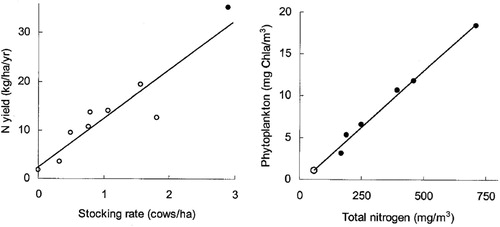
Two regression models provided evidence used to help identify the N load targets for Lake Taupō (Fig. 1); one model related cattle densities in Waikato catchments to catchment N yields (N losses per area of catchment), and the other related water column total N (TN) concentrations with water-column chlorophyll a concentrations in the lake and at downstream sites in the Waikato River (Vant and Huser 2000). Both of these relationships were fitted with linear models, which were robust according to R² coefficients (>0.86). This space-for-stress substitution approach was used to infer a linear S-R relationship shape, but because other lakes sufficiently similar to Lake Taupō do not exist, sites in the Waikato River downstream from Lake Taupō were used to flesh out the relationship. In this way, the S-R framework was implicitly used to derive the N load limits inferred to achieve the stated chlorophyll a target. The N load limit, so determined, has informed land use regulations in the form of the Taupō N cap-and-trade system, which continues to operate in the catchment with the goal of safeguarding the lake.

Case 2: Preventing a regime shift in Waituna lagoon

Waituna Lagoon is an intermittently closed- and open-lake lagoon (referred to henceforth as a lagoon) on the southeast coast of the South Island, New Zealand. Its gravel barrier bar is artificially opened when the lake water level exceeds a trigger level, but the lagoon closes by natural coastal gravel accretion processes. Depending on whether it is open (i.e., in the lagoon state) or closed (i.e., in the lake state) to the sea, the lagoon’s surface area varies between ∼7 and 16 km² and the maximum depth varies between ∼0.7 and 1.7 m (Schallenberg et al. 2010). The lagoon opens about once per year, although this may vary, and over a 25-year period it was closed to the sea 46% of the time (Schallenberg et al. 2010). The lagoon is normally freshwater when full (salinity ∼0.7 psu), but tidal flushing usually raises the salinity of the lagoon to near seawater conditions within a few tidal cycles after the lagoon is open (salinity ∼ 34 psu; Schallenberg et al. 2010). In 2012, the proportion of the catchment of Waituna Lagoon in “high production pasture” was 63% (Rekker and Wilson 2016), mainly comprising dairying, which occupied 44% of the catchment in 2011 (Schallenberg et al. 2017).

The submerged macrophyte community of the lagoon is dominated by 2 seagrasses (Robertson and Funnell 2012), Ruppia megacarpa (R. Mason, 1967) and Ruppia polycarpa (R. Mason, 1967). Seagrass areal cover ranged from 2% to 40% of the lagoon between 2007 and 2016 (Robertson and Funnell 2012; H. Robertson, Department of Conservation, unpubl. data). While the percent macrophyte coverage in Waituna Lagoon varies considerably, the percent coverage including these seagrasses in 2 other east coast South Island lagoons, Lake Ellesmere and Wainono Lagoon, has been severely and persistently reduced to the extent that macrophytes have been virtually absent from the lagoons for decades (Gerbeaux 1993, Schallenberg et al. 2017).

Seagrasses are sensitive to eutrophication (Burkholder et al. 2007), and concern was expressed that recent increases in intensive agriculture in the Waituna catchment could lead to the rapid loss of Ruppia spp. in the lagoon (Waituna Technical Advisory Group 2013). This loss could facilitate regime shifts, first to macroalgal-dominance and eventually to phytoplankton-dominance in the lagoon, similar to the eutrophication trajectory described in Viaroli et al. (2008) and observed in Lake Ellesmere and Wainono Lagoon. To determine nutrient load limits to safeguard Waituna Lagoon from a regime shift, a multiple lines of evidence approach was used to quantify contaminant load thresholds to prevent seagrass loss and eutrophication (Waituna Technical Advisory Group 2013, Schallenberg et al. 2017).

Figure 1. Illustration of the space-for-stress substitution (also known as the space-for-time substitution) approach for determining stressor–response relationships for Lake Taupō. Left panel: catchment nitrogen yields (the load to a waterbody per hectare of catchment area) vs. dairy cattle stocking rates in the Waikato Region (open circle data from Vant 1999; closed circle data from Wilcock et al. 1999). Right panel: phytoplankton biomass (as indicated by chlorophyll a) vs. total nitrogen concentration in Lake Taupō (open circle) and also downstream, in the Waikato River (closed circles). Graphs are reproduced from Vant and Huser (2000) with permission.

One of the lines of evidence involved a literature review of published studies examining drivers of seagrass loss in lagoons and coastal embayments in other parts of the world. The literature review employed the cross-site comparison approach by comparing S-R relationships from different lagoons and embayments to estimate a stressor level threshold to safeguard against seagrass extirpation in Waituna Lagoon (Fig. 2). Burkholder et al. (2007) reviewed seagrass responses to eutrophication from multiple studies, many of which demonstrated S-R relationships derived from a space-for-stress substitution approach (e.g., see figures 7, 11, 12a in Burkholder et al. 2007). Their study revealed logarithmic relationships between seagrass cover or biomass versus N loading, with little evidence of stabilising feedbacks or resistance at low levels of N loading. The nonlinear relationships showed that in many studies, seagrasses were extirpated or reduced to insignificant biomass or cover when certain N loading limits were exceeded.

Figure 2. Cross-site comparison approach showing lagoon area-specific nitrogen (N) loading thresholds below which seagrasses are sustained in lagoons and coastal embayments, as reported from a number of studies (black bars). The lagoon area-specific N loading rates for the New Zealand lagoons Waituna Lagoon (grey bar), Te Waihora/Lake Ellesmere, and Wainono Lagoon (white bars) are also shown. At the time of the study, seagrasses in Waituna Lagoon were under threat, while they had virtually disappeared from the other 2 lagoons.

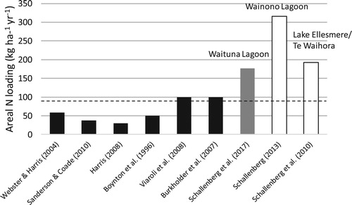
The nonlinear, logarithmic relationship was confirmed by numerous other studies using various approaches to identify S-R relationships and thresholds (Fig. 2), including (1) data from 31 lagoons from New South Wales, Australia, presented in Sanderson and Coade (2010); (2) seagrass data from Harris (2008), who summarised results from mesocosms, in situ experiments, and the deterministic model of Webster and Harris (2004); (3) data on seagrasses and N loading from coastal bays (Boynton et al. 1996); and (4) data in Viaroli et al. (2008), who compiled data from Valiela et al. (1997) and Dahlgren and Kautsky (2004). Thus, the data in these studies confirmed a generalised negative logarithmic S-R relationship relating N loading to seagrass cover/biomass, with N loading thresholds for seagrass collapse that varied somewhat among the studies, but all were ≤100 kg ha⁻¹ yr⁻¹ (Fig. 2).

The second line of evidence used for setting an N load limit to safeguard seagrasses in Waituna Lagoon involved a space-for-stress substitution approach in which relationships between nutrient loads and the trophic states of 57 coastal lagoons and lakes in New South Wales were used to estimate the maximum N load to Waituna Lagoon that could sustain moderate lagoon health, defined as showing some signs of eutrophication but still supporting “healthy seagrass and fish communities” (Scanes 2012). Using this approach, an N loading limit for Waituna Lagoon of 90 kg ha⁻¹ yr⁻¹ was recommended to sustain these values.

The third line of evidence used coupled hydrodynamic and ecological deterministic models to assess the effects of 3 nutrient loading scenarios on the macrophyte biomass in the lagoon (Jones et al. 2018). The model outputs indicated that the calculated nutrient loads (both N and P) to the lake were a threat to the macrophyte biomass in Waituna Lagoon, and the authors concluded that a reduction of 50% of the N load (to 89 kg ha⁻¹ yr⁻¹) and a reduction of 25% of the P load provided an effective level of protection of the seagrass community of the lagoon.

The mean annual N load to Waituna Lagoon was estimated to be 177 kg ha⁻¹ yr⁻¹ (Waituna Technical Advisory Group 2013, Schallenberg et al. 2017), which far exceeded the thresholds to safeguard the seagrasses inferred from these studies (Fig. 2). Furthermore, the N loads estimated for the 2 New Zealand lagoons that had experienced macrophyte die-offs and persistent devegetated states were also well above the thresholds inferred to safeguard the seagrasses in Waituna Lagoon.

Thus, an expert panel judged the 3 independent lines of evidence and recommended an N threshold of 90 kg ha⁻¹ yr⁻¹ to safeguard Waituna Lagoon from a potential regime shift (Waituna Technical Advisory Group 2013, Schallenberg et al. 2017). While the analyses of Scanes (2012) and Jones et al. (2018) also addressed P load limits for Waituna Lagoon, the literature review revealed almost exclusively relationships between N loads and seagrass declines, suggesting consensus that eutrophication of estuarine and coastal systems is more likely to be N limited than P limited (Howarth 1988, Burkholder et al. 2007, Viaroli et al. 2008). While P loads are likely also important in many estuaries (Howarth 1988, Paerl 2009), the available data pool from which to infer an S-R relationship for P loading is currently much smaller.

Case 3: Eutrophication recovery dynamics in seasonally stratified Lake Hayes

Lake Hayes is a eutrophic, monomictic lake with a surface area of 276 ha, a maximum depth of 32 m, and a theoretical water residence time of ∼3.8 years. The lake is located in the Otago Province of the South Island, New Zealand. The lake became eutrophic in the 1960s, and by the 1970s the lake had regular, severe phytoplankton blooms and reduced water clarity, and its hypolimnion showed persistent summer anoxia, with coincident releases of P from the hypolimnetic sediments (Mitchell and Burns 1981, Bayer et al. 2008). Despite its eutrophic condition, the lake is important for its scenic beauty and recreation, although its recreational fishing value has declined in recent years (Schallenberg and Schallenberg 2017).

Bayer et al. (2008) described a lake management strategy implemented in 1995, which, among other protections for the lake, decommissioned septic tanks from dwellings near the lake. In addition, agricultural stocking rates and P fertiliser use in the catchment had declined, which reduced the external nutrient loads to the lake. The reduction of external P inputs seems to have facilitated a slow reduction of the internal P load, as is apparent from the decrease over time of summer hypolimnetic P concentrations (Fig. 3). Nevertheless, phytoplankton blooms and low water clarity in the lake persisted, with phytoplankton blooms again worsening beginning around 2005, as the dinoflagellate Ceratium hirundinella (O.F. Müller; F. Dujardin, 1841) became the dominant bloom-forming phytoplankter in the lake.

Figure 3. Total phosphorus (P) concentration during the seasonal stratified period in the epilimnion (surface; open circles) and in the hypolimnion (25 m; closed circles) in Lake Hayes from 1983 to 2016. Lines are indicative of time trends and were fit to the data using polynomial least squares linear regression. Data are from Jolly (1952, 1959); Burns and Mitchell (1974); Caruso (2001); Otago Regional Council (unpubl. data); CW Burns, University of Otago (unpubl data); and M. Schallenberg (unpubl. data).

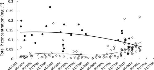
Motile dinoflagellates, such as C. hirundinella, can migrate vertically in the water column to take up P from hypolimnetic waters (James et al. 1992). The existence of a dinoflagellate nutrient “pump” may explain why dinoflagellates often bloom in lakes that have experienced reductions in nutrient loading (Jeppesen et al. 2005) and why they became a nuisance phytoplankter in Lake Hayes as hypolimnetic P concentrations and, by inference the internal P load, declined (Fig. 3). However, in the austral summers of 2009/2010, 2017/2018, and 2018/2019, C. hirundinella did not bloom. As a result, the lake exhibited high levels of water clarity not previously reported in the historical Secchi disk depth record for this lake, which extends back to the late 1940s, well before phytoplankton blooms and anoxia had been reported (Fig. 4). Thus, the putative C. hirundinella-mediated internal nutrient “pump” was apparently inhibited in those recent summers, during which Secchi disk depths were markedly high and C. hirundinella was sparse in the lake.

Figure 4. Available monthly summer (Nov–Apr) water clarity (Secchi disk depth) measurements in Lake Hayes from February 1948 to April 2019. Blooms of Ceratium hirundinella (O. F. Müller; F. Dujardin 1841) were first observed in the lake in 2005; it was the dominant phytoplankter in 2007 and in subsequent bloom years. The solid line shows the time trend fitted by polynomial least squares regression, excluding the measurements from recent clear-water summers (2009/2010, 2016/2017, 2017/2018), fitted by a linear least squares regression (dashed line).

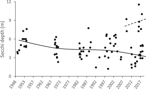
While high nutrient availability had been driving high phytoplankton biomass and low water clarity during the lake’s eutrophication period, Schallenberg and Schallenberg (2017) hypothesised that a decrease in the internal nutrient load by the summer of 2009/2010 was sufficient to manifest a regime shift to an extremely clear water phase that summer. Furthermore, since the summer of 2009/2010, summer water clarity has exhibited large and irregular interannual variability, and Schallenberg and Schallenberg (2017) hypothesised that the lake was in a bifurcation phase, as can occur when a lake repeatedly shifts between alternative stable states (Scheffer 2004).

One explanation for the recent apparent bifurcation in water clarity state is that P availability in the lake has decreased and other factors have begun to control phytoplankton biomass in some years. Thus, using a historical observation approach, a bifurcation dynamic was inferred to explain the complex dynamic exhibited by Lake Hayes as it recovers from high P loads.

While, not commonly reported for seasonally stratifying lakes, nonlinear dynamics, regime shifts, and alternative stable states have previously been reported for 2 such lakes (e.g., Roelke et al. 2007, Carpenter and Lathrop 2008) and inferred for another (Bruel et al. 2018). The analysis of the recent water clarity dynamics in terms of a logistic S-R relationship with hysteresis provides a plausible explanation of the unexpected dynamic of phytoplankton biomass and water clarity, leading to an investigation of the pelagic food web of the lake to determine whether food web biomanipulation could facilitate the recovery of the lake to a stable clear water state (author’s unpubl. data).

Diverse S-R relationship shapes are related to eutrophication

The 3 case studies presented inferred 3 different S-R relationships for 3 different types of lake eutrophication problems (Fig. 5). Each inferred S-R relationship was supported by empirical stressor and response data (either from the case study lakes or from comparable lakes). In addition, information on the presence/absence of feedback mechanisms in the lakes that could affect the shapes of the S-R relationships was also relevant to the selection of appropriate S-R relationships in these case studies.

Figure 5. Conceptual illustration of 3 inferred S-R relationships as applied to 3 lakes with eutrophication problems. Uncertainty about the exact shape of the S-R relationship for Waituna Lagoon (b) is indicated by the 2 lines, showing that the correct relationship could be either logarithmic (continuous line) or logistic (dashed line). See text for explanations.

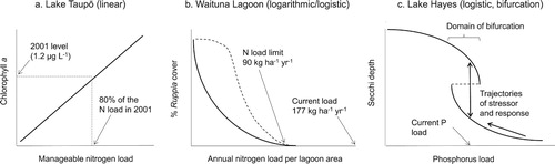
In the case of Lake Taupō, Vant and Huser (2000) presented empirical data that suggested linear relationships between stressors and response, indicating the lack of strong feedback in the pelagic zone of this oligotrophic deep lake. This finding is consistent with Vollenweider (1975), who showed that lakes with long hydraulic residence times (Lake Taupō’s is ∼10.5 yr) were more sensitive to nutrient loading than lakes with shorter residence times.

By contrast, the various studies summarised (Fig. 2) all indicate that that seagrasses in lagoons respond nonlinearly to N loading, showing apparent N load thresholds related to seagrass collapse. Some of the space-for-stress relationships indicated a logarithmic relationship, with little resistance exhibited by the seagrass community to the negative effects of N loading, even at low N loading levels (Valiela et al. 1997, Burkholder et al. 2007). However, conceptual models of seagrass decline in relation to nutrient loading tend to show some seagrass resistance, or even seagrass growth, in the low range of nutrient loading (e.g., Burkholder et al. 2007, Viaroli et al. 2008). While nonlinearity and thresholds are well supported (e.g., Petraitis and Dudgeon 2005, Webster and Harris 2004, Viaroli et al. 2008, Scanes 2012), some uncertainty exists regarding the degree of resistance that seagrasses exhibit in relation to nutrient loading. The uncertainty regarding the degree of resistance is acknowledged by the inclusion of 2 S-R relationships for seagrasses (Fig. 5b), a logarithmic relationship reflecting no resistance and a logistic relationship reflecting some resistance.

S-R relationships derived from single systems may be more informative of ecosystem dynamics than those derived from multi-lake datasets because the degree of ecological resistance and resilience to stressors likely differs among lagoons. However, in the absence of appropriate historical data, S-R relationships derived from multiple systems may still be useful in assessing S-R relationship parameters for a given lagoon, although caution should be exercised in interpreting relationships derived from space-for-stress (i.e., space-for-time) substitutions (Peterson 1984, Capon et al. 2015, Larned and Schallenberg 2018).

In Lake Hayes, a progressive reduction in the internal P load, coincident with the recent development of a marked bifurcation in summer water clarity, suggests the additional influence of at least one other factor in determining summer water clarity. Schallenberg and Schallenberg (2017) suggested that the mediating factor may involve a trophic cascade linking perch recruitment success (i.e., young of the year perch numbers), perch predation on Daphnia, and Daphnia grazing on C. hirundinella. Interannual variability in perch recruitment, and hence in the strength of the trophic cascade, could explain the recent bifurcation among 2 alternative states in Lake Hayes. If these trophic interactions are strong enough to regulate summer water clarity in the lake, then food web biomanipulation to sustain larger Daphnia populations during summer could be a useful restoration activity to facilitate the return of the lake to a stable clear water condition. If the proposed logistic S-R relationship (Fig. 5c) for this lake is correct, both further reductions in P availability and/or alteration to the food web structure would eventually be expected to facilitate a stable recovery of the lake to a clear water state in summer (Jeppesen et al. 1997).

In each of the case studies presented, different approaches were used to infer the appropriate S-R relationships, including space-for-stress substitutions, cross-site comparisons, and historical observations (as described in Larned and Schallenberg 2018). While the deterministic modelling approach for Waituna Lagoon only simulated 4 different N load scenarios (Jones et al. 2018), by testing more N load scenarios a more detailed S-R relationship for that system could also be developed using the deterministic modelling approach.

Toward a lake typology based on S-R relationships

To utilise the S-R framework for accurate lake forecasting, managers should accurately identify a minimum of 4 high-level attributes of systems of interest: (1) the key response variable(s) of the system, (2) the key stressor variable(s) of the system, (3) the current and likely future trajectory of the stressor level(s), and (4) the appropriate form of S-R relationship that governs the dynamics of the system. Guidance on selecting appropriate stressor and response variables is provided in Larned and Schallenberg (2018) and previously discussed works. A trend analysis of historical stressor data may be used to ascertain the trajectory of the stressor level(s). Where direct measures of stressors are unavailable, proxies or indirect measures (e.g., land use, hypolimnetic P concentrations) could be used.

Larned and Schallenberg (2018) described 4 approaches to help correctly infer the most appropriate form of S-R relationship for a given aquatic ecosystem. The approaches require either historical data or stressor and response data from other similar lakes along a stressor gradient. Alternatively, where such data are sparse or lacking, a classification system or typology could facilitate the identification of the appropriate S-R relationship shape for a given lake. To date, relatively few studies have reported actual S-R relationships for lakes. Nevertheless, with the existing data, we propose a preliminary lake typology that relates S-R relationship shapes to eutrophication dynamics in different lake types (Table 1). If such a typology were to be validated, it would imply that certain determinants of the eutrophication process consistently result in certain S-R relationship shapes in certain types of lakes. As such, it could be used by researchers and lake managers to identify key parameters (e.g., sensitivity, thresholds, hysteresis) underpinning eutrophication dynamics in specific lake types, as envisaged by Larned and Schallenberg (2018). Thus, a validated typology could lead the way to more accurate prediction of eutrophication responses to changing stressor levels in lakes.

Table 1. A proposed typology relating lake types to shapes of stressor–response (S-R) relationships in the context of eutrophication.

Lake type	Stressor/response	Form of S-R relationship	Examples	References
Shallow, polymictic	Nutrient availability/water clarity	Logistic with bifurcation and hysteresis^a	Dutch lakes Diverse shallow lakes	Scheffer (2004), Capon et al. (2015)
Medium depth, seasonally stratifying lakes with anoxic hypolimnia	Nutrient availability/water clarity and phytoplankton biomass	Logistic with bifurcation and hysteresis Logistic Logistic with hysteresis	Lake Hayes Lake Kinneret Lake Mendota	Schallenberg and Schallenberg (2017) Roelke et al. (2007), Carpenter and Lathrop (2008)
Deep oligotrophic lakes	Nutrient availability/phytoplankton biomass	Linear	Lake Taupō	Vant and Huser (2000)
Brackish lakes and lagoons	N loading/seagrass cover	Exponential with extinction threshold	Coastal brackish lakes, lagoons and embayments	Schallenberg et al. (2017)

^aLake Taihu, China, may be an exception (see Janssen et al. 2017).

While logistic-type S-R relationships have often been reported for shallow, polymictic lakes, they have rarely been reported for seasonally stratifying lakes (but see Roelke et al. 2007, Carpenter and Lathrop 2008, Bruel et al. 2018). However, seasonally stratifying lakes that develop anoxic hypolimnia may share a eutrophication dynamic with some shallow lakes because the transfer of nutrients from sediments to the water column (benthic–pelagic coupling) is enhanced in both types of lakes (Schallenberg and Burns 2004, Scheffer 2004). In addition, during periods of extended hypolimnetic anoxia, fish and zooplankton may be excluded from hypolimnetic waters, intensifying pelagic trophic interactions in the mixed layer.

Thus, feedback mechanisms conferring nonlinearity and hysteresis in such lakes may include hypolimnetic anoxia and associated internal nutrient loading (e.g., Bush et al. 2017), blooms of vertically motile phytoplankton (e.g., James et al. 1992), and trophic cascades affecting phytoplankton biomass (e.g., Anttila et al. 2013).

By contrast, a linear S-R relationship between N loading and phytoplankton biomass was inferred for Lake Taupō by Vant and Huser (2000), which implies no, or very weak, ecological resistance and stabilising feedbacks with respect to nutrient loads in this lake. Although their data had some limitations, their analysis contributed to the implementation of an N cap-and-trade allocation system to reduce N losses from the catchment to the lake. However, more recent data from Lake Taupō show that while N loads have continued to increase (because of substantial groundwater time lags in the catchment), phytoplankton biomass has not (Vant 2013), possibly because of a shift of phytoplankton from N-limited growth to P-limited growth in recent times. An apparent decoupling of phytoplankton biomass from N concentrations and N loading in the lake highlights that mediating factors and/or multiple stressors may now influence phytoplankton biomass in this lake. Phytoplankton growth and proliferation in lakes is often limited by both N and P (Schindler 2006, Abell et al. 2010, Lewis et al. 2011) and sometimes by micronutrients (e.g., B, Co, Cu, and Mo; Downs et al. 2008), highlighting that attempts to control phytoplankton growth by limiting a single nutrient are not likely to succeed in the long term, especially if the relative availability of different nutrients for phytoplankton growth changes over time (Lewis et al. 2011).

In lagoons, a common eutrophication dynamic involves the sudden loss of seagrasses and other macrophytes, suggesting a strong nonlinear relationship between N loading and macrophyte cover/biomass (Valiela et al. 1997, Burkholder et al. 2007). However, other factors can mediate the eutrophication responses of seagrasses, either via their direct impacts on seagrasses or indirectly via facilitation of macroalgae and phytoplankton biomass accrual. Such factors include variations in salinity, the frequency and durations of barrier bar openings (and the resultant flushing of lagoon water), and sediment loading to lagoons (Haines et al. 2006, Schallenberg et al. 2010). For example, the water residence time (the inverse of the hydraulic flushing rate) of lakes is an important mediator of eutrophication of both seasonally stratified (Vollenweider 1975) and shallow polymictic (Kenny and Waters 2019) lakes. Water residence time seems to have an important mediating role in the areal P loading threshold that differentiates turbid, devegetated shallow lakes from clear, macrophyte-dominated shallow lakes (Kenny and Waters 2019).

Summary and conclusions

The S-R framework for understanding plant productivity has been around since von Liebig’s law of the minimum. Its application to lake management began in the 1970s with the advent of Vollenweider input–output models and has progressed to the compelling alternative stable states model of Scheffer et al. (1993), a logistical S-R relationship with hysteresis that describes the degradation and recovery dynamics of shallow lakes in the context of eutrophication. As some researchers have noted, this model is just one of a variety of different S-R relationships that can be relevant to aquatic ecosystems (Hunsicker et al. 2016, Litzow and Hunsicker 2016, Janssen et al. 2017, Larned and Schallenberg 2018, Ratajczak et al. 2018). The 3 case studies described here demonstrate how different S-R relationships have informed lake management in relation to eutrophication and illustrate how appropriate S-R relationship shapes for given lakes can be inferred from different types of data and information. Different types of lakes seem to be governed by different types of S-R relationships, and S-R relationship types for specific lake types seem to be somewhat consistent. Thus, a lake typology is proposed, which, if validated by further study, could improve the prediction of lake responses to changes in eutrophication drivers.

The S-R relationship framework for lake management described here focuses only on bivariate S-R relationships, but the existence of nonlinear S-R relationships implies that more than one factor can mediate the S-R relationships. For example, lake water residence time, trophic cascades, invasive species, and dual nutrient control of primary production are all known to influence eutrophication. Scheffer (2004) extended bivariate S-R relationship theory into 3 dimensions, and recently Ratajczak et al. (2018) emphasised the importance of multiple stressors and drivers in determining ecosystem responses to change. The extension of S-R relationships to include multiple interacting stressors and responses should improve our ability to predict both simple and complex responses to the multiple changing stressor levels that increasingly affect so many lakes and other types of ecosystems on our changing planet.

Acknowledgements

The Otago Regional Council kindly provided some of the Lake Hayes data. S. Larned, C. Howard-Williams, and an anonymous reviewer kindly provided insightful comments and suggestions on an earlier draft.

Disclosure statement

No potential conflict of interest was reported by the author(s).

Additional information

Funding

This work was supported by the Our Land and Water National Science Challenge, New Zealand Ministry of Business, Innovation and Employment under grant number C10X1507 and by The Health and Resilience of New Zealand’s Lakes programme funded by the New Zealand Ministry of Business, Innovation and Employment under contract number UOWX1503.

References

- Abell JM, Özkundakci D, Hamilton DP. 2010. Nitrogen and phosphorus limitation of phytoplankton growth in New Zealand lakes: implications for eutrophication control. Ecosystems. 13:966–977. doi: 10.1007/s10021-010-9367-9
- Anttila S, Ketola M, Kuoppamäki K, Kairesalo T. 2013. Identification of a biomanipulation-driven regime shift in Lake Vesijärvi: implications for lake management. Freshwater Biol. 58:1494–1502. doi: 10.1111/fwb.12150
- Bayer T, Schallenberg M, Martin CE. 2008. Investigation of nutrient limitation status and nutrient pathways in lake Hayes, Otago, New Zealand: a case study for integrated lake assessment. New Zeal J Mar Fresh. 42:285–295. doi: 10.1080/00288330809509956
- Boynton WR, Murray L, Hagy JD, Stokes C, Kemp WM. 1996. A comparative analysis of eutrophication patterns in a temperate coastal lagoon. Estuaries. 19:408–421. doi: 10.2307/1352459
- Bruel R, Marchetto A, Bernard A, Lami A, Sabatier P, Frossard V, Perga M-E. 2018. Seeking alternative stable states in a deep lake. Freshwater Biol. 63:553–568. doi: 10.1111/fwb.13093
- Burkholder JM, Tomasko DA, Touchette BW. 2007. Seagrasses and eutrophication. J Exp Mar Biol Ecol. 350:46–72. doi: 10.1016/j.jembe.2007.06.024
- Burns CW, Mitchell SF. 1974. Seasonal succession and vertical distribution of phytoplankton in Lake Hayes and Lake Johnson, South Island, New Zealand. New Zeal J Mar Fresh. 8:167–209. doi: 10.1080/00288330.1974.9515496
- Bush T, Diao M, Allen RJ, Sinnige R, Muyzer G, Huisman J. 2017. Oxic-anoxic regime shifts mediated by feedbacks between biogeochemical processes and microbial community dynamics. Nat Comm. 8:1–9. doi: 10.1038/s41467-016-0009-6
- Capon SJ, Lynch AJJ, Bond N, Chessman BC, Davis J, Davidson N, Finlayson M, Gell PA, Hohnberg D, Humphrey C, Kingsford RT. 2015. Regime shifts, thresholds and multiple stable states in freshwater ecosystems; a critical appraisal of the evidence. Sci Total Environ. 534:122–130. doi: 10.1016/j.scitotenv.2015.02.045
- Carpenter SR, Lathrop RC. 2008. Probabilistic estimate of a threshold for eutrophication. Ecosystems. 11:601–613. doi: 10.1007/s10021-008-9145-0
- Caruso BS. 2001. Risk-based targeting of diffuse contaminant sources at variable spatial scales in a New Zealand high country catchment. J Env Manag. 63:249–268. doi: 10.1006/jema.2001.0476
- Dahlgren S, Kautsky L. 2004. Can different vegetative states in shallow coastal bays of the Baltic Sea be linked to internal nutrient levels and external nutrient loads? Hydrobiologia. 514:249–258. doi: 10.1023/B:hydr.0000018223.26997.b0
- Dillon PJ, Rigler FH. 1974. The phosphorus–chlorophyll relationship in lakes. Limnol Oceanogr. 19:767–773. doi: 10.4319/lo.1974.19.5.0767
- Downs TM, Schallenberg M, Burns CW. 2008. Responses of lake phytoplankton to micronutrient enrichment: a study in two New Zealand lakes and an analysis of published data. Aquat Sci. 70:347–360. doi: 10.1007/s00027-008-8065-6
- Duhon M, McDonald H, Kerr S. 2015. Nitrogen trading in Lake Taupo: an analysis and evaluation of an innovative water management policy. Motu working paper 15-07. Wellington (NZ): Motu Economic and Public Policy Research; 56 p.
- Gaedke U, Straile D. 1998. Daphnids: keystone species for the pelagic food web structure and energy flow – a body size-related analysis linking seasonal changes at the population and ecosystem levels. Adv Limnol. 53:587–610.
- Gerbeaux P. 1993. Potential for re-establishment of aquatic plants in Lake Ellesmere (New Zealand). J Aquat Plant Manag. 31:122–128.
- Haines PE, Tomlinson RB, Thom BG. 2006. Morphometric assessment of intermittently open/closed coastal lagoons in New South Wales, Australia. Est Coast Shelf Sci. 67:321–332. doi: 10.1016/j.ecss.2005.12.001
- Harris GP. 2008. Supplementary information to support final report recommendation No. 2. ACWS Technical Note No. 2. Prepared for the Adelaide Coastal Waters Study Steering Committee. Hobart Tasmania: ESES Systems Pty Ltd.
- Howarth RW. 1988. Nutrient limitation of net primary production in marine ecosystems. Ann Rev Ecol. 19:89–110. doi: 10.1146/annurev.es.19.110188.000513
- Hunsicker ME, Kappel CV, Selkoe KA, Halpern BS, Scarborough C, Mease L, Amrhein A. 2016. Characterizing driver–response relationships in marine pelagic ecosystems for improved ocean management. Ecol Appl. 26:651–663. doi: 10.1890/14-2200
- James WF, Taylor WD, Barko JW. 1992. Production and vertical migration of Ceratium hirundinella in relation to phosphorus availability in Eau Galle Reservoir, Wisconsin. Can J Fish Aquat Sci. 49:694–700. doi: 10.1139/f92-078
- Janssen ABG, de Jager VCL, Janse JH, Kong X, Liu S, Ye Q, Mooij WM. 2017. Spatial identification of critical nutrient loads of large shallow lakes: implications for Lake Taihu (China). Water Res. 119:276–287. doi: 10.1016/j.watres.2017.04.045
- Jeppesen E, Lauridsen T, Mitchell SF, Burns CW. 1997. Do planktivorous fish structure the zooplankton communities in New Zealand lakes? New Zeal J Mar Fresh. 31:163–173. doi: 10.1080/00288330.1997.9516755
- Jeppesen E, Søndergaard M, Jensen JP, Havens KE, Anneville O, Carvalho L, Coveney MF, Deneke R, Dokulil MT, Foy B, et al. 2005. Lake responses to reduced nutrient loading – an analysis of contemporary long-term data from 35 case studies. Freshwater Biol. 50:1747–1771. doi: 10.1111/j.1365-2427.2005.01415.x
- Jolly VH. 1952. A preliminary study of the limnology of Lake Hayes. Aust J Mar Fresh Res. 3:74–91. doi: 10.1071/MF9520074
- Jolly VH. 1959. A limnological study of some New Zealand lakes [dissertation]. Dunedin (New Zealand): University of Otago.
- Jones HFE, Özkundakci D, McBride CG, Pilditch CA, Allan MG, Hamilton DP. 2018. Modelling interactive effects of multiple disturbances on a coastal lake ecosystem: implications for management. J Env Manage. 207:444–455. doi: 10.1016/j.jenvman.2017.11.063
- Jørgensen SE. 1976. A eutrophication model for a lake. Ecol Model. 2:147–165. doi: 10.1016/0304-3800(76)90030-2
- Kenny WF, Waters MN. 2019. Exploring the influence of hydrology on the threshold phosphorus-loading rate in shallow lakes. Watershed Ecol Env. 1:10–14. doi: 10.1016/j.wsee.2019.03.001
- Larned ST, Schallenberg M. 2018. Stressor–response relationships and the prospective management of aquatic ecosystems. New Zeal J Mar Fresh. 51:78–95.
- Lehman JT, Botkin DB, Likens GE. 1975. The assumptions and rationales of a computer model of phytoplankton population dynamics. Limnol Oceanogr. 20:343–364. doi: 10.4319/lo.1975.20.3.0343
- Lehmann MK, Hamilton DP. 2018. Modelling water quality to support lake restoration. Chapter 3 In: Hamilton DP, Collier, KJ, Quinn JM, Howard-Williams CH, editors. Lake restoration handbook. Dordrecht (Netherlands): Springer Nature; p. 67–106.
- Lewis WM, Wurtsbaugh WA, Paerl HW. 2011. Rationale for control of anthropogenic nitrogen and phosphorus to reduce eutrophication of inland waters. Env Sci Technol. 45:10300–10305. doi: 10.1021/es202401p
- Litzow MA, Hunsicker ME. 2016. Early warning signals, nonlinearity, and signs of hysteresis in real ecosystems. Ecosphere. 7:e01614. doi: 10.1002/ecs2.1614
- Mitchell SF, Burns CW. 1981. Phytoplankton photosynthesis and its relation to standing crop and nutrients in two warm-monomictic South Island lakes New Zeal J Mar Fresh. 15:51–67. doi: 10.1080/00288330.1981.9515897
- [OECD] Organisation for Economic Development and Co-operation. 2015. The Lake Taupo nitrogen market in New Zealand: a review for policy makers. Lessons in environmental Policy Reform. OECD Environment Policy Paper, No. 4. Paris (France).
- Pace ML, Carpenter SR, Cole JJ. 2015. With and without warning: managing ecosystems in a changing world. Front Ecol Environ. 13:460–467. doi: 10.1890/150003
- Paerl HW. 2009. Controlling eutrophication along the freshwater-marine continuum: dual nutrient (N and P) reductions are essential. Estuar Coast. 32:593–601. doi: 10.1007/s12237-009-9158-8
- Peterson CH. 1984. Does a rigorous criterion for environmental identity preclude the existence of multiple stable points? Am Nat. 124:127–133. doi: 10.1086/284256
- Petraitis PS, Dudgeon SR. 2005. Detection of alternative stable states in marine communities. J Exp Mar Biol Ecol. 326:14–26. doi: 10.1016/j.jembe.2005.05.013
- Ratajczak Z, Carpenter SR, Ives AR, Kucharik CJ, Ramiadantsoa T, Stegner MA, Williams JW, Zhang J, Turner MG. 2018. Abrupt change in ecological systems: inference and diagnosis. Trends Ecol Evol. 33:513–526. doi: 10.1016/j.tree.2018.04.013
- Redfield AC. 1958. The biological control of chemical factors in the environment. Am Sci. 46:205–221.
- Rekker J, Wilson S. 2016. Waituna catchment water quality review. Report 1051-3-R1. Lincoln (NZ): Lincoln Agritech Ltd.; [accessed Oct. 14, 2019]. https://www.waituna.org.nz/repository/libraries/id:1ytnyjmap17q9s20wg7s/hierarchy/Waituna%20resources/Catchment%20management/2016%2005%20Rekker%20Waituna%20Catchment%20Water%20Quality%20Review.pdf
- Rigler FH, Peters RH. 1995. Science and limnology. Excellence in Ecology Vol 6. Oldendorf/Luhe (Germany): International Ecology Institute. 239 p.
- Robertson HA, Funnell EP. 2012. Aquatic plant dynamics of Waituna Lagoon, New Zealand: trade-offs in managing opening events of a Ramsar site. Wetl Ecol Manag. 20:433–445. doi: 10.1007/s11273-012-9267-1
- Roelke DL, Zohary T, Hambright KD, Montoya JV. 2007. Alternative states in the phytoplankton of lake Kinneret, Israel (Sea of Galilee). Freshwater Biol. 52:399–411. doi: 10.1111/j.1365-2427.2006.01703.x
- Sanderson B, Coade G. 2010. Scaling the potential for eutrophication and ecosystem state in lagoons. Environ Model Softw. 25:724–736. doi: 10.1016/j.envsoft.2009.12.006
- Scanes P. 2012. Nutrient loads to protect environmental values in Waituna Lagoon, Southland, New Zealand. Report prepared for Environment Southland. Invercargill: Environment Southland; [accessed Sept 28, 2019]. https://www.waituna.org.nz/repository/libraries/id:1ytnyjmap17q9s20wg7s/hierarchy/Waituna%20resources/Lagoon%20management/2012%2005%20Scanes%20Nutrient%20Loads%20to%20Protect%20Environmental%20Values%20in%20Waituna%20Lagoon%20NZ.pdf
- Schallenberg M, Burns CW. 2004. Effects of sediment resuspension on phytoplankton production: teasing apart the influences of light, nutrients, and algal entrainment. Freshwater Biol. 49:143–159. doi: 10.1046/j.1365-2426.2003.01172.x
- Schallenberg M, Hamilton DP, Hicks AS, Robertson HA, Scarsbrook M, Robertson B, Wilson K, Whaanga D, Jones HFE, Hamill K. 2017. Multiple lines of evidence determine robust, 2019 nutrient load limits required to safeguard a threatened lake/lagoon system. New Zeal J Mar Fresh. 51:78–95. doi: 10.1080/00288330.2016.1267651
- Schallenberg M, Larned ST, Hayward S, Arbuckle C. 2010. Contrasting effects of managed opening regimes on water quality in two intermittently closed and open coastal lakes. Est Coast Shelf Sci. 86:587–597. doi: 10.1016/j.ecss.2009.11.001
- Schallenberg M, Schallenberg LA. 2017. A restoration and monitoring strategy for Lake Hayes. Report prepared for the Friends of Lake Hayes Society; [accessed September 28]. https://yoursay.orc.govt.nz/38718/documents/111850
- Scheffer M. 2004. The ecology of shallow lakes. Dordrecht (Netherlands): Kluwer Academic Publishers. 356 p.
- Scheffer M, Hosper SH, Meijer ML, Moss B, Jeppesen E. 1993. Alternative equilibria in shallow lakes. Trends Ecol Evol. 8:275–279. doi: 10.1016/0169-5347(93)90254-M
- Schindler DW. 1971. Carbon, nitrogen and phosphorus and the eutrophication of freshwater lakes. J Phycol. 7:321–329. doi: 10.1111/j.1529-8817.1971.tb01527.x
- Schindler DW. 1987. Detecting ecosystem responses to anthropogenic stress. Can J Fish Aquat Sci. 44(Suppl. 1):s6–s25. doi: 10.1139/f87-276
- Schindler DW. 2006. Recent advances in the understanding and management of eutrophication. Limnol Oceanogr. 51:356–363. doi: 10.4319/lo.2006.51.1_part_2.0356
- Stow CA, Cha YK. 2013. Are chlorophyll a–total phosphorus correlations useful for inference and prediction. Environ Sci Technol. 47:3768–3773. doi: 10.1021/es304997p
- Timperley MH. 1983. Phosphorus in spring waters of the Taupo Volcanic zone, North Island, New Zealand. Chem Geol. 38:287–306. doi: 10.1016/0009-2541(83)90060-8
- Valiela I, McClelland J, Hauxwell J, Behr PJ, Hersh D, Foreman K. 1997. Macroalgal blooms in shallow estuaries: controls and ecophysiological and ecosystem consequences. Limnol Oceanogr. 42:1105–1118. doi: 10.4319/lo.1997.42.5_part_2.1105
- Vallentyne JR. 1974. The algal bowl. Ottawa (ON): Department of the Environment. 154 p.
- Vant B. 1999. Sources of nitrogen and phosphorus in several major rivers in the Waikato region. Environment Waikato Technical Report 1999/10. Hamilton (NZ): Environment Waikato.
- Vant B. 2013. Recent changes in water quality of Lake Taupo and its inflowing streams. New Zeal J For Sci. 58:27–30.
- Vant B, Huser B. 2000. Effects of intensifying catchment land-use on the water quality of Lake Taupo. Proc New Zeal Soc An Prod. 60:261–264.
- Viaroli P, Bartoli M, Giordani G, Naldi M, Orfanidis S, Zaldivar JM. 2008. Community shifts, alternative stable states, biogeochemical controls and feedbacks in eutrophic coastal lagoons: a brief overview. Aquat Conserv. 18(S1):S105–S117. doi: 10.1002/aqc.956
- Vollenweider RA. 1968. Scientific fundamentals of the eutrophication of lakes and flowing waters, with particular reference to nitrogen and phosphorus as factors in eutrophication. Technical Report DAS/CS/68.27. Paris (France): OECD.
- Vollenweider RA. 1975. Input-output models with special reference to the phosphorus loading concept in limnology. Schweiz Z Hydrobiol. 37:53–84.
- Vollenweider RA. 1976. Advances in defining critical loading levels for phosphorus in lake eutrophication. Mem Ist Ital Idrobiol. 33:53–83.
- Waituna Technical Advisory Group. 2013. Ecological guidelines for Waituna Lagoon. Invercargill (NZ): Environment Southland; [accessed Sept. 28, 2019]. https://www.researchgate.net/publication/311736375_Ecological_Guidelines_for_Waituna_Lagoon
- Webster IT, Harris GP. 2004. Anthropogenic impacts on the ecosystems of coastal lagoons: modelling fundamental biogeochemical processes and management implications. Mar Freshwater Res. 55:67–78. doi: 10.1071/MF03068
- White E, Downes M, Gibbs M, Kemp L, Mackenzie L, Payne G. 1980. Aspects of the physics, chemistry, and phytoplankton biology of Lake Taupo. New Zeal J Mar Fresh. 14:139–148. doi: 10.1080/00288330.1980.9515855
- Wilcock RJ, Nagels JW, Rodda HJE, O’Connor MB, Thorold BS, Barnett JW. 1999. Water quality of a lowland stream in a New Zealand dairy farming catchment. New Zeal J Mar Fresh. 33:683–696. doi: 10.1080/00288330.1999.9516911