Projected changes of regional lake hydrologic characteristics in response to 21st century climate change

ABSTRACT

Inland lakes are socially and ecologically important components of many regional landscapes. Exploring lake responses to plausible future climate scenarios can provide important information needed to inform stakeholders of likely effects of hydrologic changes on these waterbodies in coming decades. To assess potential climate effects on lake hydrology, we combined a previously published spatially explicit, processed-based hydrologic modeling framework implemented over the lake-rich landscape of the Northern Highlands Lake District within the United States with an ensemble of climate change scenarios for the 2050s (2041–2070) and 2080s (2071–2100). Model results quantify the effects of climate change on water budgets and lake stage elevations for 3692 lakes and highlight the importance of landscape and hydrologic setting for the response of specific lake types to climate change. All future climate projections resulted in loss of ice cover and snowpack as well as increased evaporation, but variability in climate projections (warmer conditions, wet winters combined with wet or dry summers) interacted with lake characteristics and landscape position to produce variable lake hydrologic changes. Water levels for drainage lakes (lakes with substantial surface water inflows and outflows) showed nearly no change, whereas minimum water levels for seepage lakes (minimal surface water fluxes) decreased by an average of up to 2.64 m by the end of the 21st century. Our physically based modeling approach is parsimonious and computationally efficient and can be applied to other lake-rich regions to investigate interregional variability in lake hydrologic response to future climate scenarios.

KEYWORDS:

• climate change
• groundwater
• hydrologic change
• lake response
• surface water

Introduction

Interactions between climate and local hydrologic characteristics influence lake and reservoir processes that are ecologically and societally important. These interactions influence globally relevant biogeochemical processes (Cole et al. 2007, Raymond et al. 2013, Schmadel et al. 2019) and affect lake levels and water budgets with implications for ecologically important littoral habitats and riparian zones (Perales et al. 2020). Despite a general awareness of the importance of lakes and reservoirs, currently a large void exists regarding the understanding of the hydrologic effects of a changing climate on inland lakes, especially over large spatial and temporal scales.

Most studies exploring the effects of future changes in climate on lake hydrological and biogeochemical properties fit into 2 broad approaches. The first focuses on large-scale analyses of trends from historical observations (e.g., Magnuson et al. 1997, O’Reilly et al. 2015) and coarse estimates of physical processes (e.g., Cardille et al. 2007, 2009). The second approach focuses on small-scale analyses projecting the response of individual lakes. Hunt et al. (2013) performed detailed modeling of the Trout Lake watershed in northern Wisconsin, United States, simulating lake stages, lake water budgets, and groundwater levels in the surrounding aquifer, and Hamilton et al. (2018) applied a detailed hydrodynamic lake-ice model to a single seepage lake in the same Trout Lake watershed to project lake thermodynamics, ice cover, and lake stage under climate change. The detailed and physically based approach of Hunt et al. (2013) successfully captures heterogeneous lake responses, but it is computationally demanding to perform over large spatial areas. Furthermore, it requires extensive model parameterization and calibration supported by detailed field observations, meaning that the cost of simulating the response of a large number of lakes at regional or larger scales is prohibitive. Studies that use both these approaches have applied either wet or dry perturbation scenarios using historically observed wet and dry values (Cardille et al. 2009) or future climate forcing datasets (Hunt et al. 2013) that have since been updated with estimations of future climate that more accurately capture the estimated climate trajectory and range of variability of improved climate modeling (Hayhoe et al. 2017).

The field is poised to take the next step in regional-scale analyses of hydrologic responses to future climate. However, remaining challenges for lake hydrology models include both capturing heterogeneous lake responses from first principles and performing analyses across large spatial scales under historical conditions and projected future climate scenarios. Other researchers have called for increased observation and experimental networks that focus on improving our collective knowledge of inland lakes and reservoirs (Williamson et al. 2008, 2009, Moss 2012). In addition to direct benefits of increased observations and controlled experiments in understanding lake behavior, such efforts could also help provide data to validate and refine process-based modeling approaches. Although some of the methods that use statistical models based on historical relationships to evaluate future effects are promising, research efforts should also continue to design and implement spatially explicit, process-based models to investigate the response of individual lakes over large spatial scales (e.g., Hanson et al. 2018, Zwart et al. 2018).

Climate model advancements over the past decade provide opportunities to investigate more extensively how future climate conditions may affect regional scale inland water resources. Current climate models have improved model representation of climate, and a greater number of models are now available that can help span the variability and uncertainty that come with predictive modeling (Taylor et al. 2012). Parsimonious and computationally efficient hydrologic models are also needed to explore the potential effects of future climate on changes in water resources using the most up-to-date climate scenarios to help water resources managers prepare for future conditions. We created a modeling framework that combines a relatively simple and computationally efficient modeling approach developed and validated in our region of interest (Hanson et al. 2018). Our model is driven by statistically downscaled climate change forcing datasets developed for the Midwest and Great Lakes region (Byun and Hamlet 2018). Using this integrated modeling framework, we investigated the detailed hydrologic effects of climate change on 3692 lakes in the northern Midwest, United States. Our modeling framework accounts for a number of lake-specific characteristics, enabling investigation of how different lake types and lakes in aggregate will respond to a changing climate. With these model experiments we aimed to characterize the hydrologic heterogeneity in the response of specific lake types and quantify and explore the effects of climate change on water budgets, residence time, and lake stage across an interconnected regional landscape. Although we focus on a specific region in this case study, the approach and methods are broadly applicable to other inland lake systems.

Materials and methods

Study domain and modeling overview

As a regional case study, we simulated the Northern Highlands Lake District (NHLD) located in a forested and largely undeveloped portion of northern Wisconsin and Michigan, United States (Fig. 1). The NHLD covers ∼6000 km². We simulated 3692 lakes and reservoirs ranging in size from 0.06 to 220 000 ha, and of these, 506 had inflowing streams and 3186 had no inflowing streams. Our study used the modeling framework developed by Hanson et al. (2018), which had previously been validated for a representative portion of the region. The hydrology model (Hanson et al. 2018) used a computationally efficient integrated surface water/groundwater (SW/GW) modeling framework coupled to a lake water budget (LWB) model incorporating daily time-step inputs and exports from individual lakes within the simulated domain (discussed later). In the previous study, simulated lake responses of long-term hydrological and biogeochemical compared well with observations over historical climate for a subset of lakes within the NHLD (Hanson et al. 2018, Zwart et al. 2018). With this region as our continued testbed, we investigated the hydrological response of the lakes under scenarios of projected future climate change.

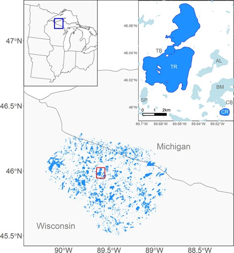
Figure 1. The 3692 lakes and reservoirs simulated for this current study are within the Northern Highlands Lake District (NHLD), located in northern Wisconsin and Michigan, United States. Two of the lakes highlighted in this study, Trout Lake (TR) and Crystal Lake (CR), are within 3.5 km of each other (top right inset map). The remaining North Temperate Lakes Long Term Ecological Research lakes (Allequash Lake, AL; Big Muskellunge Lake, BM; Sparkling Lake, SP) and bogs (Crystal Bog, CB; Trout Bog, TB) are also displayed.

Historical meteorological driving data

Previous model simulations using historical meteorological forcing data (Hanson et al. 2018) formed the baseline for the climate change experiments in this study, and the output of Hanson et al. (2018) is compared with the output of the present study. The historical gridded meteorological forcing dataset over the Midwest and Great Lakes region included daily total precipitation, maximum and minimum temperature data from station records, and simulated wind speed data from large-scale global reanalysis simulations. See Hanson et al. (2018) and Byun and Hamlet (2018) for additional details.

Climate change scenarios

To simulate future conditions, the lake hydrology model was forced with statistically downscaled daily temperature (T) and precipitation (P) data using the Hybrid Delta (HD) downscaling approach (Hamlet et al. 2013, Tohver et al. 2014) applied over the Midwest and Great Lakes region of the United States and Canada (Byun and Hamlet 2018). The HD downscaling process in Byun and Hamlet (2018) can be thought of as superimposing projections of future climate extracted from 30-year windows in the future onto 99 years of observed climate variability (1915–2013). Thus, for the HD downscaling approach, the 2050s and 2080s represent global climate model (GCM) simulated changes in climate for 30-year time periods, centered on the decade noted (2041–2070 and 2071–2100, respectively), superimposed on historical climate variability (1915–2013).

The final spatial resolution after downscaling was 1/16th of a degree and the temporal resolution of climate forcings was daily. The HD downscaled future projections are explicitly indexed to the historical record, which allows interpretation of the results of future scenarios using the knowledge of past weather and climate events (Byun and Hamlet 2018). We used 6 GCM scenarios from the Coupled Model Intercomparison Project Phase 5 (CMIP5; Taylor et al. 2012) that performed well across the Midwest and Great Lakes region and reproduced the range of changes in T and P for the full ensemble of 31 GCMs (Byun and Hamlet 2018). We used these 6 representative climate scenarios for the 2050s (2041–2070) and 2080s (2071–2100) time periods for the representative concentration pathway (RCP) RCP8.5 emission scenario, resulting in 12 individual scenarios for our future analysis. RCP8.5 is the highest or “business as usual” (Taylor et al. 2012) greenhouse gas (GHG) concentration scenario used in the CMIP5. These scenarios are an update and improvement from earlier climate change scenarios (CMIP3; Taylor et al. 2012) used in related studies (Hunt et al. 2013). We use the highest GHG concentration scenario because it compares well with current emissions trajectories (Hayhoe et al. 2017, Schwalm et al. 2020).

The projections, which are based on a delta-method concept, are explicitly indexed to the historical period 1915–2013 and have the same sample size as the historical datasets (99 years) in all cases. To compare the time series of historical values and future projections on the same plot, we adopted the convention of plotting results according to the historical dates to which the future projections are indexed.

Coupled surface water and groundwater hydrology model

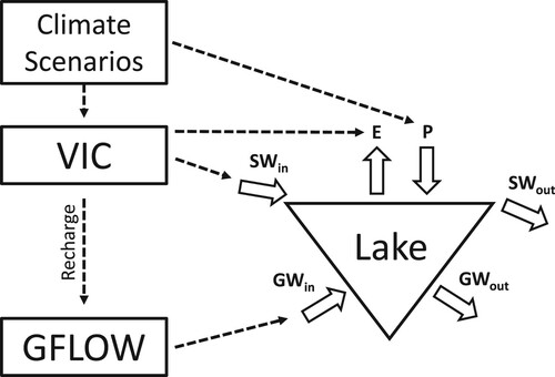
The hydrology model uses an integrated SW/GW modeling framework that combines the Variable Infiltration Capacity (VIC) land surface hydrology model (Liang et al. 1994), the GFLOW analytic element method GW model (Haitjema 1995), and an LWB model (Hanson et al. 2018). Our modeling framework simulated the daily changes of water storage within each individual lake due to water flux inputs and exports that are informed by the SW and GW models (Fig. 2). VIC solved the land surface energy and water balance for each 1/16th degree grid cell across the modeling domain at daily time-steps, which includes simulating surface runoff, base flow, open water evaporation, and GW recharge. VIC was one-way coupled to our GW model, GFLOW, which solved the 2-dimensional steady-state GW equation given the variable inputs of lake surface elevation and estimated GW recharge from VIC. Because GFLOW is an analytic element method, we represented lakes as discretized polygons that served as the individual analytic elements and boundary conditions for GFLOW. The GW model was broken into subdomains based on the Watershed Boundary Dataset 12-digit hydrologic units (HUC12s; https://water.usgs.gov/GIS/huc.html) in which VIC flux data from VIC grid cells that are partially within the HUC12 subdomain boundary are averaged to provide a single input file of daily values. During the model simulation, GFLOW estimated GW discharge into and out of each lake by summing the GW discharges at each segment of the lakes’ shorelines. We estimated daily lake surface elevation by calculating the water balance for each lake using the hydrologic inputs and outputs estimated from our coupled SW/GW model and a lake area to volume relationship estimated from a subset of lakes in our modeling domain.

Figure 2. Conceptual figure of the modeling framework used for this study and described in more detail in Hanson et al. (2018). The 12 different climate change scenarios (6 GCMs for both the 2050s and the 2080s climate) drove simulations of the land surface hydrology model (VIC), which simulated recharge to the groundwater aquifer and stream flow into each lake (SW_in). The groundwater model (GFLOW) was one-way coupled to VIC and used simulated recharge and lake stage to estimate groundwater inflow (GW_in) and outflow (GW_out) to and from each lake. Lake surface precipitation (P) was simulated from the climate scenarios and lake evaporation (E) was simulated by VIC. Surface outflow (SW_out) was simulated as a linear reservoir and dependent on lake stage. Additionally, lake ice cover was simulated by VIC and lake evaporation was turned off when lake ice was present. At each time step, the lake water budget model (LWB) calculated changes in lake volume and surface elevation using the hydrologic inputs and outputs.

Because VIC simulates water information based on climate, the only aspect that changed within our hydrologic modeling framework from the historical to the future simulations was the meteorological forcing data input to VIC, created by Byun and Hamlet (2018). Historical simulations in Hanson et al. (2018) ran through water year (WY) 2015, but the Byun and Hamlet (2018) HD datasets used for this study only extended through WY 2013 (1915–2013), resulting in a total period simulated for this study from WY 1980 to 2013 (1 Oct 1979 to 30 Sep 2013). All lake basin characteristics and morphometry parameterization were the same as detailed in Hanson et al. (2018), using modifications for a subset of lakes and bogs (n = 7) described in the discussion section of that work. As part of our analysis, effective lake surface precipitation minus potential evaporation from open water (P-E) was calculated by setting potential evaporation from open water to zero when simulated lake ice was present.

Primary drivers of changing lake evaporation and evapotranspiration over land

VIC uses the well-known Penman equation and Penman-Monteith equation to simulate lake (open water) evaporation and evapotranspiration over land, respectively. Evaporation in the simulations is directly affected by warming (via increases in the saturated vapor pressure), decreasing separation between daily minimum air temperature (T_min) and daily maximum air temperature (T_max) used in the VIC model to estimate attenuation of solar radiation by clouds (using the MTCLIM model incorporated in VIC; Thornton and Running 1999), and increasing T_min, which is used to estimate the dewpoint temperature in VIC (also using MTCLIM). Ice cover is also a significant driver of lake evaporation, and changes in this variable are explicitly simulated by the LWB model (discussed earlier). Changes in vegetation and wind speed also potentially affect evapotranspiration, but changes in these variables were not included in our future projections (climate and land cover uncertainties discussed later).

Thus, in the future projections, lake evaporation and evapotransporation over land tend to increase strongly due to warming and loss of ice cover alone, but these effects are tempered by decreased solar radiation (increased cloudiness following more rapid changes in T_min than in T_max that reduces the spread between T_min and T_max) and increased dew point temperature and humidity (following increasing T_min). These changes are believed to reflect plausible future scenarios for the 3 primary variables affecting evaporation included in the study.

Analysis of hydrological responses at regional and local scales

We hypothesized that projected changes in climate result in a wide range of hydrologic changes, including decreases in lake ice cover and snowpack accumulation, changes in the timing of runoff in streams and GW recharge, increases in the volume of precipitation and runoff during the winter and spring months, and increases in lake surface evaporation during the summer months. To address our goal to investigate the variable responses of lake hydrologic characteristics and budget changes at both regional and local scales, we present results relating to the entire NHLD region (3692 total lakes simulated across ∼6000 km²) as well as 2 well-studied lakes, Trout and Crystal, which are part of the North Temperate Lakes Long Term Ecological Research (NTL-LTER; Magnuson et al. 2006; https://lter.limnology.wisc.edu/). The NTL-LTER includes 5 lakes and 2 bogs located within the NHLD (Fig. 1). Trout and Crystal lakes are in close proximity (lake boundaries separated by <3.5 km; Fig. 1) but have strikingly different hydrological characteristics (Hunt et al. 2013, 2014, 2018). Trout Lake is a large drainage lake, having substantial SW inflows and outflows, while Crystal Lake is a small seepage lake (having minimal surface water inflows or outflows) located in the uplands of the Trout Lake watershed. Despite the high contrast in their hydrologic characteristics, our model performed well for these lakes when compared to historical observations (Hanson et al. 2018, Zwart et al. 2018). By looking at the specific hydrologic responses to a changing climate of these 2 representative lakes, we can more easily investigate the individual components of coupled GW and SW interactions to illustrate the response of different lake types to climate change across the region as a whole.

For the analysis of individual lakes as well as regional (or global) lake populations, we focused on 2 key metrics. First, we estimated hydrologic residence time (HRT = V/Q), where HRT is hydrologic residence time (t), V is volume (L³) where L is the length scale as estimated by Hanson et al. (2018), and Q is total volumetric inflow of all water sources (L³/t). HRT is important because it characterizes the time available for processing nutrients and carbon arriving from the surrounding landscape through water pathways for a given lake. Because HRT is proportional to volume and inversely proportional to inflows, changes in either of these within a lake’s water budget are important for understanding this quantity. Second, fraction of hydrologic export as evaporation (FHEE) is a useful metric for understanding local lake hydrologic characteristics with total exports from a lake considered as the summation of open water evaporation and outflowing GW and surface water. For lakes more hydrologically isolated from the landscape (i.e., seepage lakes), FHEE values are generally higher. Conversely, for lakes that are less hydrologically isolated from the landscape (i.e., drainage lakes), FHEE values are generally lower. See Hanson et al. (2018) and Zwart et al. (2018) for more in-depth discussion relating to both HRT and FHEE, and Zwart et al. (2019a) for how changes in FHEE can affect lake productivity and carbon processing.

Examining changes in the water balance associated with changes in direct P to the lake surface, evaporation from the lake surface (E), and net streamflow inputs from surface water (net SW) and groundwater (net GW) helps clarify the underlying drivers for the stage responses discussed earlier. To normalize units, various fluxes are presented as long-term mean volumes normalized by each lake’s historical average lake area (i.e., cm of depth over the average historical lake area). The change in future values relative to the historical baseline values (future–historic) is illustrated by changes in P and E from our model and were equal for all of the NTL-LTER lakes, but changes in the surface area of each lake in response to climate change varies, which affects direct P to the lake surface and E from the lake surface to some extent (Hanson et al. 2018). We note that net SW and net GW can be substantially different for different lakes.

Results and discussion

Summary of projected changes in climate over the NHLD

The NHLD is projected to experience steadily increasing annual average temperatures and total precipitation over the 21st century (Fig. 3). In the RCP8.5 scenarios, temperature increased across all months by an average of 3.79 °C for the 2050s and 6.26 °C for the 2080s (Fig. 4a). Long-term mean monthly precipitation totals for the entire NHLD (baseline for WYs 1980–2013) are projected to increase during the cool season (Nov–Mar) by 15% and 25% for the 2050s and the 2080s, respectively. Essentially all climate models show increases in precipitation for these months. Mean warm season (Jul–Sep) precipitation, by comparison, remained about the same in the 2050s and decreased by nearly 7% in the 2080s (Fig. 4b), with large variability among the different GCMs. Conditions in late summer (Aug–Sep), however, showed more systematic drying across scenarios. These results indicate large systematic increases in precipitation in the cool season, but that summer conditions may vary from decade to decade, encompassing both wet and dry conditions relative to a historical baseline at different times.

Figure 3. Inter-model variability of annual average changes in temperature (°C) and precipitation (%) across the NHLD over the simulated 34-year period for the 6 GCM projections chosen, representative of the 2080s period for the 6 GCM scenarios considered. The symbols align with figure 5 in Byun and Hamlet (2018).

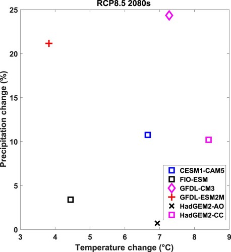
Figure 4. Monthly composite mean values of the 6 GCMs and VIC simulation output used across the NHLD for (a) air temperature, (b) precipitation, (c) first-day-of-month (only non-composite mean value) snow water equivalent, (d) watershed evapotranspiration, (e) effective lake surface precipitation minus potential evaporation over open water (P-E; E = 0 when lake ice is present), (f) watershed precipitation minus evapotranspiration (P-ET), (g) streamflow (base flow plus surface runoff), and (h) net groundwater recharge. Mean changes under future climate forcings are shown in the solid lines for the 2050s and the 2080s with the minimum and maximum bounds shown by respective shaded coloring.

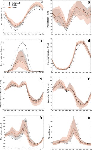
Despite increases in annual P totals for all simulations, only 5 of the 12 individual climate scenarios showed an increase in precipitation minus evapotranspiration (P-ET) across the NHLD region compared to historical values (GFDL-CM3, GFDL-ESM2M, and HadGEM2-CC in the 2050s; GFDL-CM3 and GFDL-ESM2M in the 2080s). Increases in temperature result in projected increases in ET for the region that exceed the projected increases in precipitation. Projected annual average T and P changes for the NHLD align well with watershed-scale projections in southern Wisconsin (Hunt et al. 2016) and also with the broader Great Lakes and Midwest region from other studies (Winkler et al. 2012, Pryor et al. 2014).

Surface hydrology response to changing T and P over the NHLD

Hydrologic responses in the simulations were strongly coupled to changes in precipitation from snow to rain in the cool season and loss of snow cover in the spring. Winter and spring peak snow storage (peak first-of-month snow water equivalent in cool season) was strongly affected by warming, with peak values reduced by 49% and 63% for 2050s and 2080s, respectively, and the peak shifted about 1 month earlier at the end of the century from March to February (Fig. 4c). Both terrestrial (watershed) evapotranspiration (ET over land; Fig. 4d) and potential evaporation from open water surfaces (E; not shown) followed essentially the same trends as temperature during summer months with maximum increases of 11% by the 2080s. These increases are comparable to projected global changes in lake evaporation from other studies (e.g., Wang et al. 2018).

Long-term-mean monthly effective lake surface precipitation minus potential evaporation from open water (P-E) increased during the cool season (Nov–Mar) by nearly 18% and 30% during the 2050s and 2080s, respectively, and decreased during warm season months (Jul–Sep) by nearly 21% and 54% during the 2050s and 2080s, respectively (Fig. 4e). Similarly, mean monthly watershed precipitation minus evapotranspiration (i.e., P-ET, or watershed runoff; Fig. 4f) increased during the cool season (Nov–Mar) by more than 11% and 18% during the 2050s and 2080s, respectively, and decreased during warm season months (Jul–Sep) by nearly 26% and 46% during the 2050s and 2080s, respectively.

Average monthly net GW recharge to the subsurface increased by a factor of >2.5 from November to March for the 2080s, and springtime peaks in recharge were reduced by 32% and 44% for the 2050s and 2080s, respectively (Fig. 4h). These changes in recharge timing primarily reflect the changes in the amount of snow accumulation and timing of melt (Fig. 4c). For the 2080s, the average dates of peak GW recharge shifted about 1 month earlier from April to March (Fig. 4g). Likewise, total streamflow (base flow and surface runoff; Fig. 4h) followed similar shifts as net recharge, but with the mean peak for both the 2050s and 2080s shifting from May to April and reduced by 22% and 32%, respectively. These changes in the timing and magnitude of spring snowmelt also imply reductions in spring flooding (Byun et al. 2019).

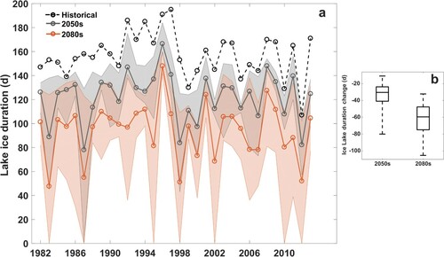
Systematic reductions in ice duration due to warming were seen across all simulations (Fig. 5) and are well aligned with Northern Hemisphere projections for reductions in lake ice (Sharma et al. 2019). Values of lake ice duration for the mean of the 6 GCM ensemble members were reduced by 35 and 63 days for the 2050s and 2080s, respectively. For the relatively warm and dry HadGEM-A0 GCM projections, 7 years had complete loss of ice cover for the 2080s scenarios during the 34-year simulated time period.

Figure 5. (a) Lake ice duration from WYs 1982–2013. Black dashed line shows historical values. Mean changes under future climate forcing are shown in the solid lines, with the minimum and maximum bounds shown by respective shading. (Note that the climate change results are indexed to historical years in the HD downscaling approach). (b) Changes in lake ice duration under future climate scenarios (future mean – historical) with median, 25th percentile, 75th percentile, minimum and maximum values shown with the box and whiskers plots.

Changes in lake levels for different lake types

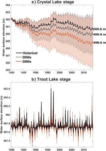
Previous work examining historical trends has demonstrated that drainage lakes and seepage lakes in the NHLD have different hydrologic responses to decadal climate variability (e.g., Hunt et al. 2013, Watras et al. 2014, Hanson et al. 2018). We expected that these fundamental differences would express themselves as heterogeneous responses to a changing future climate as well. A comparison between the results for Crystal Lake, a small seepage lake, and Trout Lake, a larger drainage lake, is instructive (Fig. 6). Crystal Lake shows much greater sensitivity to different GCM scenarios than Trout Lake. The average minimum stage values across the 6 GCM simulations for Crystal Lake are reduced by 0.80 and 2.04 m for the 2050s and 2080s, respectively, compared with only 0.02 and 0.08 m for Trout Lake when compared to each lakes’ historically simulated minimum stage. The HadGEM2-AO GCM scenario (rank 3 for warming and rank 6 for P increase from Fig. 3) showed the greatest loss in stage for Crystal Lake with reductions of 3.44 and 5.31 m for the 2050s and 2080s, respectively, compared with 0.14 and 0.24 m for Trout Lake. Similarly, the GFDL-CM3 GCM scenario (rank 2 for warming and rank 1 for P from Fig. 3) showed the maximum increases in Crystal Lake stage with increased values of about 0.90 m for both the 2050s and 2080s compared with increases of <0.11 m for Trout Lake. These differing sensitivities relate to the strong regulating effect of streams into and out of drainage lakes such as Trout Lake that are not present for seepage lakes such as Crystal Lake. In essence, Trout Lake remains full because future streamflow and GW inputs to the lake are sufficient to compensate for decreases in P-E. By contrast, the absence of streamflow inputs and continual GW loss downgradient means Crystal Lake responds directly and strongly to changes in P-E.

Figure 6. Simulated daily lake surface elevation for historical, 2050s, and 2080s with the mean (bold line) and the minimum and maximum values from the 6 GCM scenarios, shown by the respective shaded coloring over the 34-year simulation period for (a) Crystal Lake and (b) Trout Lake.

Implications of lake-specific hydrologic responses

For Crystal Lake, annual direct P rates increased on average from 94.28 cm/yr to 100.56 and 100.12 cm/yr for the 2050s and 2080s, respectively. Although the average annual precipitation increased on average across the NHLD from the 2050s to the 2080s, volumetric precipitation inputs were actually reduced in Crystal Lake because of the substantial reduction in available lake area as lake stage decreased (Fig. 6a). Compounding this reduction, E rates also increased on average for Crystal Lake, from a historical rate of 85.32 cm/yr to 94.96 and 99.10 cm/yr for the 2 respective time periods. GW inputs for Crystal Lake changed from a baseline value of −13.19 cm/yr (i.e., a net loss) to −11.19 and −9.24 cm/yr for the 2050s and 2080s, respectively (Fig. 7a). For seepage lakes like Crystal Lake (for which SW_in and SW_out are zero), this implies a small negative water balance in the future scenarios, resulting in a reduction in lake stage and surface area as discussed earlier.

Figure 7. Changes in the lake mass balance components associated with direct precipitation (P), evaporation (E), net surface water (SW), and net groundwater (GW) for the 6 GCM scenarios for the 2050s and the 2080s. The mean change value for each period are represented with crosses for (a) Crystal Lake and (b) Trout Lake. Mean volumes were normalized by lake’s historical average lake area. The zero-change line is shown as the dashed black line. For reference, the average historical mass balance component values over the entire simulation time-period are provided for Crystal Lake (P = 94.37 cm/yr; E = 85.32 cm/yr; net SW = 0.00 cm/yr; net GW = −13.19 cm/yr); and Trout Lake (P = 94.35 cm/yr; E = 85.26 cm/yr; net SW = −16.00 cm/yr; net GW = 7.03 cm/yr).

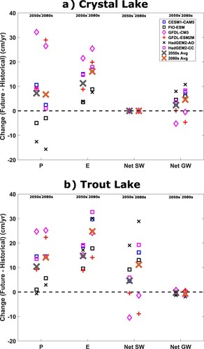
Trout Lake saw differing shifts in P and E when compared to Crystal Lake because on average its lake stage was relatively unaffected in the future (Fig. 6b). Trout Lake also showed relatively small changes in GW rates (positive historical values decreased by 0.24 and 0.56 cm/yr for the 2050s and 2080s, respectively). Trout Lake’s net SW rates increased on average from a historical baseline of −15.99 cm/yr (i.e., a net loss) to −12.03 and −6.41 cm/yr. Trout Lake’s decreases in P-E are essentially matched by reductions in outflow from SW, resulting in only small changes in storage and stage.

The varying changes in net hydrologic fluxes between the 2 lake types (seepage or drainage) also result in changes in individual lake hydrologic characteristics of interest, such as HRT, FHEE, and similar metrics for precipitation and snowmelt, SW flows, and GW flows (Supplemental Table S1). Crystal Lake’s simulated HRT, for example, was reduced across all scenarios, with an average reduction of about 1 year for the 2050s and about 2 years for the 2080s because of systematic decreases in volume (5% and 17% for the 2050s and 2080s, respectively) and increases in inflows (12% and 7% for the 2050s and 2080s, respectively). Trout Lake simulations showed minimal changes in volume (<1%) but a mix of decreases and increases in HRT for different GCMs and time periods, showing small increases in the ensemble average for both the 2050s and 2080s.

Regional-scale summary of hydrologic changes in the NHLD

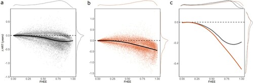
The previous sections detailing the responses to climate change of 2 lakes that historically had different hydrologic characteristics serve as a bridge to help us understand the response of the entire NHLD lake population. Overall, the NHLD future simulations show widespread reductions in HRT for both the 2050s and the 2080s for the average across the 6 GCMs (Supplemental Table S2). These results generally align with the simpler approaches implemented by Cardille et al. (2009), in which wetter simulations decreased the lake average HRTs due to increased inflows. However, in contrast to the increased HRT simulated for dry scenarios by Cardille et al. (2009), our model estimated significant decreases in HRT for dry scenarios. We attribute our simulated decreases in HRT under dry conditions to a substantial reduction in simulated volumes of lakes with higher FHEE values, leading to the overall reduction in HRT across all simulations (Fig. 8). Lakes at different ends of the FHEE spectrum responded differently, with low-FHEE lakes seeing both increases and decreases in HRT while high-FHEE lakes’ HRT was primarily reduced. On average, many lakes in the region show increases in E and FHEE, increases in precipitation, decreases in both inflow and exports of surface water flow, and relatively little change in GW inflow and exports. However, as seen in the different responses of Crystal Lake and Trout Lake to the same changes in future climate, the response of individual lakes in the NHLD is variable. The simulated changes are also sensitive in some cases to the uncertainty in projected future climate, especially precipitation in summer.

Figure 8. Changes in mean lake hydrologic residence time (HRT) relative to the historical mean HRT as a function of fraction of hydrologic export as evaporation (FHEE), displaying mean lake stage change for all 3692 lakes for each of the 6 GCMs for the (a) 2050s climate (gray) and (b) 2080s climate (orange) with respect to their projected FHEE value. The zero-change line is shown as the dashed black line. The solid trend lines show the LOESS best fit line for each time-period. (c) The best fit lines from (a) and (b) at a narrower y-axis range. The marginal plots on each panel represent the density of lakes for changes in HRT (right marginal densities) and period-specific FHEE (top marginal densities). Panel (c) includes the historical FHEE density in the marginal plot shown as a black line.

Surface elevation responses at regional scales

We further explored the overall response of the NHLD lake population to climate change by projecting changes in mean and minimum lake stage relative to historical FHEE values. Across the NHLD, both the changes in the mean stage (Fig. 9) and the minimum stage (Fig. 10) showed considerable variability as a function of FHEE (i.e., lake types) as well as GCM scenarios for individual lakes (Fig. 9b, 10b). Average changes in the minimum lake stage elevation were more pronounced compared to the changes seen in the mean values, and decreases in lake stage all became more pronounced with time (compare 2050s to the 2080s in Table 1). For the most sensitive seepage lakes (generally highest FHEE), reductions in the average of mean lake stage were 0.66 m for the 2050s and 1.41 m for the 2080s (Fig. 9); similarly, the largest reductions in average of minimum lake stage were 1.29 m for the 2050s and 2.64 m for the 2080s (Fig. 10). By comparison, Crystal Lake had a total lake stage range (maximum–minimum) of 1.81 m over its historical observed period from April 1981 to August 2013 in response to decadal climate variability (Fig. 6). These results highlight changes in lake stage as an important effect pathway in the NHLD and highlight an increase in the number of lakes with seepage lake characteristics under climate change.

Figure 9. Changes in mean lake stage relative to the historical mean lake stage, displaying the (a) ensemble mean for 6 GCMs within 100 equally spaced bins of historical FHEE for the 2050s in gray and the 2080s in orange, and (b) mean lake stage change for all 3692 lakes for each of the 6 GCMs under 2050s climate (gray) and 2080s climate (orange) with respect to their historical FHEE value. Symbols relating to individual GCMs are shown in the legend of the inset (b) panel. Locations of the bins containing Trout Lake and Crystal Lake are labeled.

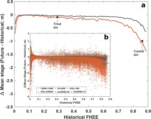
Figure 10. Changes in minimum lake stage relative to the historical minimum lake stage, displaying (a) the ensemble mean for 6 GCMs within 100 equally spaced bins of historical FHEE for the 2050s in gray and the 2080s in orange, and (b) minimum lake stage change for all 3692 lakes for each of the 6 GCMs under 2050s climate (gray) and 2080s climate (orange) with respect to their historical FHEE value. Symbols relating to individual GCMs are shown in the legend of the inset (b) panel. Locations of the bins containing Trout Lake and Crystal Lake are labeled.

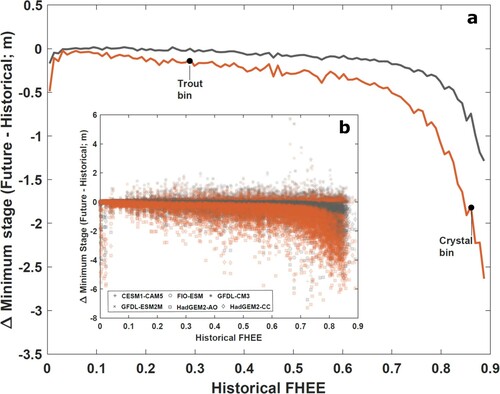
Table 1. Mean and minimum lake stage changes for the average of the 6 GCMs for the 2050s and 2080s scenarios.

Change	Fraction of hydrologic export as evaporation (FHEE)	2050s	2080s
Change of mean stage (m)	FHEE < 0.50	−0.03	−0.09
	FHEE ≥ 0.50	−0.10	−0.29
Change of minimum stage (m)	FHEE < 0.50	−0.03	−0.14
	FHEE ≥ 0.50	−0.19	−0.53

Note: Changes in lake stage calculated as (future – historical).

The results also indicate that uncertainties in changing lake stage are likely to be substantial for seepage lakes in the NHLD. The range of stage projections at the end of the transient simulations for Crystal Lake is on the order of 6.5 m (Fig. 6a), a range ∼3.6 times the normal range associated with decadal variability for Crystal Lake. Similar results are shown for another NTL-LTER study lake, Big Muskellunge Lake (Supplemental Fig. S1).

Implications of the variability and uncertainty of climate projections

Two main points can be taken away from our results showing changes to regional water balance, lake-specific responses, and regional lake population responses:

1. There was a consistent increase in temperature but variable changes in net precipitation (P-E) for plausible future climate projections.

2. For any given climate scenario, the response of the regional lake population was heterogeneous in magnitude, but individual lakes across the entire region generally responded in the same direction as one another (e.g., seepage lakes filled for wet scenarios or drained for dry scenarios).

Across the 2 time periods (2050s and 2080s) and the 6 climate scenarios considered for each (total n = 12), all scenarios showed increases in P over winter and spring months (Dec–May; n = 12), but only half showed increases in P over summer and fall months (Jun–Nov; n = 6). These relationships align with the analysis of Byun and Hamlet (2018) for the Great Lakes and Midwest region as a whole and highlight some key conclusions: (a) there is greater certainty in the cool-season precipitation under future climate, with all GCM projections over the NHLD showing increases in precipitation for RCP8.5; however, (b) uncertainty in warm-season is considerably larger and indicates possible extended periods of wetter or dryer conditions at different times in the future combined with overall wetter conditions in the cool season; and (c) late summer/early fall (Aug–Sep) conditions are more consistently drier in the projections than the summer as a whole. For warm-season projections over the NHLD for the 2050s, 4 of 6 GCMs showed increased P compared to 2 of 6 GCMs in the 2080s, providing some evidence that warm season precipitation could systematically decline toward the end of the 21st century.

Although the hydrologic response of individual lakes varied across the NHLD, all lakes tended to respond in similar directions for a given GCM projection (i.e., a wet GCM projection filled lakes, a dry GCM drained lakes), which can be explained by the underlying processes driving the changes for different lakes. Drainage lakes are substantially affected by surface inflow changes and, accordingly, have similar changes in surface outflows but little change in lake stage. Seepage lakes, however, largely depend on the balance between P and E (P-E). If the balance favors one variable in a future climate scenario more than the other, the seepage LWB and stage elevation will follow consistently across this class of lakes, resulting in substantial changes in lake volume and stage. Because the NHLD is dominated by lakes having seepage-like qualities (FHEE > 0.5), and that number only increases under future climates on average (Fig. 8), the NHLD is expected to experience substantial hydrologic changes under average future climate change, one way (wetter, gaining volume) or the other (drier, losing volume). Increasing terrestrial ET tends to reduce SW inputs and GW recharge. Increasing open water E and reduced ice cover tend to systematically shift P-E toward drier conditions and loss in lake stage (Fig. 4). As noted earlier, these different responses may occur at different times in the future, and future climate may tend toward a higher probability of drier warm season conditions by the 2080s.

Modeling uncertainty and limitations

Our modeling framework was designed to be as physically based as possible, and validation against historical observations in Hanson et al (2018) helped support our results under projected future climate scenarios. However, the underlying modeling framework described by Hanson et al. (2018) has uncertainties and limitations that warrant consideration when interpreting the results, especially when driven by conditions beyond the validation dataset. Although a complete uncertainty analysis is not included here, we briefly review some of the major uncertainties in the modeling framework and discuss their implications in the interpretation of the results presented. We also discuss several limitations of the current modeling framework and thoughts relating to future work that could address limitations.

Hydrologic model uncertainty

Hanson et al. (2018) examined the effect of uncertainty in lake watershed characteristics and lake morphometry on lake hydrologic fluxes and stage. Specifically, for the 7 well-studied NTL-LTER lakes and bogs for which there are confident estimates in lake watershed characteristics and lake morphometry, Hanson et al. (2018) identified some seepage lakes whose simulated watershed characteristics resulted in inflowing SW, despite field knowledge that no inflowing SW was expected to be present. Overestimating SW inflow based on geospatial analysis of watershed area would likely cause simulated lake stage to have reduced variability and underpredict HRT compared to observations, and errors in lake morphometry would cause errors in estimated HRT and, to a lesser extent, lake stage. For example, for 3 NTL-LTER lakes and bogs, Hanson et al. (2018) turned off surface inflows and adjusted volumes to align with published field observations, which resulted in better alignment between simulated HRT and previously published HRT values.

Errors in geospatial data likely have less effect on the simulation of stage for drainage lakes (e.g., Trout Lake) because errors in inflowing hydrologic fluxes mostly affect outflowing hydrologic fluxes and only minimally affect lake stage but would still affect quantities such as estimated lake HRT. When simulated with future climate scenarios, we expect errors in watershed characteristics to have the most effect on simulated changes in seepage lake stage and HRT. However, we do not have enough data to indicate a consistent bias in estimating watershed characteristics (e.g., overestimating SW inflow for seepage lakes, or over/under estimating SW inflow for drainage lakes). Thus, we assumed these kinds of errors are randomly distributed for both historical and future analysis, and we are relatively confident in the simulated regional response for lake stage and HRT under future climate scenarios, even though we may not be as confident in the results for any one lake in particular. Exceptions include the NTL-LTER lakes for which there are long-term data. Lake morphometry estimates are uncertain because available morphometry data are lacking and morphometry is difficult to estimate with precision from available data such as lake area (Oliver et al. 2016). Resulting errors in the simulation of lake volume can substantially influence HRT and FHEE. As mentioned in Hanson et al. (2018), the errors in estimated lake volumes were expected to be randomly distributed across the entire NHLD lake population and across all landscape positions (i.e., both seepage and drainage lakes). Because lake morphometry was kept the same for historical and future climate simulations and errors in lake morphometry were expected to be randomly distributed across lakes, we are relatively confident in the overall trends in lake HRT as a result of climate change as simulated by our model.

The uncertainty of GW discharge estimates to and from lakes is largely coupled with, and driven by, the uncertainty of the SW components of the model. For example, errors in SW components will cause the model to either over or under predict lake stage depending on the direction of the inflowing SW estimate error. This error in the lake stage estimate will affect the estimate of lake GW exchange with the GW aquifer. For example, if SW inflows were over predicted, the resulting increased stage would tend to reduce inflowing GW and increase outflowing GW. It is uncertain whether the effects to HRT due to these potential errors as the increased GW outflow would work to counteract an increase in volume; however, GW discharge responses are muted by hydraulic conductivity of the surrounding aquifer and respond more slowly than surface processes. Again, we do not have enough data to know if there are systematic errors in SW fluxes that would affect GW fluxes; thus, we assume regional trends in GW fluxes are randomly distributed and projected regional trends in response to climate scenarios are not significantly biased by these effects.

Uncertainties due to initial lake stage

The initial conditions of the lakes in our future model runs were all set to the same historical lake surface elevation that Hanson et al. (2018) used as initial conditions. Developing improved methods for initializing lake stages under future conditions, however, would likely improve our understanding of long-term lake conditions of large lake populations, especially related to the long-term response of seepage lakes under climate change.

Climate uncertainty due to uncertain GHG concentration trajectory

In part based on limited global GHG mitigation efforts to date, we have focused here on RCP8.5 as a plausible high-end GHG concentration scenario. However, uncertain human choices could ultimately play a critical role in determining actual GHG concentrations at the end of the century and the effects on Midwest climate. Byun and Hamlet (2018), for example, showed that regional warming for RCP4.5 (a “middle of the road” GHG scenario) is approximately half the projected warming for RCP8.5 in the Midwest. Seasonal precipitation changes are broadly similar in character for RCP4.5 and RCP8.5 (i.e., wetter winters, uncertain summers) but are lagged in time for RCP4.5. Precipitation changes for RCP4.5 for the 2080s, for example, are broadly comparable to RCP8.5 for the 2050s. Thus, there is considerable uncertainty about the timing of changes in temperature and precipitation but a strong consensus from the GCMs about, for example, direction of change and seasonal patterns of changes in each variable. The range of uncertainty between GCMs is less for RCP4.5 for a given time frame, as well. Thus, lake simulations for RCP4.5 for the 2080s would be about the same as those for RCP8.5 for the 2050s.

Modeling uncertainties due to future land cover

Our modeling framework maintains current landscape vegetation coverage across all time periods. How future agriculture and forest vegetation will respond to the large increases in temperature simulated by GCMs as well as the shifts in precipitation and available water quantity during the warm season is currently poorly understood but has important implications for studies of this kind. Land use within the NHLD is dependent on many largely unknown variables, including future decisions made by the public, land managers, and policy makers with regard to agriculture, forest management, and stewardship of the lakes themselves. Future scenarios of vegetation change could be incorporated in the VIC model to explore these issues using our existing modeling framework. With these uncertainties in mind, the research presented here is useful in helping to inform outreach efforts to help stakeholders, natural resource managers, and policy makers to envision future effects to these important natural resources.

Opportunities to extend the modeling framework to encompass larger spatial scales

Our modeling approach was developed to be computationally efficient and can be applied in any setting where necessary model setup and forcing data are available. Our methodology would be appropriate to use and apply at continental scales, or even globally. To further test the portability of this current modeling framework, the application of our modeling approach under both historical and future climates to additional lake-rich regions is important, as is investigating other subcontinental-scale regions such as mountainous landscapes, high latitude areas, and semiarid environments. An example of more expansive analysis that would be beneficial is the extension of this modeling framework to the entirety of the lake-rich temperate regions of North America, where the landscape features are similar to those of the NHLD presented here. Our current modeling framework can easily be parallelized to be efficiently applied to these larger regions.

Summary and conclusions

Our research combined a previously published integrated hydrologic modeling framework implemented over the NHLD (Hanson et al. 2018) with an ensemble of 21st century climate change scenarios for the 2050s and 2080s (Byun and Hamlet 2018). Our modeling framework is parsimonious, computationally efficient, and process-based, allowing application at much larger scales (continental and global), provided model parameters (e.g., lake area, watershed area, land cover) and meteorological forcing data are available. Our study results highlight the heterogeneity in the hydrologic response of specific lake types and quantify the effects of climate change on water availability (water budgets and lake stage elevations) for nearly 4000 lakes in the NHLD.

• Upland seepage lakes (high FHEE) showed the greatest sensitivity to widespread reductions in P-E in the climate change scenarios, and many of these lakes are projected to shrink in volume, stage, and surface area in the future. Most of the GCM scenarios showed systematic reductions in P-E over the NHLD, so this finding has relatively high certainty.

• Drainage lakes (low FHEE) are relatively insensitive to changes in P-E and show little change in stage in the simulations because streamflow inputs and outputs effectively compensate for changes in P-E.

With variable future climate projections (warmer conditions, wet winters combined with wet or dry summers), the regional lake population responded in the simulations with a wide range of hydrologic changes; however, the magnitude and type of individual lake responses was largely dependent on the lake characteristics and position within the landscape. Thus, quantitative metrics such as FHEE (based on observations or simulations) can be used to characterize the likely effects of climate change on the water availability and water quality (Zwart et al. 2019a) of different lakes by identifying those historically with predominantly drainage or seepage lake characteristics.

Acknowledgements

The authors thank Dr. Kyuhyun Byun for providing access to downscaled GCM data over the Midwest region and discussing the future climate scenarios and methodologies. We thank the 2 anonymous reviewers and Dr. Noah Schmadel for comments that improved this manuscript. Thanks also to Dr. Chun Mei Chiu for access to the Midwest US implementation of the VIC model and historical meteorological driving data sets. VIC simulations were run with the support of the University of Notre Dame’s Center for Research Computing. Any use of trade, firm, or product names is for descriptive purposes only and does not imply endorsement by the US Government.

Data availability

In addition to the Supplemental Materials, data associated with this article can be found at several previously reported locations. Readers are directed to supporting information related to the hydrologic lake modeling source code in Hanson et al. (2018) and for historical and future projected meteorological forcing data to Byun et al. (2019; please contact the lead author of the cited report for access to datasets). Lastly, lake hydrologic modeling output analyzed in this publication is described by Zwart et al. (2019b).

Disclosure statement

No potential conflict of interest was reported by the author(s).

Additional information

Funding

This work was supported by the National Science Foundation [grant number: EAR-1351623, EAR-PF-1725386, and DEB-1547866].

References

- Byun K, Chiu CM, Hamlet AF. 2019. Effects of 21st century climate change on seasonal flow regimes and hydrologic extremes over the Midwest and Great Lakes region of the US. Sci Total Environ. 650:1261–1277.
- Byun K, Hamlet AF. 2018. Projected changes in future climate over the Midwest and Great Lakes region using downscaled CMIP5 ensembles. Int J Climatol. 38:e531–e553.
- Cardille JA, Carpenter SR, Coe MT, Foley JA, Hanson PC, Turner MG, Vano JA. 2007. Carbon and water cycling in lake-rich landscapes: landscape connections, lake hydrology, and biogeochemistry. J Geophys Res. 112(G2).
- Cardille JA, Carpenter SR, Foley JA, Hanson PC, Turner MG, Vano JA. 2009. Climate change and lakes: estimating sensitivities of water and carbon budgets. J Geophys Res. 114:G03011.
- Cole JJ, Prairie YT, Caraco NF, McDowell WH, Tranvik LJ, Striegl RG, Duarte M, Kortelainen P, Downing JA, Middelburg JJ, Melack J. 2007. Plumbing the global carbon cycle: integrating inland waters into the terrestrial carbon budget. Ecosystems. 10(1):172–185.
- Haitjema HM. 1995. Analytic element modeling of groundwater flow. Cambridge (MA): Academic Press.
- Hamilton DP, Magee MR, Wu CH, Kratz, TK. 2018. Ice cover and thermal regime in a dimictic seepage lake under climate change. Inland Waters, 8(3):381–398.
- Hamlet AF, Elsner MM, Mauger GS, Lee SY, Tohver I, Norheim RA. 2013. An overview of the Columbia basin climate change scenarios project: approach, methods, and summary of key results. Atmos Ocean. 51(4):392–415.
- Hanson PC, Buffam I, Rusak JA, Stanley EH, Watras C. 2014. Quantifying lake allochthonous organic carbon budgets using a simple equilibrium model. Limnol Oceanogr. 59(1):167–181.
- Hanson ZJ, Zwart JA, Vanderwall J, Solomon CT, Jones SE, Hamlet AF, Bolster D. 2018. Integrated, regional-scale hydrologic modeling of inland lakes. J Am Water Res Assoc. 54(6):1302–1324.
- Hayhoe K, Edmonds J, Kopp RE, LeGrande AN, Sanderson BM, Wehner MF, Wuebbles DJ. 2017. Climate models, scenarios, and projections. In: Wuebbles DJ, DW Fahey, KA Hibbard, DJ Dokken, BC Stewart, TK Maycock, editors. Climate science special report: Fourth national climate assessment, Volume I. Washington, DC: US Global Change Research Program; p. 133–160.
- Hunt RJ, Walker JF, Selbig WR, Westenbroek SM, Regan RS. 2013. Simulation of climate-change effects on streamflow, lake water budgets, and stream temperature using GSFLOW and SNTEMP, Trout Lake watershed, Wisconsin. US Geol Surv Sci Invest Rep. 2013–5159. doi:https://doi.org/10.3133/sir20135159
- Hunt RJ, Westenbroek SM, Walker JF, Selbig WR, Regan RS, Leaf AT, Saad DA. 2016. Simulation of climate change effects on streamflow, groundwater, and stream temperature using GSFLOW and SNTEMP in the Black Earth Creek watershed, Wisconsin. US Geol Surv Sci Invest Rep. doi:https://doi.org/10.3133/sir20165091
- Liang X, Lettenmaier DP, Wood EF, Burges SJ. 1994. A simple hydrologically based model of land surface water and energy fluxes for general circulation models. J Geophys Res. 99(D7):14415–14428.
- Magnuson JJ, Kratz TK, Benson BJ, editors. 2006. Long-term dynamics of lakes in the landscape – long-term ecological research on north temperate lakes. New York (NY): Oxford University Press.
- Magnuson JJ, Webster KE, Assel RA, Bowser CJ, Dillon PJ, Eaton JG, Schindler DW. 1997. Potential effects of climate changes on aquatic systems: Laurentian Great Lakes and Precambrian shield region. Hydrol Processes. 11(8):825–871.
- Moss B. 2012. Cogs in the endless machine: lakes, climate change and nutrient cycles: a review. Sci Total Environ. 434:130–142.
- Oliver SK, Soranno PA, Fergus CE, Wagner T, Winslow LA, Scott CE, Stanley EH. 2016. Prediction of lake depth across a 17-state region in the United States. Inland Waters. 6(3):314–324.
- O’Reilly CM, Sharma S, Gray DK, Hampton SE, Read JS, Rowley RJ, Weyhenmeyer GA. 2015. Rapid and highly variable warming of lake surface waters around the globe. Geophys Res Lett. 42(24):10–773.
- Perales KM, Hein CL, Lottig NR, Vander Zanden MJ. 2020. Lake water level response to drought in a lake-rich region explained by lake and landscape characteristics. Can J Fish Aquat Sci. 77(11):1836–1845.
- Pryor S, Scavia D, Downer C, Gaden M, Iverson L, Nordstrom R, Patz J, Roberson G. 2014. Midwest climate change impacts. US Third Nat Climate Assessment; p. 418–440.
- Raymond PA, Hartmann J, Lauerwald R, Sobek S, McDonald C, Hoover M, Kortelainen P. 2013. Global carbon dioxide emissions from inland waters. Nature. 503(7476):355–359.
- Schmadel NM, Harvey JW, Schwarz GE, Alexander RB, Gomez-Velez JD, Scott D, Ator SW. 2019. Small ponds in headwater catchments are a dominant influence on regional nutrient and sediment budgets. Geophys Res Lett. 46(16):9669–9677.
- Schwalm CR, Glendon S, Duffy PB. 2020. RCP8. 5 tracks cumulative CO2 emissions. P Natl Acad Sci USA. 117(33):19656–19657.
- Sharma S, Blagrave K, Magnuson JJ, O’Reilly CM, Oliver S, Batt RD, Magee MR, Straile D, Weyhenmeyer GA, Winslow L, Woolway RI. 2019. Widespread loss of lake ice around the Northern Hemisphere in a warming world. Nat Clim Change. 9(3):227–231.
- Taylor KE, Stouffer RJ, Meehl GA. 2012. An overview of CMIP5 and the experiment design. Bull Am Meteorol Soc. 93(4):485–498.
- Thornton PE, Running SW. 1999. An improved algorithm for estimating incident daily solar radiation from measurements of temperature, humidity, and precipitation. Agric For Meteorol. 93(4):211–228.
- Tohver IM, Hamlet AF, Lee SY. 2014. Impacts of 21st-century climate change on hydrologic extremes in the Pacific Northwest region of North America. J Am Water Resour Assoc. 50(6):1461–1476.
- Wang W, Lee X, Xiao W, Liu S, Schultz N, Wang Y, Zhang M, Zhao L. 2018. Global lake evaporation accelerated by changes in surface energy allocation in a warmer climate. Nat Geosci. 11(6):410–414.
- Watras CJ, Read JS, Holman KD, Liu Z, Song YY, Watras AJ, Stanley EH. 2014. Decadal oscillation of lakes and aquifers in the upper Great Lakes region of North America: hydroclimatic implications. Geophys Res Lett. 41(2):456–462.
- Williamson CE, Dodds W, Kratz TK, Palmer MA. 2008. Lakes and streams as sentinels of environmental change in terrestrial and atmospheric processes. Front Ecol Environ. 6(5):247–254.
- Williamson CE, Saros JE, Vincent WF, Smol JP. 2009. Lakes and reservoirs as sentinels, integrators, and regulators of climate change. Limnol Oceanogr. 54(6 part 2):2273–2282.
- Winkler JA, Arritt RW, Pryor SC. 2012. Climate projections for the Midwest: availability, interpretation and synthesis. US Natl Clim Assess Midwest Tech Input Report.
- Zwart JA, Hanson ZJ, Vanderwall J, Bolster D, Hamlet AF, Jones SE. 2018. Spatially explicit, regional-scale simulation of lake carbon fluxes. Global Biogeochem Cy. 32:1276–1293.
- Zwart JA, Hanson ZJ, Read JS, Fienen MN, Hamlet AF, Bolster D, Jones SE. 2019a. Cross-scale interactions dictate regional lake carbon flux and productivity response to future climate. Geophys Res Lett. 46(15):8840–8851.
- Zwart JA, Hanson ZJ, Read JS, Fienen MN, Hamlet AF, Bolster D, Jones SE. 2019b. Lake biogeochemical model output for one retrospective and 12 future climate runs in Northern Wisconsin & Michigan, USA: US Geological survey data release. doi:https://doi.org/10.5066/P9S7EMTB