Habitat type strongly influences the structural benthic invertebrate community composition in a landscape characterized by ubiquitous, long-term agricultural stress

ABSTRACT

The importance of small waterbodies for biodiversity and ecosystem processes has long been neglected in research and policy development. However, because of their heterogeneous characteristics and habitat structures, these waterbodies are biodiversity hotspots for various aquatic and terrestrial organisms, as previously shown for rotifers, aquatic birds, and amphibians. Knowledge of benthic invertebrate community structures in small waterbodies is scarce. Thus, we performed a comprehensive field study of these structures in an agricultural landscape in the northeastern German lowlands. We obtained a dataset containing biological (taxon abundances) and chemical (pesticide residue and nutrient concentration) data as well as data on environmental parameters (e.g., conductivity and habitat type) for 111 samples. The dataset was analyzed using generalized linear models, permutational multivariate analysis of variance, and partial redundancy analysis to understand the relationships among benthic invertebrate communities, agricultural stressors, and environmental parameters. The factor that best explained structural community composition was habitat type. Pesticide and nutrient concentrations were of minor importance in our analysis. Because of the ubiquitous and long-term occurrence of the agricultural stressors, the structural indices used in benthic invertebrate biomonitoring were not sufficiently sensitive to provide information on the main environmental variables that shape macroinvertebrate communities.

KEYWORDS:

• biodiversity
• freshwater biota
• nutrient pollution
• pesticide pollution
• ponds

Introduction

Rivers, lakes, and wetlands cover about 1% of Earth’s surface and provide habitat to 10% of all known species (Mittermeier et al. 2010, Darwall et al. 2018). According to Downing et al. (2006), ponds, lakes, and impoundments have been calculated to cover 3% of Earth’s surface, reflecting a major underestimate of the surface area covered by ponds in previous inventories. The importance of the long-neglected small standing waterbodies (SWBs) has been demonstrated by several studies (Céréghino et al. 2014, Biggs et al. 2017, Mullins and Doyle 2019). Reported SWB counts vary. Estimates for waterbodies in Europe with areas of 1 m² to 5 ha (0.05 km²) range from 5 to 10 million (Biggs et al. 2017), and global estimates range from 64 million to 3 billion (Biggs et al. 2017). However, a clear definition and commonly used global terminology for SWBs are lacking.

Strikingly, the importance of SWBs, marshes, and streams for ecosystem processes and global cycles (e.g., carbon cycling) is inversely proportional to their size (Downing 2010); as Mullins and Doyle (2019) phrased it, “big things come in small packages.” Oertli et al. (2002) found that a set of small ponds could provide habitat for more species, and more species of conservation value, than could one large pond with the same overall area. Nonetheless, large waterbodies should not be neglected because some species rely on continuous and permanent water resources, and these waterbodies can provide habitats for larger populations of single species, making them less prone to extinction (Oertli et al. 2002).

Relative to larger waterbodies, fish biodiversity is lower in (isolated) SWBs, leading to a greater abundance of macrophytes that create habitat structures and serve as a food base for benthic invertebrates (Scheffer et al. 2006). Additionally, the lack of predation by fish results in greater abundances of invertebrates, aquatic birds (herbivorous and insectivorous), and amphibians in SWBs (Scheffer et al. 2006). Hence, SWBs contribute considerably to aquatic invertebrate species richness, protection of rare species, and regional biodiversity (Williams et al. 2003, Davies et al. 2008, Kelly-Quinn et al. 2017). Consequently, they can be biodiversity hotspots, refuges, and keystone structures (Tews et al. 2004), especially in agriculturally dominated landscapes. SWBs in northeastern Germany have been shown to contribute unique rotifer species to local meta-communities (Onandia et al. 2021). SWBs in agricultural landscapes are also crucial amphibian habitats (Savić et al. 2021).

Knowledge of benthic invertebrate community compositions in SWBs in agricultural landscapes is scarce, yet needed to conserve freshwater biodiversity, which is highly endangered by global biodiversity losses (Darwall et al. 2018, Reid et al. 2019). The main threats to freshwater biodiversity were defined by Dudgeon et al. (2006) and revised by Reid et al. (2019): habitat degradation, harmful algae blooms, presence of invasive species, climate change, and pollution by a wide range of contaminants, some of which (e.g., microplastics) emerged recently (Reid et al. 2019). The effects of these threats on invertebrate communities are not well known. Hence, we examined the response of benthic invertebrate communities to agricultural stressors in SWBs.

Benthic invertebrates are commonly used for biomonitoring. Indicators such as the Shannon and evenness indexes can be calculated from monitoring data to characterize community biodiversity and responses to (changes in) environmental conditions (Li et al. 2010). Benthic invertebrate characteristics that support their use for biomonitoring are their relatively long life spans, sensitive life stages, mostly sedentary habits, and roles as key components of aquatic food webs (Li et al. 2010). Indicators of the quality of running waters (e.g., the saprobic [Rolauffs et al. 2004] and species at risk of pesticides [SPEAR_Pesticides; Liess and Ohe 2005] indices) are based on the response of organisms to pollution. Benthic invertebrates are site-specific and represent the prevailing ecological conditions. However, extensive knowledge of the capacity of such indicators to identify stressed or disturbed benthic invertebrate communities in SWBs is lacking. Beketov and Liess (2012) noted the underrepresentation of field studies evaluating the impacts of agricultural pesticide-induced stress on biodiversity. Furthermore, most studies of insect decline are biased toward protected areas (Wagner 2020).

The objective of this study was to describe the structural diversity of benthic invertebrate communities in nearly 100 SWBs in an agricultural landscape in northeastern Germany. We identified the main environmental variables and stressors that shape these communities and examined their reactions to agricultural stressors (e.g., nutrient concentrations and toxicity) using selected structural biodiversity indicators. Schäfer et al. (2011) described the possible effects of the chosen stressors on aquatic communities in freshwater ecosystems in general, and Lorenz et al. (2017) showed that SWB in particular are highly susceptible to inputs from agriculture. We hypothesized that species richness would decrease and the number of tolerant taxa would increase in benthic invertebrate communities under this type of stress.

Methods and data

Study sites

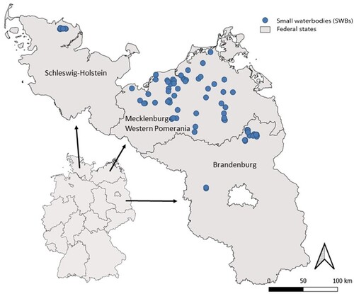
We define an SWB as having a maximum water surface extent of 1 ha (0.01 km²; Glandt 2006, Biggs et al. 2007, Ulrich et al. 2022). The sampled waterbodies are located in the young moraine landscape of the northeastern German lowlands (Fig. 1), a region containing >150 000 so called “kettle holes” that cover up to 5% of the agricultural area (Kalettka and Rudat 2006, Pätzig et al. 2012). Kettle holes represent SWBs. These small, isolated, depressional wetlands formed during the last glacial period are heterogeneous, with a high potential for biological species diversity (Kalettka and Rudat 2006). Some SWBs undergo wet/dry cycles and, because of their size, are susceptible to temperature changes and influences from their surrounding landscapes (Kalettka and Rudat 2006), such as changes in water level and nutrient loads (Lischeid et al. 2018) and pesticide contamination (Ulrich et al. 2022). These pollutants originate mainly from agricultural practices and are agricultural stressors. We sampled 100 SWBs, of which 91 were located on agriculturally arable land, mainly rapeseed and winter wheat crops, and 9 were located on nonagricultural grassland sites that could be described as meadows used extensively for pasture or feed production. Because the sampling period must occur before the merolimnic insects hatch, sampling for the north German lowlands was conducted in spring (30 March to 30 May) during 2015 to 2020 (LAWA 2021).

Figure 1. Sampling points in 3 federal states in Germany.

Field and laboratory methods for invertebrate samples

The benthic invertebrate communities were sampled manually with a hand net (mesh size 500 μm) using a habitat-specific and area-standardized method, based on the sampling regulation by Brauns et al. (2016). When present in an SWB at a proportion >5%, the sampled habitats were sand, fine particulate organic matter (FPOM), coarse particulate organic matter (CPOM), submersed macrophytes, reed, flooded terrestrial vegetation, overhanging terrestrial vegetation, stones, and dead wood. The standard sampling area used for all habitats to the greatest extend possible was 2.25 m² (3 replicates of 0.75 m² consisting of 5 hand net hoists of 0.6 m length). The dead wood and stone habitats were sampled by collecting 3–5 stones or branches (depending on size), gently brushing off attached individuals, and then measuring stone or branch area. The invertebrate samples were stored in 96% ethanol until further processing.

Before identification, all individuals were sorted into groups (Arachnida, Asellidae, Bivalvia, Chironomidae, Coleoptera, Diptera, Ephemeroptera, Gastropoda, Gammaridae, Heteroptera, Hirudinea, Lepidoptera, Megaloptera, Odonata, Oligochaeta, Plecoptera, Trichoptera, and Turbellaria). When >200 individuals from one group were present in one replicate sample, the first 200 individuals from the sample were used for the taxonomic identification, a method representative of the sample that prevents disproportionately high identification costs. Remaining organisms in the sample were then counted and allocated on a percentage basis to the numbers of identified species. Taxonomical identification was classified to the lowest taxonomic level, species level when possible (detailed description of dataset handling for different taxonomic levels discussed later).

Field and laboratory methods for water samples

Mixed water samples (∼5 L) were taken by grab sampling from about 4 to 6 locations around the shoreline of each SWB. Samples for pesticide analysis were transferred to prewashed glass bottles; bottles for pyrethroid analysis contained dichloromethane (50 mL). Water samples were analyzed using multiple methods validated for varying numbers of active substances. Because the samples were taken over a period of 5 years and the analytical methods developed over time, the number of pesticides analyzed in the samples ranged from 40 to 118 (Supplement A and B).

All pesticides in the water samples except pyrethroids, glyphosate, and aminomethylphosphonic acid (AMPA) were quantified by liquid chromatography mass spectrometry in electrospray ionization mode (LC-ESI-MS/MS) using the internal standard method after solid phase extraction (Chromabond HR-P, Macherey-Nagel, Germany, 50–100 μm particle size, 3 mL column volume, 200 mg filling quantity). From 2015 to 2018, we used an Ultimate 3000 RS (Dionex, Thermo Fisher, USA) coupled to a QTRAP 5500 mass spectrometer (AB SCIEX, USA), and in 2019 and 2020, we used a 1290 Infinity II LC system (Agilent, USA) coupled to a QTRAP 6500 + mass spectrometer (SCIEX, USA) and the previously mentioned system (LC-ESI-MS/MS). Reference standards in solvent were used. For pyrethroids, the active substances in the water sample were concentrated by liquid–liquid extraction and then analyzed by gas chromatography–mass spectrometry (GC-MS) using a Trace GC Ultra coupled to a TSQ Quantum GC XLS mass spectrometer (both from Thermo Electron Corporation, USA). Glyphosate and its metabolite AMPA were measured directly from the water samples by LC-ESI-MS/MS after derivatization with 9-fluorenylmethyl-chlorformate.

The recovery of pesticides was in the range of 0.0010–0.50 μg/L. The limits of quantification (LOQ) were active substance specific, and proprtions ranged from 0.001 to 0.0500; 0.3 μg/L (AMPA) and 0.4 μg/L (glyphosate). The limits of detection (LOD) were half the LOQs.

Samples for nutrient analysis were unfiltered (2015–2018) or filtered through a 0.45 µm cellulose acetate filter (2019 and 2020). The concentrations of NH₄⁺ and PO₄³⁻ were measured photometrically using a spectrophotometer (DR/2000 Hach) according to DIN 38 406–5 and EN ISO 6878:2004, respectively. NO₃⁻ and NO₂⁻ concentrations were analyzed by high-performance liquid chromatography (HPLC, Agilent 1100 Series HPLC System DAD, USA). The range of measurement for NH₄⁺ was 0.02–2.0 mg/L (undiluted), for PO₄³⁻ was 0.01–2.0 mg/L, and for NO₃⁻ and NO₂⁻ was 0.1–15.0 mg/L.

Physicochemical water parameters (oxygen content, electrical conductivity [EC], pH, and temperature) were measured in situ using a portable meter (WTW Multi 3430 IDS with OxiCal-SL FDO 925, TetraCon 925, and SenTix 940 probes, Germany).

Dataset

The dataset contained abundance data for the following groups of benthic invertebrates: (1) family Hydrachnidae; (2) orders Coleoptera, Diptera, Ephemeroptera, Heteroptera, Lepidoptera, Megaloptera, Odonata, Oligochaeta, and Trichoptera; (3) subclasses Hirudinea and Oligochaeta; (4) classes Bivalvia, Gastropoda, and Turbellaria; and (5) subphylum Crustacea.

It also contained data on the following environmental parameters: pH, temperature, EC, oxygen content, land use (agricultural or grassland), day of the year (DOY) of sampling, NO₃⁻ concentration, NH₄⁺ concentration, PO₄³⁻ concentration, maximum toxic units (TU_max) for pesticides, and the number of habitats sampled in the waterbody (1–4).

Data preparation and analysis

Taxonomic adjustment

Different basic methods used to resolve invertebrate datasets with various taxonomic levels are described by Cuffney et al. (2007). For the present dataset, we applied the method of distributing parents (higher taxonomic level) among children (lower taxonomic level) with the variant of adding parents abundances proportionally to each child abundance in the sample (DPAC-S) and the method to merge children with parent (MCWP-S) by adding children abundances to parent abundances per sample (Cuffney et al. 2007).

First, the mean abundance per m² per order/genus/family/species was calculated from the community abundance data. Taxonomic adjustment was performed to the lowest taxonomic level possible to prevent inconsistencies that could bias the statistical analysis (e.g., overlapping of taxa or differences in the taxonomic determination level between samples; Supplement C). When data were adjusted to a lower taxonomic level (e.g., from Pisidium sp. to P. milium and P. obtusale) the abundances were assigned on a percentage basis according to the occurrence in the sample (DPAC-S). When data were adjusted to a higher taxonomic level, the lower-level abundances were added to the higher level (e.g., the Cataclysta lemnata was resolved and abundance was added to that of Cataclysta sp.; MCWP-S). In some cases, the occurrence of taxa in neighboring waterbodies or repeated samples was used for the adjustment.

Toxicity calculations

To summarize the toxic pressure represented by each sample, TU_max (equation 1), values were calculated for the pesticide concentrations based on half maximal effective concentration (EC₅₀) or 50% lethal concentration (LC₅₀) values for invertebrates. The EC₅₀ is the acute 48 h concentration having an effect (immobilization) on 50% of test organisms, and the LC₅₀ is the acute 96 h concentration lethal for 50% of test organisms. Each measured pesticide concentration was divided by the effective concentration for the most sensitive test organism (Daphnia magna or Chironomus sp.), obtained from the Pesticides Properties Database (Lewis et al. 2016) or Ecotox Database (Olker et al. 2022) (Supplement D): (1) $\mathrm{T}{\mathrm{U}}_{\max }=\log \underset{\mathrm{i}=1}{\overset{\mathrm{n}}{max}}\left({\displaystyle \frac{\mathrm{Ci}}{\mathrm{E}{\mathrm{C}}_{{50}_{\mathrm{i}}}/\mathrm{L}{\mathrm{C}}_{{50}_{\mathrm{i}}}}}\right),$(1) where C_i is the concentration of pesticide i in μg/L. Concentrations below the LOQ but above 0 were replaced with half of the LOQ.

Data transformation and standardization

The community dataset was Hellinger transformed to reduce the effects of high abundances. Additionally, a second community dataset transformed according to variable presence/absence was created. The right-skewed explanatory variables EC and NO₃⁻, NH₄⁺, and PO₄³⁻ concentrations were log transformed before standardization. NO₃⁻, NH₄⁺, and PO₄³⁻ concentrations, TU_max, temperature, EC, pH, and O₂ content parameters were z standardized (scale function, base package; R Core Team 2022). Land use and the number of habitats sampled were coded as factors.

Multivariate statistical analyses

All data processing and statistical analyses were performed with R Studio 4.2.1, (R Core Team 2022). Multivariate analyses were performed for samples with complete observations and were based on the taxonomically harmonized community dataset. Several generalized linear models (GLMs) were run, and permutational multivariate analysis of variance (PERMANOVA) and a partial redundancy analysis (pRDA) were performed.

GLMs, robust means of analyzing non-normally distributed response variables, were used to examine the influence of predictor variable sets on the following response variables: Shannon index (Shannon 1948), evenness index (Pielou 1966), number of EPT taxa (Ephemeroptera, Plecoptera, and Trichoptera taxa), overall number of taxa, and %EPT (Lenat 1988). The Shannon and evenness indices are used widely to represent biodiversity; undisturbed communities are assumed to be characterized by high diversity and an even distribution of abundance across species (Li et al. 2010). The EPT taxa index is used widely to reflect water quality because EPT taxa are sensitive to water pollution.

First, a global model was established with all parameters selected for incorporation based on data exploration and collinearity analysis where a correlation coefficient threshold of |0.7| was applied (gvif function, car package; Dormann et al. 2013, Fox and Weisberg 2019), including for the interaction terms. For all GLMs except %EPT (binomial family), the Gaussian family was used. From the global model, all possible models were computed via automated model selection (dredge function, MuMIn package; Barton 2022). For the Shannon index, evenness index, number of EPT taxa, and total number of taxa, the best subset of models (delta Akaike information criterion [ΔAIC] ≤ 2) was chosen, and model averages were calculated for parameter estimates. This approach takes model uncertainty into account and provides robust parameter estimates (Grueber et al. 2011).

To eliminate the potential overriding influence of the number of habitats and land use response variables, the dataset was further divided into arable, single-habitat, and multi-habitat sets. Thus, computations were performed with the following datasets: (1) full dataset (105 samples); (2) only SWBs on arable land (97 samples); (3) only SWBs containing a single habitat (59 samples); (4) only SWBs containing a single habitat of the type reed, macrophytes, FPOM/CPOM (56 samples); (5) only SWBs on arable land containing a single habitat of the type reed, macrophytes, FPOM/CPOM (51); (6) only SWBs on arable land containing a single habitat of the type reed, macrophytes, FPOM/CPOM, overhanging vegetation, and other (54); (7) only SWBs containing multiple habitats (46 samples); and (8) only SWBs on arable land containing multiple habitats (43 samples). The habitat type (3 or 5 categories) served as an explanatory variable in the single-habitat analyses.

PERMANOVA was carried out with the vegan package (adonis2 function; Oksanen et al. 2022) to identify variable groupings that best explained differences in community composition. PERMANOVA is a nonparametric approach analogous to univariate ANOVA that assumes the exchangeability of permutable units only under a true null hypothesis (no difference between groups; p ≤ 0.05; Anderson 2014). The selected groupings were the habitat number (single vs. multiple), land use (arable vs. grassland), toxicity (polluted vs. unpolluted according to the threshold of TU_max = –3.27; Liess et al. 2021), and habitat type (3 and 5 variable datasets).

To identify a linear combination of environmental variables that best explained the data but also depended on the species distribution and accounted for site location, pRDAs were performed with all 8 datasets. Stepwise model construction via backward selection was performed for the Hellinger- and presence/absence-transformed datasets. Significant variables (p ≤ 0.05) after backward selection, toxicity, and habitat number were included in the analyses. Latitude and longitude were included as conditioned variance. These analyses were performed using the rda and ordistep functions in vegan (Oksanen et al. 2022). The significance of models and axes was assessed using a permutation test (n = 999, p ≤ 0.05; anova.cca function, vegan package; Oksanen et al. 2022).

Results

Community composition

We collected 111 total samples: 90 SWBs were sampled once, 9 SWBs were sampled twice, and 1 SWB was sampled 3 times. In total, 407 distinct species were represented in the nonharmonized dataset (Supplement E). Most species belonged to the orders Diptera (n = 120) and Coleoptera (n = 117), followed by the order Trichoptera (n = 50). For the other groups, species numbers varied from 0 (Hydrachnidia) to 31 (Gastropoda).

The taxonomically harmonized dataset represented 185 taxa, of which 23 taxa (12.4%) occurred in 50% of the samples and 65 (35%) occurred in <5% of the samples.

In general, the samples in the nonharmonized and harmonized datasets and those from both land use categories contained a broad range of taxa (Table 1). The range for the grassland dataset was smaller. Additionally, the variance around the mean values for EPT taxa, Coleoptera, Odonata, and Chironomidae was large for both land use categories. Relative to the samples collected from arable sites, the grassland samples had about twice the mean number and proportion of EPT taxa, a slightly larger mean proportion of Odonata, and a smaller mean proportion of Coleoptera. The mean Shannon and mean evenness indices indicated a difference from 0.2 to no difference, respectively, between categories.

Table 1. Structural composition of communities of waterbodies in arable- and grassland-dominated fields based on 102 samples from arable land and 9 samples from grassland sites. Values in brackets indicate standard deviation. Bold = based on taxonomically harmonized dataset.

	Arable land	Grassland
Species number range	5–89	21–59
Mean number of taxa determined to species	36.8 (16.2)	40.2 (14)
Taxa range after taxonomic harmonization	3–63	21–52
Mean number of taxa	35.3 (12.2)	37.3 (9.6)
EPT-taxa range	0–13	4–14
Mean number of EPT taxa	4.9 (2.8)	10.2 (2.9)
Mean % EPT taxa	20.9 (20.8)	46.3 (24)
Mean % Coleoptera	8.5 (10.2)	3.0 (4.1)
Mean % Odonata	2.6 (3.4)	4.6 (4.5)
Mean % Chironomidae	21 (21.7)	10.9 (14.8)
Shannon index, mean values	1.9 (0.6)	2.1 (0.4)
Evenness index, mean values	0.5 (0.1)	0.6 (0.1)

The mean concentrations of agricultural stressors (nutrient concentrations) were lower for grassland than for arable sites (Table 2). The mean concentration of the toxicity is similar for grassland and arable sites. For the arable land sites, the NO₃⁻ values and EC values showed especially strong variation.

Table 2. Overview of environmental parameters and day of sampling based on 102 samples from arable land and 9 samples from grassland sites. Values in brackets indicate standard deviation.

	Arable land	Grassland
Mean number of habitats (1–4)	1.6 (0.7)	1.3 (0.5)
Mean toxicity (TUmax)	−3.6 (1.7)	−3.7 (1.3)
Mean ammonium (NH4^+) [mg N/L]	0.3 (0.7)	0.1 (0.2)
Mean nitrate (NO3^−) [mg N/L]	5.5 (12.1)	0.1 (0.0)
Mean phosphate (PO4^3−) [mg P/L]	0.6 (1.1)	0.1 (0.1)
Mean pH	8.0 (0.7)	8.1 (0.4)
Mean temperature [°C]	14.0 (4.6)	10.1 (1.9)
Mean oxygen content [mg/L]	10.5 (2.7)	10.5 (3.2)
Mean EC (electronic conductivity) [µS/cm]	582.8 (456.0)	394.1 (191.3)
DOY (day of the year of sampling)	115.3 (15.4)	110.4 (12.3)

GLMs

For the full dataset (105 samples from 94 SWBs with complete data), the number of habitats contributed significantly to the Shannon index and number of taxa (Table 3). Land use significantly contributed to the number of EPT taxa (p < 0.0001). For all datasets, the DOY was a significant explanatory variable for the number of taxa (Table 3).

Table 3. Results for the model-averaged coefficients (full average) of the GLMs. Significant p values are given for the variables. Significant interaction terms are listed in the last column with their respective p value. For all response variables a Gaussian family link was used. n = number of samples in the dataset, DOY is day of year, T is temperature, EC is electrical conductivity.

	No. of habitats	Habitat type	Land use	DOY	Toxicity	NH4^+	NO3^−	PO4^3−	pH	T	O2	EC	Interaction terms
Shannon-index (n = 105)	0.0625 (hab_2)	NA	—	—	—	—	—	—	—	—	—	—	—
Single-habitat (n = 59)	NA	—	—	0.00759	—	0.03882	—	0.02223	—	0.04365	—	—	0.00222 (NH4^+:NO3^−) 0.00266 (NH4^+:PO4^3-) 0.01178 (NH4^+:toxicity) 0.00604 (NO3^−:toxicity) 0.00518 (NH4^+:NO3^−:PO4^3−)
Multi-habitat (n = 46)	NA	NA	—	—	—	—	—	—	—	—	—	—	—
arable-single-habitat types (3) (n = 51)	NA	2.01x10^-5 (macrophytes) 9.60x10^-6 (reed)	NA	0.01936	—	—	—	0.00690	—	0.03761	—	0.03299	0.03399 (NO3^−:toxicity) 0.02188 (PO4^3−:toxicity) 0.00632 (NH4^+:NO3^−:PO4^3-)
Single-habitat types (3) (n = 56)	NA	0.000116 (macrophytes); 5.3x10^-6 (reed)	—	—	—	0.025529	—	—	—	0.045633	—	—	0.002740 (NH4^+:NO3^−) 0.015535 (NH4^+:PO4^3−) 0.018133 (NH4^+:toxicity)
Evenness-index (n = 105)	—	NA	—	—	—	—	—	—	0.03815	—	—	0.00493	0.00705 (NH4^+:NO3^−:toxicity)
EPT taxa (n = 105)	—	NA	4x10^-7	0.02579	0.00255	—	—	—	—	0.0022	—	—	—
arable (n = 97)	—	NA	NA	—	0.00474	—	—	—	—	0.00399	—	—	—
Taxa number (n = 105)	5.2x10^-6 (hab_2) 0.002110 (hab_3) 6.9x10^-6 (hab_4)	NA		0.000152	—	—	—	—	—	—	—	—	—
Arable land (n = 97)	2.4x10^-6 (hab_2) 0.000929 (hab_3) 8.5x10^-6 (hab_4)	NA	NA	0.000308	—	—	—	—	—	—	—	—	—
Single-habitat arable (n = 54)	NA	—	NA	0.00471	—	—	—	—	—	—	—	—	—
Multi-habitat arable (n = 43)	NA	NA	NA	2.12x10^-5	—	—	—	—	—	—	—	—	—
Single-habitat (n = 59)	NA	—	—	0.00095	—	—	—	—	—	—	—	—	—
Single-habitat types reduced (n = 56)	NA	0.00216 (macrophytes); 4.4x10^-6 (reed)	—	0.00182	—	—	—	—	—	—	—	—	—
Multi-habitat (n = 46)	NA	NA	—	3.45x10^-5	—	—	—	—	—	—	—	—	—

For single habitats (56 samples), the habitat type (n = 3) was a significant explanatory variable for the Shannon index (habitat type macrophytes p < 0.0001 and habitat type reed p < 0.0001) and overall number of taxa (habitat type macrophytes p < 0.01 and habitat type reed p < 0.0001). The PO₄³⁻ concentration was a significant explanatory variable for the Shannon index for single habitat samples (n = 59) and for single-habitat SWBs on arable land (n = 3 habitat types; 50 samples, p < 0.05). For the response variable number of EPT taxa (full dataset, 103 samples), the toxicity was a significant explanatory variable (p < 0.05). Agricultural stressors contributed to the explanation of the Shannon-index in three of the five subsets. However, interaction terms with combinations of the variables NO₃⁻, NH₄⁺, PO₄³⁻, and toxicity significantly explained responses in 4 models run with the full datasets (105 samples) for subsets of data for the Shannon index, evenness index, and number of taxa (Table 3).

PERMANOVA

The null hypothesis, that no differences exist between the groups, can be rejected on a 95% confidence interval for the variables land use, sampling and habitat type. Group differences were more pronounced for the habitat type than for the, sampling time, land use, and habitat number. For the Hellinger-transformed and presence/absence single-habitat split sets, the habitat type explained 10.5–15.7% and 8.9–15.9%, respectively, of community differences (Table 4).

For the presence/absence community dataset, the top 5 taxa per group contributing most to differences among the 7 groups examined comprised 24 taxa from 8 orders, primarily Coleoptera (46%) and Trichoptera (20%; Table 5).

Table 4. Results of the PERMANOVA run separately for the grouping variables. The values give the difference between the groups in percent. Values in brackets are the p values. n = number of samples in the dataset. Five habitat types^† (CPOM, FPOM, reed, macrophytes, and others; 3 habitat types^‡ (CPOM/FPOM, reed, macrophytes).

	Habitat (single/ multi)	Land use (arable/ grassland)	Sampling (early/late)	Toxicity (polluted/ less polluted)	Habitat type (5^† or 3^‡)
Hellinger-transformed community data (n = 105)	1.6 (0.051)	3.0 (0.001)	3.5 (0.001)	1.5 (0.0049)	NA
Single-habitat (n = 59)^†	NA	3.4 (0.008)	4.0 (0.005)	2.6 (0.078)	13.7 (0.001)
Arable, single-habitat (n = 54)^†	NA	NA	4.6 (0.002)	3.0 (0.055)	15.7 (0.001)
Arable, single-habitat (n = 51)‡	NA	NA	5.0 (0.006)	3.0 (0.068)	10.5 (0.001)
Multi-habitat (n = 46)	NA	5.6 (0.001)	4.5 (0.003)	3.7 (0.028)	NA
Presence-absence transformed community data (n = 105)	1.9 (0.008)	4.1 (0.001)	3.9 (0.001)	1.9 (0.018)	NA
Single-habitat (n = 59)^†	NA	5.1 (0.001)	4.1 (0.002)	2.8 (0.052)	13.7 (0.002)
Arable, single-habitat (n = 54)^†	NA	NA	5.0 (0.001)	3.1 (0.046)	15.9 (0.001)
Arable, single-habitat (n = 51)^‡	NA	NA	5.4 (0.001)	4.3 (0.007)	8.9 (0.001)
Multi-habitat (n = 46)	NA	5.3 (0.007)	5.9 (0.001)	3.4 (0.073)	NA

Table 5. Contributions of species to differences between groups. For each dataset and variable, the first 5 species are shown with their respective contribution (averages) to the group differences. Values are given in percent. Calculated using the simper function, vegan package in R (Oksanen et al., 2022). Community data for this analysis was presence–absence transformed.

	Full dataset (n = 105)				Arable, single-habitat samples, habitat type (n = 51)
	Habitat (single/ multi)	Land use (arable/ grassland)	Sampling (early/late)	Toxicity (polluted/less polluted)	Reed vs. macro-phytes	Reed vs. CPOM/FPOM	Macro-phytes vs. CPOM/FPOM
Caenis horaria		1.206
Athripsodes aterrimus		1.103
Hippeutis sp.		0.955
Triaenodes bicolor		0.95
Oectis furva		0.884
Hygrotus sp.	0.799		0.755
Hydroporus sp.	0.779
Cataclysta sp.	0.741
Dytiscinae Gen. sp.	0.729		0.786	0.748
Agabus sp.	0.729
Asellidae Gen. sp.			0.77	0.789		1.22
Limnephilus flavicornis			0.801			1.264
Hydrobius sp.			0.839	0.784
Corduliidae/Libelluidae Gen. sp.	0.733			0.768
Segmentina sp.				0.745	0.919
Culicidae Gen. sp.						1.33	1.351
Scirtidae Gen. sp.						1199
Limoniidae Gen. sp.						1.203
Limnephilus vittatus					0.947		1.364
Helochares sp.					0.95
Anacaena sp.					0.939
Stratiomyidae Gen. sp.							1.397
Enochrus sp.					0.97		1.621
Colymbetinae Gen. sp.							1.241

Table 6. Results from the pRDA. Latitude and Longitude used as input for the conditioned variance. Variable outcome from the backward selection of the RDA plus toxicity and number of habitats. Hellinger-transformed dataset used. n = number of samples in the dataset.

	Significant variables after backward selection + toxicity + habitat number	Conditioned variance explained in %	Constrained variance explained in %	Adjusted R^2 of constrained variance explained in %
Complete dataset (n = 105)	PO4^3− + EC + pH + land use + DOY + toxicity + habitat number	3.1	15.8	8.1
single-habitat SWBs (n = 59)	EC + pH + DOY + habitat type + toxicity	3.5	23.3	11.5
single-habitat SWBs reduced (grouped to three habitats (n = 56)	EC + pH + DOY + habitat type + toxicity	9.1	21.3	12.9
multi-habitat SWBs (n = 46)	NO3^− + DOY + toxicity + habitat number	5.8	18.1	6.0
Arable land (n = 97)	EC + pH + DOY + toxicity + habitat number	3.5	12.4	5.8
single-habitat SWBs (n  =54)	EC + pH + DOY+ habitat type + toxicity	4.0	25.1	12.4
single-habitat SWBs (n = 51 with grouped [3 groups] habitat type as parameter)	EC + pH + DOY+ habitat type + toxicity	4.3	23.1	13.2
multi-habitat SWBs (n = 43)	NO3^− + DOY + toxicity + habitat number	6.3	13.7	2.5

We report results for the Hellinger transformed dataset. The DOY was a significant variable in all models (Table 6). Six of eight models showed significant contributions of EC and ph. Nutrient concentrations were significant variables in three models. The location (conditioned variance) explained 3.1–9.1% of the variance (Table 6). Adjusted R² values indicated that 2.5–13.2% of the variance in these respective datasets was explained by constrained variance (Table 6). In general, the tested variables performed better in explaining the data for single-habitat SWBs.

The pRDA (Fig. 2) given for the first 2 axes shows the relationships between species and the significant environmental variables (pH, EC, DOY, habitat type; p < 0.05) and toxicity. Only species that explained at least 25% of the variability are shown. DOY, toxicity, and EC are mostly related to waterbodies with the habitats macrophytes and reed, with a stronger association to the macrophyte cluster. The colored polygons depicted for the 3 habitat types show a clustering of communities in habitat types, but strong overlaps are observed for the communities in SWBs with only macrophyte habitats present.

Figure 2. Ordination diagram of first 2-axis pRDA analysis based on the Hellinger-transformed abundance data, conditioned for spatial variation. Environmental parameters with continuous values (DOY, toxicity, EC, pH) are shown as blue arrows. Environmental parameter habitat described as a factor is shown as colored polygons. Species that explain at least 25% of variation are shown as black arrows. Gen. sp. denotes grouping that includes genera/species

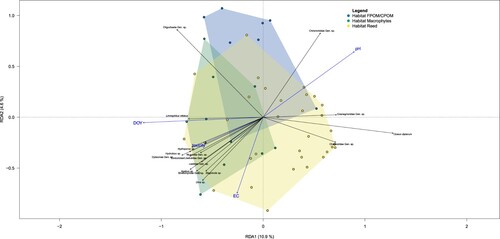
The family Chironomidae and the subclass Oligochaeta are closely assigned to FPOM/CPOM habitats, and the species Cloeon dipterum and the families Coenagrioniidae and Chaoboridae are closely assigned to the reed habitat. Taxa positively associated with the habitats reed and macrophytes are, with 4 exceptions, predators, and 4 of 11 taxa are from the order Coleoptera, strongly associated with vegetated habitats. The pRDA reflects the results from the contribution of habitat type to the group differences of the PERMANOVA.

Discussion

In this study, we examined the structural composition and response of benthic invertebrate communities in SWBs to agricultural stressors in a lowland area of northeast Germany with strong agricultural influence.

We obtained 3 main results. First, benthic invertebrate communities in SWBs have a diverse taxon composition; 35% of taxa were found in <5% of samples. Second, the structural diversity indicators examined did not respond to agricultural stressors. Third, the habitat number and type (only for single-habitat samples) performed best in explaining community compositions.

The taxonomic diversity of community compositions is in line with previous findings (Williams et al. 2003, Kelly-Quinn et al. 2017) and emphasizes the importance of every SWB for the promotion and conservation of freshwater invertebrate biodiversity. Scheffer et al. (2006) observed high beta diversity of benthic invertebrates in small lakes and ponds, which can be explained by the unique micro-site conditions, habitat features, and isolation of SWBs. Additionally, random processes in community dynamics could have led to idiosyncratic distribution patterns (Briers and Biggs 2003). Onandia et al. (2021) and Briers and Biggs (2003) found diverse community compositions among SWBs, with 30% of rotifer genera recorded in a single waterbody (Onandia et al. 2021) and, on average, <20% of benthic invertebrate species shared between ponds (Briers and Biggs 2003). These results are in line with the first finding that the invertebrate community strongly differs among the SWBs. Therefore, we assume that explanations such as habitat features, isolation of waterbodies, or idiosyncratic distribution patterns may also be key drivers in SWBs.

An unexpected finding of the study was the poor performance of the Shannon and evenness indices, and overall taxa in detecting agricultural stressor impacts in the multivariate analyses. Our hypothesis that species richness would decrease and the number of tolerant taxa would increase in benthic invertebrate communities under this type of stress was not confirmed, which can be explained only partially by the timing of sampling. Because chemical and biological sampling were performed in parallel, possible peak concentrations (e.g., due to runoff events) of pesticide residues and nutrient concentrations may have been undetected. Widespread eutrophication due to intensive agriculture has been shown to override the local effects of land use on rotifer (Onandia et al. 2021) and benthic invertebrate (Krynak and Yates 2018) communities. Thus, we assume the poor response to agricultural stressors in this study was due to the long-term and ubiquitous occurrence of the stressors in the landscapes examined. As a result, short gradients of stressors were acting in the studied SWBs, hampering the identification of responses to agricultural stressors using structural community composition measures. This assumption is supported by the Krynak and Yates (2018) finding that habitat variables better predict taxon abundance (at the family and genus levels) and functional trait compositions than does agricultural activity.

Furthermore, the identification of causal relationships between pesticide contamination and the response of invertebrate communities is challenging in field studies (Beketov and Liess 2012). Additional factors such as landscape characteristics (e.g., refugia; Brock et al. 2010), variability over time and space, and the idiosyncratic responses of individual taxa to environmental factors (Jeffries 2003) contribute to community composition. We assume these factors also led to the poor performance of the indicators in this study. We observed a trend towards larger numbers of taxa in late sampling periods. Presumably, individuals were larger and could be sampled and identified more easily during this period, as reflected by the influence of the DOY on the number of taxa but no other indicators in the GLMs, and by significance of the DOY for model selection in the pRDAs.

Liess et al. (2021) concluded that pesticides are the dominant stressors for vulnerable aquatic insects; however, they sampled invertebrates in small streams later in the year (at the beginning of June), which could mean that some vulnerable taxa had already emerged from the waterbodies. Furthermore, they performed automated event-driven water sampling and sampling at 3-week intervals during the pesticide application period (Liess et al. 2021), which is a targeted approach to the demonstration of the likely function of pesticides as main stressors. Nevertheless, in line with our findings, they found that common biodiversity indices were associated only weakly with anthropogenic stressors (Liess et al. 2021). The functional SPEAR_Pesticides index best reflected the effects of these stressors in their study (Liess et al. 2021). Although the SPEAR_Pesticides index was developed for running waters, we tested a functional GLM-based approach with using the SPEAR_Pesticides index as well as the saprobic index serving as response variables (results not shown). In our model for the SPEAR_Pesticides index the pesticide toxicity, PO₄³⁻ concentration, and DOY were significant explanatory variables. With the saprobic index serving as a response variable, the pH, was a significant explanatory variable. Therefore, we suggest that future studies on agricultural impacts on benthic invertebrates in SWBs should focus on functional responses rather than on structural metrics. Functional metrics enable the comparison of community compositions at a broader spatial scale and diversity patterns in regions in which communities are composed of different taxa (Múrria et al. 2020).

We found that the habitat factor had more explanatory power than did agricultural stressors. For the Shannon index and number of taxa, the habitat type was the dominant factor influencing community compositions in single-habitat samples. This factor also explained 2–3 times more of the difference in community composition than did toxicity in the Hellinger-transformed and presence/absence single-habitat arable-land datasets.

Limnephilus vittatus, a habitat specialist (phytal), contributed to group differences among 3 habitat types. Two other habitat specialists (Athripsodes aterrimus [psammopelal] and Triaenodes bicolor [phytal]) contributed to group differences between arable land and grassland. The fourth habitat specialist (Cataclysta sp. [phytal]) contributed to differences between multi-habitat and single-habitat groups.

The pRDA conducted in this study explained more variance for single-habitat SWB models than for other models. The models performed better when the habitat type was incorporated and clusters by habitat types were observed. We assume that habitat filtering is responsible for the power of this variable in explaining community composition, as shown for the composition of stream insect communities (Smith et al. 2015).

Conclusion

This study showed that (1) the benthic invertebrate communities in the examined SWBs are highly diverse; (2) the structural diversity indicators examined do not respond to agricultural stressors in SWBs as expected; and (3) habitat number and type (for single-habitat samples) performed best in explaining community compositions in SWBs.

Those findings suggest that direct agricultural stressors play minor roles in structuring benthic invertebrate composition in SWBs. However, eutrophication and pesticides can have indirect effects on benthic invertebrate communities. Those indirect effects, such as influences of herbicides on macrophyte communities and thus on habitat structures, could not be examined in this study. In a descriptive overview of nutrient concentrations, we found an influence of land use on the variable. We observed lower nutrient concentrations in water samples from grassland sites. Nevertheless, more sensitive indices and test functional metrics are needed as biological indicators for the effects for agricultural stress on benthic invertebrates in SWBs. The existing functional metrics to detect effects of water pollution on invertebrate communities, such as the SPEAR_Pesticides index (Liess and Ohe 2005), are designed for application to flowing waters and thus are not applicable for SWBs. Hence, we suggest testing functional indicators and examining possible indirect effects to detect stressed or disturbed communities, specifically in SWBs.

Author contribution statement

Conceptualization: FNT, SL. Developing methods: FNT, KF, SL. Data analysis: FNT. Conducting the research: FNT, KF, SL. Data interpretation: FNT, SL. Preparation of figures and tables: FNT.

Acknowledgements

The authors thank Anne Köppen, Manuel König, Agnes Teuber, and Elke Zeidler for their assistance during field sampling campaigns. Furthermore, we thank Dominique Conrad, Michael Glitschka, Christine Reichmann, Ina Stachewicz, and Gabrielle Smykalla for their help in sample preparation and pesticide and nutrient analysis. In addition, we thank Anne Köppen, Manuel König, Jörg Stauch, Agnes Teuber, Elke Zeidler, and the commissioned entomologists for the preparation and determination of the biological samples. Thanks also to Matthias Stähler for sample analysis and discussions on analytical methods during the paper writing process.

Disclosure statement

No potential conflict of interest was reported by the author(s).

Data availability statement

Due to the sensitive nature of the questions asked in this study, farmers were assured raw data would remain confidential and would not be shared, and respondents would not be identified individually. All data on the analytical methods can be requested from the authors.

Correction Statement

This article has been corrected with minor changes. These changes do not impact the academic content of the article.

Additional information

Funding

During this work, FT received funding from the Fachagentur Nachwachsende Rohstoffe e.V. (FNR) under grant 22012118, 2221NR094B 8.

References

- Anderson MJ. 2014. Permutational multivariate analysis of variance (PERMANOVA). In: Balakrishnan N, Colton T, Everitt B, Piegorsch W, Ruggeri F, Teugels JL, editors. New York (NY): Wiley StatsRef: Stats Ref Online. 48. p. 1–15.
- Barton K. 2022. MuMIn: Multi-model inference. R package version 1.46.0. https://cran.r-project.org/package = MuMIn
- Beketov MA, Liess M. 2012. Ecotoxicology and macroecology –time for integration. Environ Pollut. 162:247–254.
- Biggs J, von Fumetti S, Kelly-Quinn M. 2017. The importance of small waterbodies for biodiversity and ecosystem services: implications for policy makers. Hydrobiologia. 793:3–39.
- Biggs J, Williams P, Whitfield M, Nicolet P, Brown C, Hollis J, Arnold D, Pepper T. 2007. The freshwater biota of British agricultural landscapes and their sensitivity to pesticides. Agric Ecosyst Environ. 122(2):137–148.
- Brauns M, Miler O, Garcia X-F, Pusch M. 2016. Vorschrift für die standardisierte probenahme des biologischen qualitätselementes "makrozoobenthos" im eulitoral von seen. Leibniz-Institut für Gewässerökologie und Binnenfischerei [Regulation for the standardized sampling of the biological quality element “macrozoobenthos” in the littoral of lakes. Leibniz Institute for Freshwater Ecology and Inland Fisheries]. German.
- Briers RA, Biggs J. 2003. Indicator taxa for the conservation of pond invertebrate diversity. Aquat Conserv: Mar Freshw. 13(4):323–330.
- Brock TC, Belgers JDM, Roessink I, Cuppen JG, Maund SJ. 2010. Macroinvertebrate responses to insecticide application between sprayed and adjacent nonsprayed ditch sections of different sizes. Environ Toxicol Chem. 29(9):1994–2008.
- Céréghino R, Boix D, Cauchie H-M, Martens K, Oertli B. 2014. The ecological role of ponds in a changing world. Hydrobiologia. 723:1–6.
- Cuffney TF, Bilger MD, Haigler AM. 2007. Ambiguous taxa: effects on the characterization and interpretation of invertebrate assemblages. J North Am Benthol Soc. 26(2):286–307.
- Darwall W, Bremerich V, Wever Ad, Dell AI, Freyhof J, Gessner MO, Grossart H-P, Harrison I, Irvine K, Jähnig SC, et al. 2018. The alliance for freshwater life: a global call to unite efforts for freshwater biodiversity science and conservation. Aquatic Conserv: Mar Freshw. 28(4):1015–1022.
- Davies BR, Biggs J, Williams PJ, Lee JT, Thompson S. 2008. A comparison of the catchment sizes of rivers, streams, ponds, ditches and lakes: implications for protecting aquatic biodiversity in an agricultural landscape. Hydrobiologia. 597:7–17.
- Dormann CF, Elith J, Bacher S, Buchmann C, Carl G, Carré G, Marquéz JRG, Gruber B, Lafourcade B, Leitão PJ, et al. 2013. Collinearity: a review of methods to deal with it and a simulation study evaluating their performance. Ecography. 36(1):27–46.
- Downing JA. 2010. Emerging global role of small lakes and ponds: little things mean a lot. Limnetica. 29(1):9–24.
- Downing JA, Prairie YT, Cole JJ, Duarte CM, Tranvik LJ, Striegl RG, McDowell WH, Kortelainen P, Caraco NF, Melack JM, et al. 2006. The global abundance and size distribution of lakes, ponds, and impoundments. Limnol Oceanogr. 51(5):2388–2397.
- Dudgeon D, Arthington AH, Gessner MO, Kawabata Z-I, Knowler DJ, Lévêque C, Naiman RJ, Prieur-Richard A-H, Soto D, Stiassny MLJ, et al. 2006. Freshwater biodiversity: importance, threats, status and conservation challenges. Biol Rev Camb Philos Soc. 81(2):163–182.
- Fox J, Weisberg S. 2019. An R companion to applied regression, 3rd ed. Thousand Oaks (CA): Sage.
- Glandt D. 2006. Praktische Kleingewässerkunde. 1. Aufl. [Practical small waterbody science. 1st ed.] Laurenti: Bielefeld. Zeitschrift für Feldherpetologie [J Field Herpetol], Supplement; Vol. 9.
- Grueber CE, Nakagawa S, Laws RJ, Jamieson IG. 2011. Multimodel inference in ecology and evolution: challenges and solutions. J Evol Biol. 24(4):699–711.
- Jeffries MJ. 2003. Idiosyncratic relationships between pond invertebrates and environmental, temporal and patch-specific predictors of incidence. Ecography. 26(3):311–324.
- Kalettka T, Rudat C. 2006. Hydrogeomorphic types of glacially created kettle holes in north-east Germany. Limnologica. 36(1):54–64.
- Kelly-Quinn M, Biggs J, Fumetti Sv. 2017. Preface: the importance of small water bodies. Hydrobiologia. 793:1–2.
- Krynak EM, Yates AG. 2018. Benthic invertebrate taxonomic and trait associations with land use in an intensively managed watershed: implications for indicator identification. Ecol Indic. 93:1050–1059.
- LAWA. 2021. Rahmenkonzeption monitoring Teil B: Bewertungsgrundlagen und methodenbeschreibungen. Arbeitspapier III. Untersuchungsverfahren für biologische qualitätskomponenten. Berlin:Bund/Länder-Arbeitsgeme-inschaft Wasser (LAWA) [Framework concept monitoring Part B: evaluation bases and method descriptions. Working Paper III, Test procedures for biological quality components. Berlin: Federal/state working group on water (LAWA)].
- Lenat DR. 1988. Water quality assessment of streams using a qualitative collection method for benthic macroinvertebrates. J North Am Benthol Soc. 7(2):222–233.
- Lewis KA, Tzilivakis J, Warner DJ, Green A. 2016. An international database for pesticide risk assessments and management. Hum Ecol Risk Assess. 22(4):1050–1064.
- Li L, Zheng B, Liu L. 2010. Biomonitoring and bioindicators used for river ecosystems: definitions, approaches and trends. Procedia Environ Sci. 2:1510–1524.
- Liess M, Liebmann L, Vormeier P, Weisner O, Altenburger R, Borchardt D, Brack W, Chatzinotas A, Escher B, Foit K, et al. 2021. Pesticides are the dominant stressors for vulnerable insects in lowland streams. Water Res. 201:117262.
- Liess M, Ohe Pvd. 2005. Analyzing effects of pesticides on invertebrate communities in streams. Environ Toxicol Chem. 24(4):954–965.
- Lischeid G, Kalettka T, Holländer M, Steidl J, Merz C, Dannowski R, Hohenbrink T, Lehr C, Onandia G, Reverey F, et al. 2018. Natural ponds in an agricultural landscape: external drivers, internal processes, and the role of the terrestrial–aquatic interface. Limnologica. 68:5–16.
- Lorenz S, Rasmussen JJ, Süß A, Kalettka T, Golla B, Horney P, Stähler M, Hommel B, Schäfer RB. 2017. Specifics and challenges of assessing exposure and effects of pesticides in small water bodies. Hydrobiologia. 793(1):213–224.
- Mittermeier RA, Farrel TA, Harrison I, Upgren Amy J, Brooks TM. 2010. Fresh water: the essence of life (CEMEX conservation book series, band 18). Arlington (VA): Conservation International, USA.
- Mullins ML, Doyle RD. 2019. Big things come in small packages: Why limnologists should care about small ponds. Acta Limnol Bras. 31:181.
- Múrria C, Iturrarte G, Gutiérrez-Cánovas G. 2020. A trait space at an overarching scale yields more conclusive macroecological patterns of functional diversity. Global Ecol Biogeogr. 29(10):1729–1742.
- Oertli B, Joye DA, Castella E, Juge R, Cambin D, Lachavanne J-B. 2002. Does size matter? The relationship between pond area and biodiversity. Biol Conserv. 104(1):59–70.
- Oksanen J, Simpson G, Blanchet F, Kindt R, Legendre P, Minchin P, O'Hara R, Solymos P, Stevens M, Szoecs E, et al. 2022. vegan: community ecology package. R Package Version. 2:6–2. https://cran.r-project.org/package = vegan
- Olker JH, Elonen CM, Pilli A, Anderson A, Kinziger B, Erickson S, Skopinski M, Pomplun A, LaLone CA, Russom CL, et al. 2022. The ECOTOXicology knowledgebase: a curated database of ecologically relevant toxicity tests to support environmental research and risk assessment. Environ Toxicol Chem. 41(6):1520–1539.
- Onandia G, Maassen S, Musseau CL, Berger SA, Olmo C, Jeschke JM, Lischeid G. 2021. Key drivers structuring rotifer communities in ponds: insights into an agricultural landscape. J Plankton Res. 43(3):396–412.
- Pätzig M, Kalettka T, Glemnitz M, Berger G. 2012. What governs macrophyte species richness in kettle hole types? A case study from northeast Germany. Limnologica. 42(4):340–354.
- Pielou EC. 1966. The measurement of diversity in different types of biological collections. J Theor Biol. 13:131–144.
- R Core Team. 2022. R: a language and environment for statistical computing. Vienna (Austria): R Foundation for Statistical Computing. https://www.r-project.org/
- Reid AJ, Carlson AK, Creed IF, Eliason EJ, Gell PA, Johnson PTJ, Kidd KA, MacCormack TJ, Olden JD, Ormerod SJ, et al. 2019. Emerging threats and persistent conservation challenges for freshwater biodiversity. Biol Rev Camb Philos Soc. 94(3):849–873.
- Rolauffs P, Stubauer I, Moog O, Zahrádková S, Brabec K. 2004. Integration of the saprobic system into the European Union Water Framework Directive. In: Hering D, Verdonschot PFM, Moog O, Sandin L, editors. Chapter 17: Integrated assessment of running waters in Europe. Dordrecht: Springer Netherlands; p. 285–298.
- Savić B, Evgrafova A, Donmez C, Vasić F, Glemnitz M, Paul C. 2021. Assessing the role of kettle holes for providing and connecting amphibian habitats in agricultural landscapes. Land. 10(7):692–713.
- Schäfer RB, van den Brink PJ, Liess M. 2011. Impacts of pesticides on freshwater ecosystems. In: Sánchez-Bayo F, van den Brink JP, Mann RM, editors. Chapter 6, Ecological impacts of toxic chemicals. Soest (Netherlands): Bentham Science Publishers; p. 111–137.
- Scheffer M, van Geest GJ, Zimmer K, Jeppesen E, Søndergaard M, Butler MG, Hanson MA, Declerck S, De Meester L. 2006. Small habitat size and isolation can promote species richness: second-order effects on biodiversity in shallow lakes and ponds. Oikos. 112(1):227–231.
- Shannon CE. 1948. A mathematical theory of communication. Bell Syst Tech J. 27:379–423.
- Smith RF, Venugopal PD, Baker ME, Lamp WO. 2015. Habitat filtering and adult dispersal determine the taxonomic composition of stream insects in an urbanizing landscape. Freshw Biol. 60(9):1740–1754.
- Tews J, Brose U, Grimm V, Tielbörger K, Wichmann MC, Schwager M, Jeltsch F. 2004. Animal species diversity driven by habitat heterogeneity/diversity: the importance of keystone structures. J Biogeogr. 31(1):79–92.
- Ulrich U, Lorenz S, Hörmann G, Stähler M, Neubauer L, Fohrer N. 2022. Multiple pesticides in lentic small water bodies: exposure, ecotoxicological risk, and contamination origin. Sci Total Environ. 816:151504.
- Wagner DL. 2020. Insect declines in the Anthropocene. Annu Rev Entomol. 65:457–480.
- Williams P, Whitfield M, Biggs J, Bray S, Fox G, Nicolet P, Sear D. 2003. Comparative biodiversity of rivers, streams, ditches and ponds in an agricultural landscape in Southern England. Biol Conserv. 115(2):329–341.