Velocity tracking controller for simulation analysis of underwater vehicle model

ABSTRACT

A method for dynamics analysis of underwater vehicles is presented in this paper. The strategy consists of two stages. At the first stage, we propose an adaptive velocity tracking controller for the vehicle. The control algorithm is expressed in terms of transformed equations of motion in which the inertia matrix is diagonal. Consequently, it takes into account the dynamics of the system and it can be applied for fully actuated systems in the presence of disturbances and uncertain dynamics. Using this controller, we are able to track the velocity, and also at the same time, to evaluate some dynamic properties of the vehicle. At the second stage, we give some procedure for the dynamics analysis. The advantage of the approach is that the algorithm serves simultaneously for control purposes and dynamics investigation. It can be done before real experiment which is always expensive and time consuming. The effectiveness of the strategy is validated via simulation on a full 6-DOFs underwater vehicle model.

1. Notation

• M $\in R^{6\times 6}$ is the inertia matrix that includes a rigid body mass matrix and an added mass matrix, and satisfies $M=M^{\mathrm{T}}>0$, and $\dot{M}=0$,

• $C\left(\nu \right)$ $\in R^{6\times 6}$ is the matrix of Coriolis and centripetal terms (that satisfies $C\left(\nu \right)=-C^{\mathrm{T}}\left(\nu \right)$, $\mathrm{\forall }\nu \in R^6$),

• $D\left(\nu \right)$ $\in R^{6\times 6}$ is the matrix of hydrodynamic damping terms ($D\left(\nu \right)>0$, $\mathrm{\forall }\nu \in R^6$, $\nu \ne 0$),

• $g\left(\eta \right)$ $\in R^6$ is the vector of gravitational and buoyancy forces and moments,

• η $\in R^6$ is the vector of positions and Euler angles, $\eta =[x,y,z,\phi ,\theta ,\psi {]}^{\mathrm{T}}$,

• ν $\in R^6$ is the vector of body-fixed linear and angular velocity components, and $\nu =[u,v,w,p,q,r{]}^{\mathrm{T}}$,

• τ $\in R^6$, $\tau =[{\tau }_X,{\tau }_Y,{\tau }_Z,{\tau }_K,{\tau }_M,{\tau }_N{]}^{\mathrm{T}}$ is the control vector,

• $J\left(\eta \right)$ $\in R^{6\times 6}$ block diagonal transformation matrix relating to the body-fixed frame to the inertial reference frame (usually the earth). The matrix $J\left(\eta \right)$ depends on the Euler angles,

• $\tilde{F}$ $\in R^6$ is the uncertainty vector (containing modelling uncertainty and unknown environmental disturbances), i.e. $\tilde{F}=[{\tilde{F}}_X,{\tilde{F}}_Y,{\tilde{F}}_Z,{\tilde{F}}_K,{\tilde{F}}_M,{\tilde{F}}_N{]}^{\mathrm{T}}$,

• N $\in R^{6\times 6}$ is a diagonal inertia matrix in terms of the GVC arising from decomposition of the matrix M,

• ϒ $\in R^{6\times 6}$ is a rates transformation matrix (upper triangular),

• ξ $\in R^6$ is the GVC vector (the vector of rates after transformation of ν),

• π $\in R^6$ is a vector of forces after velocity transformation.

2. Introduction

Autonomous underwater vehicles (AUVs) are at present used in a wide range of applications, e.g. survey and exploration of ocean environment as well as underwater resources. They are uniquely suited to accomplish missions in ocean environment which are risky as coastal and inland waters monitoring. Moreover, they are characterised by low cost in comparison with full scale and fully manned vessels. One of main motion control objectives of AUVs is trajectory tracking. Sometimes also velocity tracking control algorithms are considered. In this paper, the latter issue is developed and discussed.

For underwater vehicles, many control strategies can be found in various books, e.g. in Do and Pan (2009), Fossen (1994). Tracking control algorithms for AUVs have also been proposed in Bechlioulis et al. (2017), Chen et al. (2016), Fischer et al. (2014), Garcia-Valdovinos et al. (2014), Yan et al. (2015). In Bechlioulis et al. (2017) the control algorithm guarantees trajectory tracking with prescribed performance for underactuated vehicles. The computed-torque controller in Chen et al. (2016) is based on an adaptive fuzzy observer. The continuous robust controller given in Fischer et al. (2014) was experimentally validated for an AUV. The approach based on a second-order sliding mode control for nonlinear underwater vehicles realised in the earth-fixed frame can be found in Garcia-Valdovinos et al. (2014). The scheme accomplishes position tracking without robot dynamics, nor parameters knowledge. In Yan et al. (2015), the trajectory tracking control algorithm for an underactuated underwater vehicle is appropriate only in the horizontal plane. The above mentioned solutions serve for position trajectory tracking, whereas in this work a velocity tracking scheme is considered. There exist vehicles which models are considered as fully actuated. We can point at some works in which control strategies for underwater vehicles were given (Antonelli 2007; Donaire et al. 2017; Fischer et al. 2014; Garcia-Valdovinos et al. 2014; Kim et al. 2016; Liu et al. 2017). Six controllers realised in the earth-fixed frame have been compared with respect to their behaviour in the presence of modelling uncertainty and ocean current in Antonelli (2007). The control trajectory tracking problem (Donaire et al. 2017) is solved using the port-Hamiltonian framework. An enhanced time-delay control algorithm which realises the position control of an AUV Kim et al. (2016) is suitable practically for 3-DOFs models. The backstepping finite-time sliding mode control scheme using nonlinear disturbance observer which allows one trajectory tracking of the underwater vehicle (Liu et al. 2017) is proposed for 5-DOFs models.

Moreover, velocity tracking controllers are applied in various moving systems as marine or flying vehicles. Some examples of velocity controllers are given in Ferreira et al. (2010), where vertical and horizontal controllers were applied for MARES AUV as a part of the control system. Track velocity control of underwater mining robot was considered in Yoon et al. (2012). The gain of the proportional integral controller was designed based on the gain tuning formulas and the model parameters. The tracking control approaches for underwater vehicles based on bio-inspired neurodynamics, in which also the velocity controller is considered, have been reported in Sun et al. (2013); Zhu and Sun (2013). Both papers described different control strategies but using the sliding mode approach. However, they were applied for horizontal motion of the vehicle only.

Many adaptive control schemes for various underwater vehicles were developed. An approach using estimation of the lumped uncertainty vector together with a sliding-mode-based controller for underwater vehicles was proposed in Soylu et al. (2008) and developed (Soylu et al. 2016). In the first work, the algorithm for trajectory tracking contains an adaptive term and can be applied for 6-DOFs marine systems. The second work offers a control strategy which is effective for reduced models with 4 DOFs and the diagonal inertia matrix. Other adaptive controller for AUVs which does not require an accurate model of the vehicle and is robust to unforeseen conditions was proposed and discussed in Barbalata et al. (2015). There exists also quite different adaptive strategy for trajectory control was given in Lee and Singh (2016). The algorithm lies on the fact that the control system included an auxiliary dynamic system to counter the effect of control input saturation.

In this paper, a velocity tracking control algorithm for simulation analysis of underwater vehicles is given. The algorithm is expressed in the body-reference frame instead of using the earth-fixed frame representation as in Soylu et al. (2008). Besides, in the proposed control strategy effects of vehicle dynamics can be evaluated during motion. In the cited work, any discussion of importance of couplings for control process were omitted. The controller is expressed in terms of generalised velocity components (GVCs) and it can be applied, in general, for fully actuated 6-DOFs vehicles. It is based on a velocity transformation arising from the inertia matrix decomposition. The decomposition is crucial for this approach because the obtained matrices are included directly into the control gains. This means that the controller performance is strictly related to the dynamics of the vehicle. Also, the selection of gain matrices is based on its dynamics. One of the benefits is that the system response can be achieved quickly ensuring the velocity error convergence. However, the importance of the algorithm is twofold: to track the velocity and to obtain some information about the vehicle model. This knowledge can be used next to improve the vehicle design avoiding expensive experiments. Novelty of the approach lies on that we show a nonlinear controller that has some properties observable after the inertia matrix decomposition (without the decomposition we lost information useful for control and dynamics study). The algorithm serves for control, and at the same time, it gives an insight into the vehicle dynamics. This property distinguishes our approach to the control problem of commonly used control strategies. The stability of the vehicle dynamics under the controller is given using the Lyapunov argument. The main difference between the proposed algorithm and the other known from the literature is that we use here properties resulting from the transformed equations of motion. Both the gain matrices for velocity tracking and disturbance reduction arise from the decomposition of the inertia matrix and they are strictly related to the dynamics of the vehicle.

In Section 3, we show the transformed equations of motion. The velocity tracking control algorithm and its use for dynamics analysis is considered in Section 4. Simulation results are presented in Section 5 and some conclusions are formulated in Section 6.

3. Equations of motion with diagonal inertia matrix

The real underwater vehicle is a very complicated system and its modelling is difficult because the equations of motion are strongly nonlinear. Moreover, many physical phenomena as the propeller propulsion or hull resistance must be taken into account. These problems are described, e.g. in ABS (2006); Su et al. (2013). However, the general model can be simplified to a vehicle model useful for control purposes. Such a dynamical model of a 6-DOFs underwater vehicle is expressed in the body-fixed reference frame by, e.g. (Do and Pan 2009; Fossen 1994): (1) $M\dot{\nu }+C\left(\nu \right)\nu +D\left(\nu \right)\nu +g\left(\eta \right)+\tilde{F}=\tau ,$(1) (2) $\dot{\eta }=J\left(\eta \right)\nu ,$(2) where (1(1) $M\dot{\nu }+C\left(\nu \right)\nu +D\left(\nu \right)\nu +g\left(\eta \right)+\tilde{F}=\tau ,$(1) ) is the vehicle dynamics and (2(2) $\dot{\eta }=J\left(\eta \right)\nu ,$(2) ) is the kinematics.

Remark 3.1

The proposed decomposition of the inertia matrix M (1(1) $M\dot{\nu }+C\left(\nu \right)\nu +D\left(\nu \right)\nu +g\left(\eta \right)+\tilde{F}=\tau ,$(1) ) is possible if it is assumed that the matrix is symmetric, positive definite and their elements are known. As results from Fossen (1994) for a class of underwater vehicle models such approximation can be made. Note however that, in general components of the inertia matrix depend on geometry, fluid flow rates and other uncertainties. Additionally, the added mass coefficients are often estimated using experimental studies and empirical relations which are not quite accurate. If the vehicle moves then also external disturbances and unsteady effects occur. Because we consider the matrix M as known and constant then all other factors must be taken into account in the vector $\tilde{F}$. This vector is a model of all uncertainties and disturbances. It represents forces and torques of the phenomena that are not explicitly stated in the equations of motion. So we assume that the not-modelled dynamics and environmental factors give forces and torques which can be described by $\tilde{F}$.

In order to ensure the use of the proposed approach, we define the disturbance vector $\tilde{F}$ as follows: (3) $\tilde{F}=\mathrm{\Delta }M\dot{\nu }+\mathrm{\Delta }C\left(\nu \right)\nu +\mathrm{\Delta }D\left(\nu \right)\nu +\mathrm{\Delta }g\left(\eta \right)+\mathrm{d}\left(t\right).$(3) The matrices $\mathrm{\Delta }M$, $\mathrm{\Delta }C\left(\nu \right)$, $\mathrm{\Delta }D\left(\nu \right)$ and the vector $\mathrm{\Delta }g\left(\eta \right)$ include internal inaccuracies and other model uncertainties, whereas the vector $d\left(t\right)$ represents external disturbances.

Under the above condition, the inertia matrix M is constant, symmetric, and in general, non-diagonal, i.e. it contains off-diagonal elements. Our aim is to design a decoupled controller in the sense that each rate (quasi-velocity) is regulated separately. In order to do that, we introduce a transformation of rates, i.e.: (4) $\nu =\mathrm{{\rm Y}}\xi ,$(4) where ϒ is an upper triangular, invertible matrix with constant elements arising from a decomposition of the matrix M into three matrices, i.e. $M={\mathrm{{\rm Y}}}^{-T}N{\mathrm{{\rm Y}}}^{-1}$. The matrix N is diagonal and their elements are constant.

Thus, calculating the time derivative of ν one obtains $\dot{\nu }=\mathrm{{\rm Y}}\dot{\phantom{a}}\xi$. Taking the above into account and inserting (4(4) $\nu =\mathrm{{\rm Y}}\xi ,$(4) ) into (1(1) $M\dot{\nu }+C\left(\nu \right)\nu +D\left(\nu \right)\nu +g\left(\eta \right)+\tilde{F}=\tau ,$(1) ), and pre-multiplying both sides by ${\mathrm{{\rm Y}}}^{\mathrm{T}}$ one can write: (5) $\begin{array}{rl}& M\mathrm{{\rm Y}}\dot{\xi }+C\left(\nu \right)\mathrm{{\rm Y}}\xi +D\left(\nu \right)\mathrm{{\rm Y}}\xi +g\left(\eta \right)+\tilde{F}=\tau ,\end{array}$(5) (6) $\begin{array}{rl}& {\mathrm{{\rm Y}}}^{\mathrm{T}}M\mathrm{{\rm Y}}\dot{\xi }+{\mathrm{{\rm Y}}}^{\mathrm{T}}C\left(\nu \right)\mathrm{{\rm Y}}\xi +{\mathrm{{\rm Y}}}^{\mathrm{T}}D\left(\nu \right)\mathrm{{\rm Y}}\xi \\ & +{\mathrm{{\rm Y}}}^{\mathrm{T}}g\left(\eta \right)+{\mathrm{{\rm Y}}}^{\mathrm{T}}\tilde{F}={\mathrm{{\rm Y}}}^{\mathrm{T}}\tau .\end{array}$(6) Grouping the terms of the equation, the transformed equations of motion have the form: (7) $N\dot{\xi }+C_{\xi }\left(\xi \right)\xi +D_{\xi }\left(\xi \right)\xi +g_{\xi }\left(\eta \right)+{\tilde{F}}_{\xi }=\pi ,$(7) (8) $\dot{\eta }=J\left(\eta \right)\mathrm{{\rm Y}}\xi ,$(8) where the matrices and the vectors are given as follows: (9) $N={\mathrm{{\rm Y}}}^{\mathrm{T}}M\mathrm{{\rm Y}},$(9) (10) $C_{\xi }\left(\xi \right)={\mathrm{{\rm Y}}}^{\mathrm{T}}C\left(\nu \right)\mathrm{{\rm Y}},$(10) (11) $D_{\xi }\left(\xi \right)={\mathrm{{\rm Y}}}^{\mathrm{T}}D\left(\nu \right)\mathrm{{\rm Y}},$(11) (12) $g_{\xi }\left(\eta \right)={\mathrm{{\rm Y}}}^{\mathrm{T}}g\left(\eta \right),$(12) (13) ${\tilde{F}}_{\xi }={\mathrm{{\rm Y}}}^{\mathrm{T}}\tilde{F},$(13) (14) $\pi ={\mathrm{{\rm Y}}}^{\mathrm{T}}\tau .$(14) Equations (7(7) $N\dot{\xi }+C_{\xi }\left(\xi \right)\xi +D_{\xi }\left(\xi \right)\xi +g_{\xi }\left(\eta \right)+{\tilde{F}}_{\xi }=\pi ,$(7) ) and (4(4) $\nu =\mathrm{{\rm Y}}\xi ,$(4) ) together with (8(8) $\dot{\eta }=J\left(\eta \right)\mathrm{{\rm Y}}\xi ,$(8) ) describe the motion of an underwater vehicle.

Assumption 3.1

The nonlinear uncertainty vector ${\tilde{F}}_{\xi }(\eta ,\nu ,\dot{\nu },z,t)={\mathrm{{\rm Y}}}^{\mathrm{T}}\tilde{F}(\eta ,\nu ,\dot{\nu },z,t)$ using (3(3) $\tilde{F}=\mathrm{\Delta }M\dot{\nu }+\mathrm{\Delta }C\left(\nu \right)\nu +\mathrm{\Delta }D\left(\nu \right)\nu +\mathrm{\Delta }g\left(\eta \right)+\mathrm{d}\left(t\right).$(3) ), and its time derivative are bounded in the Euclidean norm, i.e.: (15) $\begin{array}{rl}& ||{\tilde{F}}_{\xi }(\eta ,\nu ,\dot{\nu },z,t)||\le a_1<\mathrm{\infty },\\ & ||\dot{{\tilde{F}}_{\xi }}(\eta ,\nu ,\dot{\nu },z,t)||\le a_2<\mathrm{\infty }.\end{array}$(15) Similar assumptions are known from the literature as the lumped uncertainty (Soylu et al. 2008, 2016). Here however, we include also the vehicle parameters present in the vector ϒ.

4. Velocity adaptive controller and its use for dynamics analysis

4.1. Control algorithm

The controller decoupled in the sense of the vector of the transformed variables ξ is presented in the proposition given below.

Theorem 4.1

Consider the dynamic model (7(7) $N\dot{\xi }+C_{\xi }\left(\xi \right)\xi +D_{\xi }\left(\xi \right)\xi +g_{\xi }\left(\eta \right)+{\tilde{F}}_{\xi }=\pi ,$(7) ), (4(4) $\nu =\mathrm{{\rm Y}}\xi ,$(4) ) and the kinematic relationship (8(8) $\dot{\eta }=J\left(\eta \right)\mathrm{{\rm Y}}\xi ,$(8) ) together with the following controller: (16) $\begin{array}{rl}\pi & =N{\dot{\xi }}_r+C_{\xi }\left(\xi \right){\xi }_r+D_{\xi }\left(\xi \right){\xi }_r+g_{\xi }\left(\eta \right)\\ & +N{k}_D{s}_{\xi }+{\mathrm{{\rm Y}}}^{\mathrm{T}}{k}_{I}z+{\tilde{f}}_{\xi },\end{array}$(16) where (17) $z={\int }_0^{t_f}\tilde{\nu }\left(t\right)\mathrm{d}t,$(17) (18) ${\xi }_r={\mathrm{{\rm Y}}}^{-1}({\nu }_d+\mathrm{\Lambda }z),$(18) (19) $s_{\xi }={\xi }_r-\xi ={\mathrm{{\rm Y}}}^{-1}(\tilde{\nu }+\mathrm{\Lambda }z),$(19) (20) ${\dot{s}}_{\xi }={\dot{\xi }}_r-\dot{\xi }={\mathrm{{\rm Y}}}^{-1}(\dot{\tilde{\nu }}+\mathrm{\Lambda }\tilde{\nu }),$(20) (21) $\dot{{\tilde{f}}_{\xi }}=N\mathrm{\Gamma }{s}_{\xi },$(21) and $\tilde{\nu }={\nu }_d-\nu$ is the velocity error vector, $w_{\xi }={\tilde{f}}_{\xi }-{\tilde{F}}_{\xi }$ is the lumped dynamics estimation error, ${\dot{w}}_{\xi }=\dot{{\tilde{f}}_{\xi }}-\dot{{\tilde{F}}_{\xi }}$ is the time derivative of the unknown lumped dynamics estimation error, $k_D=k_D^{\mathrm{T}}>0,$ $k_I=k_I^{\mathrm{T}}>0,$ $\mathrm{\Lambda }={\mathrm{\Lambda }}^{\mathrm{T}}>0$, $\mathrm{\Gamma }={\mathrm{\Gamma }}^{\mathrm{T}}>0$ and N is a diagonal strictly positive matrix. The system trajectories converges globally to a bounded neighbourhood ρ (a constant value) of the origin $[s_{\xi }^{\mathrm{T}},z^{\mathrm{T}},w_{\xi }^{\mathrm{T}}{]}^{\mathrm{T}}=0$.

Proof.

The closed-loop system (7(7) $N\dot{\xi }+C_{\xi }\left(\xi \right)\xi +D_{\xi }\left(\xi \right)\xi +g_{\xi }\left(\eta \right)+{\tilde{F}}_{\xi }=\pi ,$(7) ) together with the controller (16(16) $\begin{array}{rl}\pi & =N{\dot{\xi }}_r+C_{\xi }\left(\xi \right){\xi }_r+D_{\xi }\left(\xi \right){\xi }_r+g_{\xi }\left(\eta \right)\\ & +N{k}_D{s}_{\xi }+{\mathrm{{\rm Y}}}^{\mathrm{T}}{k}_{I}z+{\tilde{f}}_{\xi },\end{array}$(16) ) can be written in the form: (22) $N{\dot{s}}_{\xi }+\left[C_{\xi }\right(\xi )+D_{\xi }(\xi )+N{k}_D]s_{\xi }+{\mathrm{{\rm Y}}}^{\mathrm{T}}{k}_{I}z+w_{\xi }=0.$(22) As a Lyapunov function candidate, the following expression can be proposed: (23) $\mathcal{L}(s_{\xi },z,w_{\xi })=\frac{1}{2}{s}_{\xi }^{T}N{s}_{\xi }+\frac{1}{2}{z}^T{k}_{I}z+\frac{1}{2}{w}_{\xi }^T(\mathrm{\Gamma }N{)}^{-1}{w}_{\xi }.$(23) Calculating the time derivative of the function $\mathcal{L}$ (23(23) $\mathcal{L}(s_{\xi },z,w_{\xi })=\frac{1}{2}{s}_{\xi }^{T}N{s}_{\xi }+\frac{1}{2}{z}^T{k}_{I}z+\frac{1}{2}{w}_{\xi }^T(\mathrm{\Gamma }N{)}^{-1}{w}_{\xi }.$(23) ) and using Equations (4(4) $\nu =\mathrm{{\rm Y}}\xi ,$(4) ), (7(7) $N\dot{\xi }+C_{\xi }\left(\xi \right)\xi +D_{\xi }\left(\xi \right)\xi +g_{\xi }\left(\eta \right)+{\tilde{F}}_{\xi }=\pi ,$(7) ) – (14(14) $\pi ={\mathrm{{\rm Y}}}^{\mathrm{T}}\tau .$(14) ) one obtains: (24) $\begin{array}{rl}\dot{\mathcal{L}}(s_{\xi },z,w_{\xi })& =s_{\xi }^{T}N{\dot{s}}_{\xi }+\frac{1}{2}{s}_{\xi }^T\dot{N}{s}_{\xi }+{\tilde{\nu }}^{\mathrm{T}}{k}_{I}z\\ & +{\dot{w}}_{\xi }^T(\mathrm{\Gamma }N{)}^{-1}{w}_{\xi }.\end{array}$(24) Because the matrices M, and ϒ have only constant elements, thus $\dot{N}=\mathrm{d}/\mathrm{d}t\left({\mathrm{{\rm Y}}}^{\mathrm{T}}M\mathrm{{\rm Y}}\right)=0$. Using also the relationship (22(22) $N{\dot{s}}_{\xi }+\left[C_{\xi }\right(\xi )+D_{\xi }(\xi )+N{k}_D]s_{\xi }+{\mathrm{{\rm Y}}}^{\mathrm{T}}{k}_{I}z+w_{\xi }=0.$(22) ) and (21(21) $\dot{{\tilde{f}}_{\xi }}=N\mathrm{\Gamma }{s}_{\xi },$(21) ) one gets: (25) $\begin{array}{rl}& \dot{\mathcal{L}}(s_{\xi },z,w_{\xi })=s_{\xi }^T[-C_{\xi }(\xi )s_{\xi }-D_{\xi }(\xi )s_{\xi }-N{k}_D{s}_{\xi }\\ & -{\mathrm{{\rm Y}}}^{\mathrm{T}}{k}_{I}z-w_{\xi }]+{\tilde{\nu }}^{\mathrm{T}}{k}_{I}z+(\dot{{\tilde{f}}_{\xi }}-\dot{{\tilde{F}}_{\xi }}{)}^{\mathrm{T}}(\mathrm{\Gamma }N{)}^{-1}{w}_{\xi }\\ & =-s_{\xi }^T{C}_{\xi }\left(\xi \right)s_{\xi }-s_{\xi }^T{D}_{\xi }\left(\xi \right)s_{\xi }-s_{\xi }^{T}N{k}_D{s}_{\xi }\\ & -s_{\xi }^T{\mathrm{{\rm Y}}}^{\mathrm{T}}{k}_{I}z-s_{\xi }^T{w}_{\xi }+{\tilde{\nu }}^{\mathrm{T}}{k}_{I}z+s_{\xi }^T{\mathrm{\Gamma }}^T{N}^T{N}^{-1}{\mathrm{\Gamma }}^{-1}{w}_{\xi }\\ & -\dot{{\tilde{F}}_{\xi }^{\mathrm{T}}}(\mathrm{\Gamma }N{)}^{-1}{w}_{\xi }.\end{array}$(25) From Equation (10(10) $C_{\xi }\left(\xi \right)={\mathrm{{\rm Y}}}^{\mathrm{T}}C\left(\nu \right)\mathrm{{\rm Y}},$(10) ) it arises that $s_{\xi }^T{C}_{\xi }\left(\xi \right)s_{\xi }=\left(\mathrm{{\rm Y}}{s}_{\xi }{)}^{T}C\right(\nu \left)\right(\mathrm{{\rm Y}}{s}_{\xi })=s^{T}C(\nu )s=0$ because $s^{T}C\left(\nu \right)s=0$ for all $s\in R^6$ (the matrix $C\left(\nu \right)$ is a skew-symmetric one) Fossen (1994). Moreover, $N=N^{\mathrm{T}}$ and $N{N}^{-1}=I$, $\mathrm{\Gamma }={\mathrm{\Gamma }}^{\mathrm{T}}$ and $\mathrm{\Gamma }{\mathrm{\Gamma }}^{-1}=I$ (I denotes the identity matrix). Therefore, taking into account (19(19) $s_{\xi }={\xi }_r-\xi ={\mathrm{{\rm Y}}}^{-1}(\tilde{\nu }+\mathrm{\Lambda }z),$(19) ) we have: (26) $\begin{array}{rl}\dot{\mathcal{L}}(s_{\xi },z,w_{\xi })& =-s_{\xi }^T\left[D_{\xi }\right(\xi )+N{k}_D]s_{\xi }\\ & -z^T{\mathrm{\Lambda }}^{\mathrm{T}}{k}_{I}z-\dot{{\tilde{F}}_{\xi }^{\mathrm{T}}}(\mathrm{\Gamma }N{)}^{-1}{w}_{\xi }.\end{array}$(26) Consider (26(26) $\begin{array}{rl}\dot{\mathcal{L}}(s_{\xi },z,w_{\xi })& =-s_{\xi }^T\left[D_{\xi }\right(\xi )+N{k}_D]s_{\xi }\\ & -z^T{\mathrm{\Lambda }}^{\mathrm{T}}{k}_{I}z-\dot{{\tilde{F}}_{\xi }^{\mathrm{T}}}(\mathrm{\Gamma }N{)}^{-1}{w}_{\xi }.\end{array}$(26) ). If the following inequality holds: (27) $s_{\xi }^T\left[D_{\xi }\right(\xi )+N{k}_D]s_{\xi }+z^T{\mathrm{\Lambda }}^{\mathrm{T}}{k}_{I}z\ge |\dot{{\tilde{F}}_{\xi }^{\mathrm{T}}}(\mathrm{\Gamma }N{)}^{-1}{w}_{\xi }|,$(27) then it is $\dot{\mathcal{L}}(s_{\xi },z,w_{\xi })\le 0$. However, in the worst case, the above condition is not fulfilled and $\dot{{\tilde{F}}_{\xi }^{\mathrm{T}}}(\mathrm{\Gamma }N{)}^{-1}{w}_{\xi }<0$. Then: (28) $\dot{\mathcal{L}}(s_{\xi },z,w_{\xi })\le -s_{\xi }^T\left[D_{\xi }\right(\xi )+N{k}_D]s_{\xi }-z^T{\mathrm{\Lambda }}^{\mathrm{T}}{k}_{I}z+\rho ,$(28) where the ρ in (28(28) $\dot{\mathcal{L}}(s_{\xi },z,w_{\xi })\le -s_{\xi }^T\left[D_{\xi }\right(\xi )+N{k}_D]s_{\xi }-z^T{\mathrm{\Lambda }}^{\mathrm{T}}{k}_{I}z+\rho ,$(28) ) can be evaluated from the expression $\rho ={\lambda }_{max}\left\{\right(N\mathrm{\Gamma }{)}^{-1}\}\parallel \dot{{\tilde{F}}_{\xi }}\parallel \parallel w_{\xi }\parallel$ (the symbol ${\lambda }_{max}\left\{\right(N\mathrm{\Gamma }{)}^{-1}\}$ means the maximal eigenvalue of the matrix $(N\mathrm{\Gamma }{)}^{-1}$). From the earlier given assumption, it arises that the vectors ${\dot{\tilde{F}}}_{\xi }$ and $w_{\xi }$ are bounded. Therefore, from the control theory, for example Vidyasagar (1993), it can be concluded that the system trajectories converge globally to a bounded neighbourhood ρ of the origin of the system (7(7) $N\dot{\xi }+C_{\xi }\left(\xi \right)\xi +D_{\xi }\left(\xi \right)\xi +g_{\xi }\left(\eta \right)+{\tilde{F}}_{\xi }=\pi ,$(7) ), (4(4) $\nu =\mathrm{{\rm Y}}\xi ,$(4) ) if the control algorithm (16(16) $\begin{array}{rl}\pi & =N{\dot{\xi }}_r+C_{\xi }\left(\xi \right){\xi }_r+D_{\xi }\left(\xi \right){\xi }_r+g_{\xi }\left(\eta \right)\\ & +N{k}_D{s}_{\xi }+{\mathrm{{\rm Y}}}^{\mathrm{T}}{k}_{I}z+{\tilde{f}}_{\xi },\end{array}$(16) ) is applied.

Remark 4.1

The proposed algorithm is suitable for vehicle moving at low velocities for which the vector ${\dot{\tilde{F}}}_{\xi }$ has also small values. Additionally, values of the adaptive vector $w_{\xi }$ decrease during the vehicle motion. Taking the above into consideration assumption concerning bounded signals and our way of thinking seems reasonable.

4.2. Vehicle dynamics analysis procedure

The proposed controller, which is non-interacting in the sense of the quasi-acceleration vector, gives some useful advantages. Here, we use the control algorithm for the study of underwater vehicle dynamics. The procedure of the proposed method is given below.

1. We transform the GVC control algorithm (16(16) $\begin{array}{rl}\pi & =N{\dot{\xi }}_r+C_{\xi }\left(\xi \right){\xi }_r+D_{\xi }\left(\xi \right){\xi }_r+g_{\xi }\left(\eta \right)\\ & +N{k}_D{s}_{\xi }+{\mathrm{{\rm Y}}}^{\mathrm{T}}{k}_{I}z+{\tilde{f}}_{\xi },\end{array}$(16) ) to obtain the input signals. Transformation of variables, i.e. inversion of (14(14) $\pi ={\mathrm{{\rm Y}}}^{\mathrm{T}}\tau .$(14) ) causes that the control input in the body frame τ contains the velocity gain matrix $K_D={\mathrm{{\rm Y}}}^{-T}N{k}_D{\mathrm{{\rm Y}}}^{-1}$. The matrix N results from the inertia matrix decomposition M. Consequently, the gain matrix is selected according to the dynamical parameters of the system and the input signal τ is strictly related to the dynamics of the vehicle. The matrix $k_D$ serves rather for tuning the control gains. Moreover, the disturbance term gain matrix is ${\mathrm{{\rm Y}}}^{-T}N\mathrm{\Gamma }{\mathrm{{\rm Y}}}^{-1}$. The control gains are always related to the vehicle dynamics and $k_D$, $k_I$, Γ and Λ can be constant and they may be assumed as diagonal. The values of gain matrices $k_D=a_{1}I$, $k_I=a_{2}I$, $\mathrm{\Lambda }=a_{3}I$ and $\mathrm{\Gamma }=a_{4}I$ we select to ensure acceptable error convergence and fast system response (each coefficient $a_i=1,2,3,4$ means a number). The matrix N in the term $N{k}_D$ accelerates the velocity convergence error and in the term $N\mathrm{\Gamma }$ it accelerates the lumped dynamics estimation error. In the input signal, τ we have $\tilde{f}={\mathrm{{\rm Y}}}^{-T}\mathrm{\Gamma }{\mathrm{{\rm Y}}}^{-1}{\int }_0^{t_f}s\left(t\right)dt$ (where $s=\tilde{\nu }+\mathrm{\Lambda }z$).

2. Some insight into the vehicle dynamics under the controller (16(16) $\begin{array}{rl}\pi & =N{\dot{\xi }}_r+C_{\xi }\left(\xi \right){\xi }_r+D_{\xi }\left(\xi \right){\xi }_r+g_{\xi }\left(\eta \right)\\ & +N{k}_D{s}_{\xi }+{\mathrm{{\rm Y}}}^{\mathrm{T}}{k}_{I}z+{\tilde{f}}_{\xi },\end{array}$(16) ) is possible if we compare its performance with the performance of an algorithm in which the dynamical couplings are omitted, i.e.: In order to do that, we consider the following controller (called CL): (29) $\begin{array}{rl}\tau & =M{\dot{\nu }}_r+C\left(\nu \right){\nu }_r+D\left(\nu \right){\nu }_r+g\left(\eta \right)\\ & +k_{D}s+k_{I}z+\tilde{f},\end{array}$(29) where ${\nu }_r={\nu }_d+\mathrm{\Lambda }z$, ${\dot{\nu }}_r={\dot{\nu }}_d+\mathrm{\Lambda }\tilde{\nu }$, $\tilde{f}=\mathrm{\Gamma }{\int }_0^{t_E}s\left(t\right)\mathrm{d}t$ (s is as previously). This algorithm can be derived similarly as (16(16) $\begin{array}{rl}\pi & =N{\dot{\xi }}_r+C_{\xi }\left(\xi \right){\xi }_r+D_{\xi }\left(\xi \right){\xi }_r+g_{\xi }\left(\eta \right)\\ & +N{k}_D{s}_{\xi }+{\mathrm{{\rm Y}}}^{\mathrm{T}}{k}_{I}z+{\tilde{f}}_{\xi },\end{array}$(16) ) but without taking into account the matrix decomposition in the control gain matrices. Consequently, in this control scheme quantities arising from the inertia decomposition are omitted. The gain matrices $k_D$, $k_I$, Γ and Λ are the same as for the GVC controller.

3. Using the GVC and CL controllers, we compare the following time responses: (1) the velocity errors $\mathrm{\Delta }\nu$, (2) the input signals (the forces and torques) τ, and the lumped dynamics estimation errors w. The purpose of the analysis is to investigate the influence of dynamics on the work of the controller and to identify the most sensitive variables to the change of control gains. We study in this way the influence of system dynamics on the realisation of the control task.

4. From the diagonal inertia matrix N, we obtain information concerning the inertia related to each quasi-acceleration. Moreover, each quasi-velocity ${\xi }_i$ is independent from other quasi-velocities. These quasi-velocities are used in the proposed decoupled controller. The elements of the vector ξ contain the dynamic parameters (i.e. masses, inertia) as well as the geometry of the system. The kinetic energy of the vehicle $K_E$ expressed in terms of the vector ξ: (30) $K_E=\frac{1}{2}{\nu }^{T}M\nu =\frac{1}{2}{\xi }^{T}N\xi =\frac{1}{2}\sum _{i=1}^6{N}_i{\xi }_i^2=\sum _{i=1}^6{K}_{Ei}.$(30) Note that, each variable ${\xi }_i$ takes into account a component of the kinetic energy arising from all other velocities which are coupled with the ith variable. We examine the contribution of kinetic energy associated with each variable to the total kinetic energy of the vehicle, namely $\delta K_{Ei}=K_{Ei}/K_E\cdot 100\mathrm{\%}$. Applying the vehicle dynamics in the controller also the kinetic energy contained in the vector ξ is reduced quickly and we are able to ensure fast velocity error convergence.

5. Study of dynamic coupling between variables. The variables ${\xi }_i$ allow one to evaluate the impact of other velocities at the ith velocity. Note that: (31) ${\xi }_i={\mathrm{{\rm Y}}}_{ii}^{-1}{\nu }_i+\sum _{j=i+1}^6{\mathrm{{\rm Y}}}_{ij}^{-1}{\nu }_j.$(31) This result means that each speed ${\xi }_i$ includes a coupling between itself and the other velocities. Consequently, using the proposed controller, we can observe effects of couplings for dynamics of the vehicle and obtain some insight into the control process. Moreover, from (14(14) $\pi ={\mathrm{{\rm Y}}}^{\mathrm{T}}\tau .$(14) ) we obtain: (32) ${\pi }_i={\mathrm{{\rm Y}}}_{ii}^{-1}{\tau }_i+\sum _{i=1}^{j=i-1}{\mathrm{{\rm Y}}}_{ij}^{-1}{\tau }_j.$(32) Effect of the dynamical couplings is determined by ${\mathrm{{\rm Y}}}_{ij}$. As the measure of couplings we introduce two quantities: (33) $\mathrm{\Delta }{\xi }_i={\xi }_i-{\nu }_i,$(33) (34) $\mathrm{\Delta }{\pi }_i={\pi }_i-{\tau }_i.$(34)

6. Discussion of the dynamics study based on the simulation results.

5. Simulations and discussion

In order to show advantages of the proposed control strategy, a simulation test was made. The inertia matrix decomposition and the vehicle model are assumed from the reference (Herman 2009). The set of parameters is given in Tables 1 and 2. A benefit of the proposed approach relies on that it can be applied both for models of existing vehicles and models of vehicles at the design stage. The selected 6-DOFs model (Herman 2009) is taken as an example only. Due to parameter values, it can be treated as a modification of known models, e.g. AUV model given in Antonelli (2007), Cyclops underwater vehicle (Kim et al. 2016), NEROV vehicle (Spangelo and Egeland 1994). Simulations were performed using Matlab with Simulink (the fifth-order Dormand-Prince formula ode5 with the fixed step size 0.01 s). In Table 1 L means length and b breadth of the vehicle. The submerged body weight is W=mg, and the buoyancy force is $B=\rho g\mathrm{\nabla }$ with $\rho =1000$ kg/m³, g=9.81 m/s² where $\mathrm{\nabla }=0.36$ m³. The centre of gravity is $r_G=[-0.15,0,0.03]$ m and the centre of buoyancy is $r_B=[0,0,0]$ m. Other parameters are shown in Table 2. The hydrodynamic damping matrix is defined as: $D\left(\nu \right)=-\text{diag}\{X_u+X_{|u|u}|u|,Y_v+Y_{|v|v}|r|,Z_w+Z_{|w|w}|w|,K_p+K_{|p|p}|p|,M_q+M_{|q|q}|q|,N_r+,N_{|r|r}|r\}$.

Table 1. Parameters of the underwater vehicle.

Symbol	Value	Unit
L	2.0	m
b	0.5	m
m	250	kg
$I_x$	20	kg m^2
$I_y$	150	kg m^2
$I_z$	140	kg m^2
$J_{xy}$	0	kg m^2
$J_{xz}$	−30	kg m^2
$J_{yz}$	0	kg m^2

Table 2. Hydrodynamic derivatives and damping terms.

Symbol	Value	Unit
$X_{\dot{u}}$	−50	kg
$Y_{\dot{v}}=Z_{\dot{w}}$	−250	kg
$X_{\dot{q}}=Y_{\dot{r}}=M_{\dot{u}}=N_{\dot{v}}$	10	kg m
$Y_{\dot{p}}=Z_{\dot{q}}=K_{\dot{v}}=M_{\dot{w}}$	−10	kg m
$K_{\dot{p}}$	−20	kg m^2
$M_{\dot{q}}=N_{\dot{r}}$	−30	kg m^2
$K_{\dot{r}}=N_{\dot{p}}$	1	kg m^2
$X_u$	−50	N
$Y_v$	−100	N
$Z_w$	−100	N
$K_p$	−200	N m
$M_q$	−300	N m
$N_r$	−300	N m
$X_{\left|u\right|u}$	−50	Ns/m
$X_{\left|v\right|v}$	−100	Ns/m
$Z_{\left|w\right|w}$	−100	N
$K_{\left|p\right|p}$	−200	N m s
$M_{\left|q\right|q}$	−300	N m s
$N_{\left|r\right|r}$	−300	N m s

Case 1: Vehicle dynamics analysis.

Steps 1 and 2. The proposed control algorithm allows one to track the vehicle velocity only. The vessel position is not guaranteed. For tracking it is assumed the following desired velocity profile: (35) $\begin{array}{rl}{\nu }_d& =[\sin (\pi /20\cdot t)+0.2,0,1.5\cos (\pi /25\cdot t)+0.1,\\ & 0,0,0.1\sin (\pi /15\cdot t){]}^{\mathrm{T}}.\end{array}$(35) The velocity and disturbance profiles were selected appropriately to perform the assumed task. Obviously, it is possible to choose different velocity profiles when the vehicle should move slower or faster. In this way, we are able to test effects of the vehicle dynamics under various scenarios. However, since the proposed algorithm is only suitable for slow underwater vehicle movement, the chosen trajectory should be carried out at low speeds. Such conditions meet the speed profile (35(35) $\begin{array}{rl}{\nu }_d& =[\sin (\pi /20\cdot t)+0.2,0,1.5\cos (\pi /25\cdot t)+0.1,\\ & 0,0,0.1\sin (\pi /15\cdot t){]}^{\mathrm{T}}.\end{array}$(35) ). Taking into account the significance of each gain matrix and in order to ensure velocity tracking error convergence without great overshoot, the gain coefficients for GVC the controller (16(16) $\begin{array}{rl}\pi & =N{\dot{\xi }}_r+C_{\xi }\left(\xi \right){\xi }_r+D_{\xi }\left(\xi \right){\xi }_r+g_{\xi }\left(\eta \right)\\ & +N{k}_D{s}_{\xi }+{\mathrm{{\rm Y}}}^{\mathrm{T}}{k}_{I}z+{\tilde{f}}_{\xi },\end{array}$(16) ) were selected as follows: (36) $k_D=12\cdot I,k_I=1\cdot I,$(36) (37) $\mathrm{\Lambda }=0.8\cdot I,\mathrm{\Gamma }=60\cdot I.$(37) It is easy to observe that the selected control gains have rather moderate or small values. This results from the fact that the system parameters are included in the control algorithm. The same set of gains was assumed for (29(29) $\begin{array}{rl}\tau & =M{\dot{\nu }}_r+C\left(\nu \right){\nu }_r+D\left(\nu \right){\nu }_r+g\left(\eta \right)\\ & +k_{D}s+k_{I}z+\tilde{f},\end{array}$(29) ).

The matrix N taken from Herman (2009) is as follows: (38) $N=\text{diag}\{300.0,500.0,500.0,40.0,175.5,141.1\}.$(38) The disturbance vector including the unknown dynamics as well as the external disturbances is given by the equation: (39) $\tilde{F}=\left[\begin{array}{c}100f_1\left(t\right){\mathrm{e}}^{-2.5}+20\\ 20f_1\left(t\right){\mathrm{e}}^{-2.5}+4\\ 150\left(f_2\left(t\right){\mathrm{e}}^{-1}+1\right)\\ 3\left(f_2\left(t\right){\mathrm{e}}^{-1}+1\right)\\ 150f_3\left(t\right){\mathrm{e}}^{-3}+12\\ 50f_3\left(t\right){\mathrm{e}}^{-3}+4\end{array}\right],$(39) where the functions $f_1\left(t\right)=\pi /4\cos \left(\right(\pi /5\left)t\right)+\left(\pi /10\right)\sin \left(\right(\pi /3\left)t\right)$, $f_2\left(t\right)=0.2\sin \left(t\right){\mathrm{e}}^{-1}+0.1{\mathrm{e}}^{\cos (-t^{0.7})}$, and $f_3\left(t\right)=\pi /5\sin \left(\right(\pi /15\left)t\right)+\pi /4\cos \left(\right(\pi /5\left)t\right)$. The forces and torques represent effects of modelling uncertainty and unknown environmental disturbances. The disturbance functions are assumed in accordance with the expected model inaccuracies and external factors. It is also important in which direction the disturbance will be large. Obviously, disturbance functions can be chosen in a different form from here. In this way, we can test the effectivene ss of the controller with various disturbance models. However, according to the assumptions of the method, the selected functions must be mathematically differentiable, which is satisfied for Equation (39(39) $\tilde{F}=\left[\begin{array}{c}100f_1\left(t\right){\mathrm{e}}^{-2.5}+20\\ 20f_1\left(t\right){\mathrm{e}}^{-2.5}+4\\ 150\left(f_2\left(t\right){\mathrm{e}}^{-1}+1\right)\\ 3\left(f_2\left(t\right){\mathrm{e}}^{-1}+1\right)\\ 150f_3\left(t\right){\mathrm{e}}^{-3}+12\\ 50f_3\left(t\right){\mathrm{e}}^{-3}+4\end{array}\right],$(39) ).

Step 3. The velocity tracking errors for the proposed GVC controller are shown in Figure 1. As it arises from Figure 1(a), all linear velocity errors and the angular velocity errors (Figure 1(b)) are close to zero after about 2 s. Hence, we conclude that the regulator works very fast. In Figure 2(a), we see that the errors $\mathrm{\Delta }u$ and $\delta w$ have big values during the motion. We can expect such result because the velocities u and w are tracked. However, from Figure 2(b) it can be observed that $\mathrm{\Delta }q$ has the greatest values (in spite of that $q_d=0$). Also the error $\mathrm{\Delta }p$ is nonzero. This is due to the strong coupling of these variables to other variables.

Figure 1. Simulation results using GVC for underwater vehicle: (a) linear velocity errors; (b) angular velocity errors.

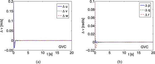
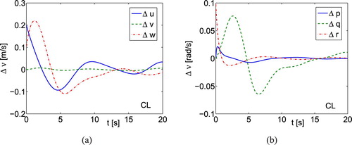
Figure 2. Simulation results using the classical (CL) controller for underwater vehicle: (a) linear velocity errors; (b) angular velocity errors.

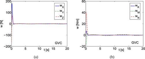
The applied forces and torques obtained from both control algorithms only differ slightly in both cases. Thus, they do not give you any important information about dynamic couplings. The lumped dynamics estimation errors $\text{w}$ related to linear and angular velocities (Figure 3(a,b)) tend to zero also very fast for the GVC controller what arises from that the whole system dynamics is included directly in the algorithm. They are not zero at the end because only convergence to a bounded neighbourhood ρ can be ensured (as it was shown in proof). In the first motion phase (Figure 8(a,b)) ${\text{w}}_X$, ${\text{w}}_Z$, ${\text{w}}_M$, and ${\text{w}}_N$ errors are great. It results from that we track velocities u, w, and r. Moreover, the disturbances ${\tilde{F}}_Z$ and ${\tilde{F}}_M$ have big values (${\tilde{F}}_N$ is smaller). This effect can also be explained by dynamic coupling. For the CL control algorithm, analogous values ${\text{w}}_X$, ${\text{w}}_Z$, and ${\text{w}}_M$ are not reduced so fast and they do not converge to small constant.

Figure 3. Simulation results using GVC for underwater vehicle: (a) lumped dynamics estimation errors $\text{w}$ related to linear velocities; (b) lumped dynamics estimation errors $\text{w}$ related to angular velocities.

Step 4. Using the proposed control algorithm, we are able to determine the kinetic energy related to each quasi-velocity ${\xi }_i$. In the case under study, the total kinetic energy is $K_E=519.47$ J. This energy is distributed as follows: $\delta K_{E1}=23.34$ %, $\delta K_{E2}=0.00$ %, $\delta K_{E3}=76.57$ %, $\delta K_{E4}=0.01$ %, $\delta K_{E5}=0.00$ %, $\delta K_{E6}=0.08$ %. It means that the most kinetic energy is reduced by ${\xi }_3$ (related mainly to w), and ${\xi }_1$ (related mainly to u). Really, the desired velocity is tracked in the directions z and x.

Step 5. At this stage, we evaluate the dynamical couplings using (33(33) $\mathrm{\Delta }{\xi }_i={\xi }_i-{\nu }_i,$(33) ) and (34(34) $\mathrm{\Delta }{\pi }_i={\pi }_i-{\tau }_i.$(34) ). It is possible only from the GVC controller. From Figure 4(a), it follows that the velocity v is deformed essentially ($\mathrm{\Delta }{\xi }_2$) but it is a small change (about 0.01 m/s). As shown in Figure 4(b), the deformation concerns the angular velocity p ($\mathrm{\Delta }{\xi }_4$). 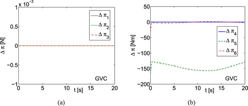Note that both these speeds are not tracked but should be zero. This fact can be explained by the presence of dynamic couplings in the vehicle. Considering Figure 5 we observe that only ${\tau }_M$ is deformed significantly ($\mathrm{\Delta }{\pi }_5$). It also results from couplings but additionally in this direction disturbances are also great.

Figure 4. Simulation results using GVC for underwater vehicle: (a) the quantity $\mathrm{\Delta }\xi$ time history related to linear velocities; (b) the quantity $\mathrm{\Delta }\xi$ related to angular velocities.

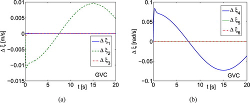
Figure 5. Simulation results using GVC for underwater vehicle: (a) the quantity $\mathrm{\Delta }\pi$ time history related to linear velocities; (b) the quantity $\mathrm{\Delta }\pi$ related to angular velocities.

Step 6 - Discussion of results-dynamics evaluation. If the proposed control algorithm is applied then an insight into the vehicle is available. Moreover, the velocity error convergence is simultaneous. Comparing the time history for the GVC and the CL algorithm we can determine which errors converge in long time ($\mathrm{\Delta }u$, $\mathrm{\Delta }w$, and $\mathrm{\Delta }q$). We can also identify that if even $q_d=0$ then $\mathrm{\Delta }q$ tends to zero very slowly (the control gain should be great in such a case). We have recognised that the applied forces and torques have similar values for the GVC and CL controller (for this reason they are omitted in the text). For the selected disturbances, the lumped dynamics estimation errors ${\text{w}}_X$, ${\text{w}}_Z$, and ${\text{w}}_M$ are big if the CL controller is used. This can be explained by the fact that that the appropriate disturbance forces and the moment have also great values. This effect makes it difficult to control the variable q because of internal coupling between this velocity and other velocities (compare $\mathrm{\Delta }q$ time history). As it can be expected the kinetic energy is reduced mainly by u and w (but here we can obtain quantitative answer). Some information about dynamical couplings (deformation of velocities v and p) we receive from the observation of $\mathrm{\Delta }{\xi }_i$ time history. From $\mathrm{\Delta }{\pi }_i$ we determined that the applied torque ${\tau }_M$ (related to q) changed essentially during the vehicle motion. We can say that q is strongly coupled with other velocities and it is sensitive for changes of other velocities and disturbances. Comparing the results from the GVC and CL algorithms it can be seen that in transformed dynamics case the results are better. The main reason for the differences is to use the same sets of control coefficients for both regulators. In the GVC controller, an additional gain results in the N matrix, thanks to which the control gains have higher values and are adequate to the dynamics of the vehicle. It is because we obtain the $k_D^{\ast }=N{k}_D$ and ${\mathrm{\Gamma }}^{\ast }=N\mathrm{\Gamma }$ instead of $k_D$ and Γ only. In the CL controller, this matrix is absent and the gain values do not provide an effective convergence of errors. However, such a comparison (between GVC and CL) makes sense if the primary goal of the study is to estimate the impact of dynamics on the behaviour of the vehicle because $k_D^{\ast }$ and ${\mathrm{\Gamma }}^{\ast }$ are dynamics dependent. Concluding, using the proposed control algorithm we are able to evaluate effect of couplings and dynamics at the stage of simulation studies.

Case 2: Comparative test of the controller.

In order to obtain a reasonable comparison of algorithms, a controller containing an adaptive term should be selected. The control approach which is based on such idea can be found in Soylu et al. (2008). However, that algorithm is implemented in the earth-fixed frame and is used to track the position trajectory. For this reason, it is therefore necessary to adapt this controller so that it is implemented in the body-fixed frame and enables velocity tracking instead of position tracking. After proper modification, the algorithm has the form (29(29) $\begin{array}{rl}\tau & =M{\dot{\nu }}_r+C\left(\nu \right){\nu }_r+D\left(\nu \right){\nu }_r+g\left(\eta \right)\\ & +k_{D}s+k_{I}z+\tilde{f},\end{array}$(29) ). For the test of the GVC algorithm, the set of gains (36(36) $k_D=12\cdot I,k_I=1\cdot I,$(36) ) is applied whereas for the controller (29(29) $\begin{array}{rl}\tau & =M{\dot{\nu }}_r+C\left(\nu \right){\nu }_r+D\left(\nu \right){\nu }_r+g\left(\eta \right)\\ & +k_{D}s+k_{I}z+\tilde{f},\end{array}$(29) ) only $k_I$ and Λ are the same (they do not include the dynamical parameters). To improve the error convergence, the values of $k_D$ and Γ matrices have been increased, i.e.: (40) $k_D=1000\cdot I,\mathrm{\Gamma }=6000\cdot I.$(40) These values are not related to the dynamics of the vehicle and they were chosen only to show the controller's performance (Figure 6). They must partially replace the lack of dynamic parameters of the vehicle in control gains. Comparing Figures 6(a,b) and 1(a,b) it can be seen that the GVC algorithm works faster (the end errors values are achieved faster than (29(29) $\begin{array}{rl}\tau & =M{\dot{\nu }}_r+C\left(\nu \right){\nu }_r+D\left(\nu \right){\nu }_r+g\left(\eta \right)\\ & +k_{D}s+k_{I}z+\tilde{f},\end{array}$(29) )). 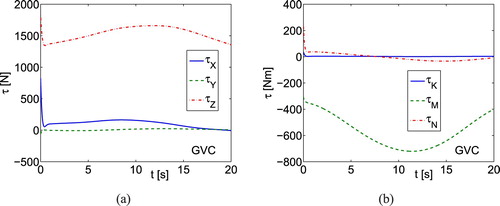Moreover, using (29(29) $\begin{array}{rl}\tau & =M{\dot{\nu }}_r+C\left(\nu \right){\nu }_r+D\left(\nu \right){\nu }_r+g\left(\eta \right)\\ & +k_{D}s+k_{I}z+\tilde{f},\end{array}$(29) ) more oscillations are observed but the controller works correctly. This is the effect of not taking into account the coupling and dynamics in the control gains. Similar observations and conclusions can be made by comparing Figures 6(c,d) and 3(a,b). From Figures 6(e,f) and 7(a,b), it is observed that the control forces and torques have comparable values for both controllers with exception of the first phase of motion. At the beginning, values of ${\tau }_X$ and ${\tau }_Z$ values are greater for the GVC algorithm than for the (29(29) $\begin{array}{rl}\tau & =M{\dot{\nu }}_r+C\left(\nu \right){\nu }_r+D\left(\nu \right){\nu }_r+g\left(\eta \right)\\ & +k_{D}s+k_{I}z+\tilde{f},\end{array}$(29) ). It can be said that the control effort is comparable for both controllers. The differences result from the use of dynamics in the GVC control scheme.

Figure 6. Case 2: simulation results using (29(29) $\begin{array}{rl}\tau & =M{\dot{\nu }}_r+C\left(\nu \right){\nu }_r+D\left(\nu \right){\nu }_r+g\left(\eta \right)\\ & +k_{D}s+k_{I}z+\tilde{f},\end{array}$(29) ) controller for underwater vehicle: (a) linear velocity errors; (b) angular velocity errors; (c) lumped dynamics estimation errors $\text{w}$ related to linear velocities; (d) lumped dynamics estimation errors $\text{w}$ related to angular velocities; (e) control forces τ; (f) control torques τ.

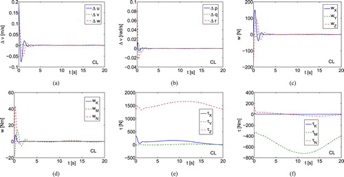
Figure 7. Case 2: simulation results using GVC for underwater vehicle: (a) control forces τ; (b) control torques τ.

As it results from Figure 6, we are able to ensure satisfactory performance of the controller (29(29) $\begin{array}{rl}\tau & =M{\dot{\nu }}_r+C\left(\nu \right){\nu }_r+D\left(\nu \right){\nu }_r+g\left(\eta \right)\\ & +k_{D}s+k_{I}z+\tilde{f},\end{array}$(29) ). However, based on these results it is impossible to estimate the dynamics of the vehicle by comparing the performance of this controller and the GVC algorithm (information concerning effects of dynamics is lost or inaccessible). The problem of improving the results obtained from the controller (29(29) $\begin{array}{rl}\tau & =M{\dot{\nu }}_r+C\left(\nu \right){\nu }_r+D\left(\nu \right){\nu }_r+g\left(\eta \right)\\ & +k_{D}s+k_{I}z+\tilde{f},\end{array}$(29) ) can be solved by individual selection of coefficients (for each matrix value $k_D$ and Γ) using the trial-and-error method which to some extent will replace the inclusion of the dynamic parameters.

6. Conclusions

In this work, a method for simulation analysis of underwater vehicle dynamic model based on the velocity tracking control algorithm in the presence of disturbances is proposed. It is realized after transformation of the velocity vector expressed in the body-fixed coordinates. After use of the controller, some advantages of the system dynamics are observable. Thus, the transformation allows one to give an insight into the dynamics of the vehicle. Applying the control algorithm, we can obtain fast system response and velocity error convergence. The procedure for dynamics evaluation is given and discussed, too. The considered here properties are not available in the same way without decomposition of the matrix of inertia. The proposed approach is applicable for fully actuated vehicles. The simulation analysis done on a 6-DOFs underwater vehicle illustrates the performance of the controller as well as the proposed dynamics evaluation method. The approach is useful both for control and for investigation of dynamic systems. This information can be served next for redesign of the construction. Therefore, the goal of the simulations is to deliver an information about the dynamical couplings and their role in the control of underwater vehicle. For further studies, the proposed method should be implemented in order to test it.

Disclosure statement

No potential conflict of interest was reported by the author.

ORCID

Przemyslaw Herman  http://orcid.org/0000-0002-8139-0236

Additional information

Funding

The work was supported by the Politechnika Poznańska University [grant number 09/93/DSPB/0611].

References

- ABS. 2006. ABS guide for vessel maneuverability. American bureau of shipping ABS plaza 16855 northchase drive houston. TX 77060 USA, March 2006 (Updated February 2017).
- Antonelli G. 2007. On the use of adaptive/integral actions for six-degrees-of-freedom control of autonomous underwater vehicles. IEEE J Oceanic Eng. 32(2):300–312. doi: 10.1109/JOE.2007.893685
- Barbalata C, De Carolis V, Dunnigan MW, Petillot Y, Lane D. 2015. An adaptive controller for autonomous underwater vehicles. Proceedings of the 2015 IEEE/RSJ international conference on intelligent robots and systems (IROS); Congress Center Hamburg; Sept 28–Oct 2, 2015. Hamburg, Germany. pp. 1658–1663.
- Bechlioulis CP, Karras GC, Heshmati-Alamdari S, Kyriakopoulos KJ. 2017. Trajectory tracking with prescribed performance for underactuated underwater vehicles under model uncertainties and external disturbances. IEEE Trans Control Syst Technol. 25(2):429–440. doi: 10.1109/TCST.2016.2555247
- Chen Y, Zhang R, Zhao X, Gao J. 2016. Tracking control of underwater vehicle subject to uncertainties using fuzzy inverse desired trajectory compensation technique. J Mar Sci Technol. 21:624–650. doi: 10.1007/s00773-016-0379-9
- Do KD, Pan J. 2009. Control of ships and underwater vehicles. London: Springer-Verlag London Limited.
- Donaire A, Romero JG, Perez T. 2017. Trajectory tracking passivity-based control for marine vehicles subject to disturbances. J Franklin Inst. 354:2167–2182. doi: 10.1016/j.jfranklin.2017.01.012
- Ferreira B, Matos A, Cruz N, Pinto M. 2010. Modeling and control of the MARES autonomous underwater vehicle. Mar Technol Soc J. 44(2):19–36. doi: 10.4031/MTSJ.44.2.5
- Fischer N, Hughes D, Walters P, Schwartz EM, Dixon WE. 2014. Nonlinear RISE-based control of an autonomous underwater vehicle. IEEE Trans Robot. 30(4):845–852. doi: 10.1109/TRO.2014.2305791
- Fossen TI (1994). Guidance and control of ocean vehicles. Chichester: Wiley.
- Garcia-Valdovinos LG, Salgado-Jimenez T, Bandala-Sanchez M, Nava-Balanzar L, Hernandez-Alvarado R, Cruz-Ledesma JA. 2014. Modelling, design and robust control of a remotely operated underwater vehicle. Int J Adv Rob Sys. 11(1):1–16. doi: 10.5772/56810
- Herman P. 2009. Decoupled PD set-point controller for underwater vehicles. Ocean Eng. 36:529–534. doi: 10.1016/j.oceaneng.2009.02.003
- Kim J, Joe H, Yu S-ch, Lee JS, Kim M. 2016. Time-delay controller design for position control of autonomous underwater vehicle under disturbances. IEEE Trans Ind Electron. 63(2):1052–1061. doi: 10.1109/TIE.2015.2477270
- Lee KW, Singh SN. 2016. Nonlinear adaptive trajectory control of multi-input multi-output submarines with input constraints. Proc IMechE Part I: J Sys Control Eng. 230(2):164–183.
- Liu S, Liu Y, Wang N. 2017. Nonlinear disturbance observer-based backstepping finite-time sliding mode tracking control of underwater vehicles with system uncertainties and external disturbances. Nonlinear Dyn. 88:465–476. doi: 10.1007/s11071-016-3253-8
- Soylu S, Buckham BJ, Podhorodeski RP. 2008. A chattering-free sliding-mode controller for underwater vehicles with fault-tolerant infinity-norm thrust allocation. Ocean Eng. 35:1647–1659. doi: 10.1016/j.oceaneng.2008.07.013
- Soylu S, Proctor AA, Podhorodeski RP, Bradley C, Buckham BJ. 2016. Precise trajectory control for an inspection class ROV. Ocean Eng. 111:508–523. doi: 10.1016/j.oceaneng.2015.08.061
- Spangelo I, Egeland O. 1994. Trajectory planning and collision avoidance for underwater vehicles using optimal control. IEEE J Oceanic Eng. 19(4):502–511. doi: 10.1109/48.338386
- Su Y, Zhao J, Cao J, Zhang G. 2013. Dynamics modeling and simulation of autonomous underwater vehicles with appendages. J Marine Sci Appl. 12:45–51. doi: 10.1007/s11804-013-1169-6
- Sun B, Zhu D, Ding F, Yang SX. 2013. A novel tracking control approach for unmanned underwater vehicles based on bio-inspired neurodynamics. J Marine Sci Technol. 18:63–74. doi: 10.1007/s00773-012-0188-8
- Vidyasagar M (1993). Nonlinear systems analysis. Englewood Cliffs (NJ): Prentice Hall.
- Yan Z, Yu H, Zhang W, Li B, Zhou J. 2015. Globally finite-time stable tracking control of underactuated UUVs. Ocean Eng. 107:132–146. doi: 10.1016/j.oceaneng.2015.07.039
- Yoon S-M, Hong S, Park S-J, Choi JS, Kim HW, Yeu T-K. 2012. Track velocity control of crawler type underwater mining robot through shallow-water test. J Mech Sci Technol. 26:3291–3298. doi: 10.1007/s12206-012-0810-2
- Zhu D, Sun B. 2013. The bio-inspired model based hybrid sliding-mode tracking control for unmanned underwater vehicles. Eng Appl Artif Intell. 26:2260–2269. doi: 10.1016/j.engappai.2013.08.017