Prediction of the density and viscosity of biodiesel and the influence of biodiesel properties on a diesel engine fuel supply system

Abstract

Biodiesel has been considering as promising fuel in the situation of ever-depleting fossil fuels and serious environment pollution. Beside clearly known advantages, high viscosity and density, and high surface tension are the acute disadvantages that need to be improved to use directly for an unmodified diesel engine. In this work, 24 samples of biodiesel–diesel fuel blends created by mixing respectively 5%, 10%, 20%, 40%, 50%, 60%, 75% and 100% of fractions of Coconut oil biodiesel (COB), Jatropha oil biodiesel (JOB), Waste oil biodiesel (WOB) in diesel fuel were used for experimental purposes. In the first stage, the effects of biodiesel fractions and temperature on kinematic viscosity and density were developed. In the second stage, the effects of kinematic viscosity and density on fuel supply system, fuel pump network, fuel filters, and spray characteristics (including penetration length (L_b) and Sauter Mean Diameter (SMD)) were investigated. Obtained results of this study based on experimental correlation and mathematical equation showed over 95% of the confident level from a regression correlation equation regarding kinematic viscosity and density.

1. Introduction

The ever-increasing demand for the energy and fuel has been one of the situations happening contrarily to the depletion of fossil fuel. Finding the renewable, environmentally friendly biofuels was considered as the extremely important task (Anh Tuan and Minh Tuan 2009; Rajagopal et al. 2016; Tran et al. 2017). Recently, besides other alternative fuels and several as-applied technologies for strategies of revewable energy (Hoang 2018b), biodiesel was widely used for transport sectors, as well as the scientific studies on biodiesel production, storage process, the influences of biodiesel usage on the performance of engines and emission characteristics have been increasing exponentially (Ioannou et al. 2013; Tuan et al. 2017). The explanation for using popularly biodiesel might be due to its advantages, being biodegradable, available, renewable, non-toxic, and carbon neutral (Work 2011; Ullah et al. 2014). Regarding the use of biodiesel for diesel engines, it could directly replace fossil diesel fuel without any major modifications (Hoang 2017). The reduction of incomplete oxidation products of combustion process such as unburned hydrocarbon (UHC) and carbon monoxide (CO), even a reduction of particulate matter (PM) was reported (Silitonga et al. 2017; Hoang and Pham 2018b). However, an insignificant increase in nitrogen oxides (NO_x) and CO₂ emission, exhaust gas temperature were also observed (Pushparaj et al. 2015).

Biodiesel was a product of the transesterification reactions of vegetable oil or animal fats with an alkanol, thus biodiesel was the ester of fatty acid with 17–19 total of carbon atoms. A strong alkaline catalyst or acid, and an enzyme were the main catalysts used in the transesterification reaction (Hoang and Le 2018). The difference in molecular structure resulted in significantly different physicochemical properties of biodiesel compared with those of fossil diesel fuel. Besides, this could also cause the effects on atomisation, evaporation, breakup, mixture formation, combustion processes, emission and pollutant formation (Hoang et al. 2018). Among properties of biodiesel, kinematic viscosity (KV), density (ρ) and heating value were seen as the main parameters, which mainly affected and played an important role in producing the engine power and forming emissions (Langfitt and Haselbach 2016; Hoang 2018a). High KV and ρ in comparison with fossil diesel fuel might lead to poor atomisation, long time of breakup and mixture formation, increase in carbon deposition on injectors and filters, more energy for pumping fuel, especially in small diesel engines (Satyanarayana and Muraleedharan 2011; An et al. 2012). The lean-burning phenomenon due to the slow movement of fuel through filter and lines caused by higher viscosity was indicated by some studies, the effect of viscosity on the injection start and pressure, the fuel spray characteristics were also reported (Raghavan et al. 2009; Lin et al. 2011). Meanwhile, crucial engine performance including power and specific fuel consumption was correlated against ρ because the variation of ρ affects the fuel mass supplied to engine (Zacharewicz and Kniaziewicz 2017). Some techniques such as blending the biodiesel with diesel or preheating biodiesel were used to improve the above disadvantages of biodiesel (Alptekin and Canakci 2008; Hoang and Van Le 2017). After blending or preheating, the KV and ρ of biodiesel were reduced, empirical correlations regarding the engine performance as well as emission data in the relationship with KV and ρ of biodiesel are reported (Bhale et al. 2009).

Regarding specific density (ρ) of biodiesel, it was defined as the ratio of fuel mass and fuel volume at the same condition about temperature and pressure. By using a standard- based-hydrometer method for experimentally measuring the density of pure soybean biodiesel (B100) and blends of fossil diesel fuel, being B20, B50 and B75 (20%, 50%, 75% of soybean biodiesel), Tat and Garpen (Tate et al. 2006) suggested 1st degree linear for the relationship between ρ and temperature. Also, the similar results were reported after being conducted for biodiesel of canola oil and fish-oil (Tat and Van Gerpen 2000), this relationship was indicated in Equation (A1). In another study, specific density of biodiesel was proposed as a function of the mass fractions of components contained in biodiesel (Yang et al. 2018). Hence, the specific density of biodiesel or its blends were also calculated as Equation (A2). Besides, the specific density of the biodiesel blend was also determined by the mass or volume percentage of components. The suggested equation by (Bhale et al. 2009) was an example where an experiment was carried out with six different biodiesels. After conducting this experiment, a 1st degree empirical equation in the correlation of the density of biodiesel–diesel fuel blends with the mass percentage of biodiesel was shown in Equation (A3), Equations from (A1) to (A3) are given in Appendix A.

Viscosity is a fluid property and it characterises the resistance to the flow of liquid. The viscous property was inversely proportional to the fluid velocity. Higher viscosity shows more unfavourable use, moreover, the sedimentation in the equipment, poor atomisation, and difficult evaporation are the consequences of high viscosity or maintaining incorrect temperature (Hoang and Pham 2018a). Normally, biodiesel viscosity was insignificantly higher than that of conventional diesel fuel at 40°C. However, at a lower temperature, biodiesel viscosity tended much higher, especially below 25°C. There were some methods to reduce biodiesel viscosity, being preheating, blending or using additives (Hoang and Nguyen 2017). Based on the laws of Grun-Nissan and Katti-Chaudhri, biodiesel viscosity was estimated in a mathematical formula that was shown in Equation (B1) (Riazi and Al-Otaibi 2001). Similar to Equation (A2), biodiesel viscosity was also a function of mass percentages of biodiesel in the blends. However, the 2nd degree empirical equation might be more suitable for the relationship between biodiesel viscosity and mass percentage, this empirical equation was estimated through Equation (B2). Another method for estimating and predicting the fluid viscosity originated from hydrocarbons or petroleum mixtures shown in Equation (B3) was also proposed by Joshi and Pegg (Joshi and Pegg 2007), although this equation was not used popular due to the difficulty in the determination of input molecular weight as well as and the refractive index of compounds. By considering the viscosity of biodiesel as a function of temperature, the Equation (B4) was developed to calculate the dynamic viscosity of pure biodiesel in the range of temperature from 5°C to 300°C with 22.3% of absolute error and correlation coefficient R² of 1 (Fasina and Colley 2008), the exponential model was also suggested as Equation (B5) (Krisnangkura et al. 2006). The carbon chain structure was also proposed in the correlation with biodiesel viscosity (Yamane et al. 2001). Equations (B6) and (B7) were considered to determine biodiesel viscosity based on carbon number at different temperatures. Equations from (B1) to (B7) are given in Appendix B.

The dependence of empirical correlations, being specific density and kinematic viscosity of biodiesel types, on constants, mass or volume percentage of components in blends could be seen clearly from above-described equations. Moreover, as reported, specific density and kinematic viscosity were two main parameters, which were of immense using in the engine field, the simulation, and modelling of combustion, exhaust emission (Ushakov et al. 2013). Furthermore, the dynamic phenomena of the fluid flow in the fuel pump, fuel pipe, and filter, as well as spray characteristics and breakup regime were strongly affected by biodiesel properties. Thus, the establishment of a simple, stable and highly confident estimation method for KV and ρ in the relationship with biodiesel fraction and temperature was very important. The aim of this work was to determine a correlation between biodiesel KV, ρ, and temperature, fraction. Moreover, the influence of biodiesel KV and ρ on the fuel supply system was also investigated and quantified.

2. Materials and methods

2.1. Materials

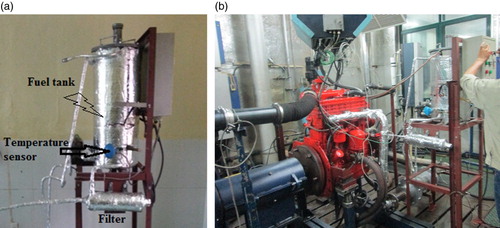
In this study work, three types of biodiesel such as Coconut oil biodiesel (COB), Jatropha oil biodiesel (JOB) and Waste oil biodiesel (WOB) available in Vietnam were used for analysis purpose. COB and JOB were the commercial biodiesel types, WOB was only produced with the pilot scale. All three biodiesel types were also produced by transesterification-based-reactions with methanol and additives, meanwhile, fossil diesel fuel was supplied by The Vietnam National Petroleum Group (Petrolimex). Table 1 gave the properties of three types of pure biodiesels and fossil diesel fuel (DF).

Table 1. Properties of COB, JOB, WOB, and DF at 30°.

Properties	Abbreviation	Unit	Standards	Requirement	COB	JOB	WOB	DF
Density	ρ	kg/m^3	ASTM D1298	860–900	878	880	883	852
Kinematic viscosity	KV	cSt	ASTM D 445	min 1.9	6.2	6.5	6.8	3.5
Cetane number	CN		ASTM D 613	min 47	70	50	52	45
Flash point	TF	°C	ASTM D 93	min 130	110	166	180	55
Calorific value	HV	MJ/kg	ASTM D2015-85	min 40	40.5	41	39.5	43

A 5%, 10%, 20%, 40%, 50%, 60%, 75% and 100% of volume percentage of COB, JOB, WOB were blended with DF at the same surrounding ambient condition to determine the effect of fraction biodiesel on KV and ρ. However, 100% biodiesel of samples were used for determining the effect of temperature on KV and ρ of biodiesels. Totally, there were 25 biodiesel samples (including a sample of diesel fuel) used to measure the KV and ρ, the influence of KV and ρ on the fuel supply system was investigated and calculated based on as-obtained results.

2.2. Methods

2.2.1. Viscosity and density measurement

For measuring density in a relationship with temperature and fraction, the ASTM D1298 standard procedure was used. A glass hydrometer for measuring density in the range of 0.7–1.0 g/cm³ with three decimal number of accuracy was considered. To collect temperature-depending data, a cylinder with 100 ml of the volume containing the sample was placed in a bath with controlled temperature from 30°C to 100°C. The test was repeated three times to take the average value.

The ASTM D 445 standard was used to measure the effect of temperature and fraction of the samples on kinematic viscosity. The kinematic viscosity was determined based on measuring the time of a known volume of sample flowing under gravity to pass through a calibrated glass capillary viscometer tube at the room conditions. CANNON Viscometer tube was used for this purpose with viscometer constants of 0.0359 and a viscosity range of 2–30 cSt. In case of determining the effect of kinematic viscosity on temperature, the used water bath had a range from 30°C to 100°C of temperature. For the experimental data to be acceptable, the ASTM D 445 standards required the tests to be done two times with an accuracy of 0.02 cSt. The average value was considered as a representative value with satisfactory precision.

2.2.2. Measurement of the effect of fuel properties on fuel supply system

The friction head loss and flow rate are two important parameters used to evaluate the effect of viscous force to the motion ability of liquid fuel currency from the fuel pump to fuel filter through the fuel pipe. Meanwhile, Sauter mean diameter (SMD), length and cone angle of fuel spray show the quantity of fuel injection. However, it was difficult to determine the effects versus experimental study, thus a well-accepted mathematical model might be more suitable for predicting above affected parameters under the different operating conditions of the engine. The characteristics of the D243 diesel engine used for the prediction model were briefly described in Table 2.

Table 2. Technical parameters of diesel engine D243.

Technical parameters	Unit	Quantity
Type		Vertical4-strokeDirect injectionCooled by water
Model		D243 from Belarus
Number of cylinders	i	4
Rated power	HP	80
Maximum revolution	rpm	2200
Bore	mm	110
Stroke	mm	125
Displacement	litter	4.75
Compression ratio	ϵ	16.7:1
Nozzle hole diameter	mm	0.25

In the fuel supply system, the filter is an important component. The primary application of filter is to ensure extraneous matters and impurities of which the sizes are bigger than the requirement, as well as the fraction of water, removed from the fuel before supplying to the engine. Volume flow rate of fuel was used to estimate the effect of fuel properties on the filter, and volume flow rate was known as a more suitable parameter than mass flow rate because of its independence to density. To determine the volume flow rate of fuel, the using fuel system of the engine for producing the power corresponding to the flow rate of fuel was presented in Figure 1. Fuel flow rate (FR) was determined by a volume flow metre that was mounted at the outlet of the filter in a determined duration. The characteristics of fuel flow through the filter were described by Equations (1) and (2) in case of constant pressure (Lefebvre and McDonell 2017). Equation (2) showed that the FR was inversely proportional to KV of fuel in the filter and it showed the simple determination of FR. Therefore, this study used Equation (2) for presenting the relationship between the fuel flow rate (FR) and time (t) with a variation of KV. (1) $\frac{V^2}{2}=\frac{S^2\left(\mathrm{\Delta }P\right)t}{\lambda .\text{KV}.v}$(1) (2) $\text{FR}=\frac{C}{\text{KV}.t}$(2) Where: V - the volume of fuel passing through the filter, m³; t - time, s; S - a cross-sectional area of the filter cake, m²; ΔP - applied pressure difference, Pa; λ - constant depending on filtration resistance; v - the volume of cake deposited by unit volume of fuel; C - constant depending on filtration property

Figure 1. A fuel supply system-mounted- filter coupling to D243 diesel engine.

High KV tends to prevent the motion of fuel flow and it affects strongly the pump working-characteristic. This effect is evaluated through the head loss appearing in the pump network. As reported, the head loss occurring in fuel pipes depended on some parameters, being flow velocity, pipe dimension, friction factor, and Reynolds number (Re). The frictional head loss (H_f) value might be calculated by the following equation: (3) $H_f=\mathrm{2.4384.}{F}_f.L_e.\frac{u^2}{2g}$(3) Where:

• H_f - friction head loss, m

• F_f - dimension-less friction factor, (4) $F_f=\frac{0.0396}{{\mathrm{Re}}^{0.25}}$(4)

• $L_e=L/d$- the equivalent ratio of pipe length (L) to pipe diameter (d)

• u - initial velocity of fuel, m/s. The velocity of fuel can be calculated as an equation that was suggested in reference (Hiroyasu et al. 1989). $u=\sqrt{\frac{2\mathrm{\Delta }P}{{\rho }_l}}$

• ΔP - differential pressure between injection pressure and pressure in the cylinder during the injection period, bar

• g - gravitational acceleration, m/s².

The quality of fuel–air mixture in the combustion chamber is much affected by the atomisation process, which is characterized by three parameters of penetration length (L_b), spray angle (θ) and Sauter mean diameter (SMD). However, SMD and L_b are considered as the main factor affecting directly the evaporation of fuel droplet, SMD is calculated as the ratio of droplet volumes sum to surface areas sum, the higher the surface areas sum is, the lower the SMD is. Some models were purposed to correlate SMD and fuel properties, Hiroyasu and Arai model was an example (Krisnangkura et al. 2006): (5) $\frac{\text{SMD}}{D}=\mathrm{0.38.}{\mathrm{Re}}_l^{0.25}{\text{We}}_l^{-0.32}(\frac{{\mu }_l}{{\mu }_g}{)}^{0.37}{\left(\frac{{\rho }_l}{{\rho }_g}\right)}^{-0.47}$(5) (6) $L_b=7.D.\left(1+0.4\frac{r}{D}\right).{\left(\frac{p_g}{{\rho }_l{u}^2}\right)}^{0.05}.{\left(\frac{L}{D}\right)}^{0.13}.{\left(\frac{{\rho }_l}{{\rho }_g}\right)}^{0.5}$(6) Where: $\text{W}{\text{e}}_l=\frac{u^{2}D}{{\sigma }_l}{\rho }_l$ - Weber number; $\text{R}{\text{e}}_l=\frac{uD}{{\mu }_l}{\rho }_l$- Reynolds number; ρ_l - the density of the fuel, kg/m³; ρ_g - the density of the gas, kg/m³; μ_l - fuel dynamic viscosity, N.s/m²; μ_g - gas dynamic viscosity, N.s/m²; D - nozzle hole diameter, mm; σ_l - fuel surface tension, N/m.

3. Results

3.1. The relationship between biodiesel density and fraction, temperature

This section may be divided by subheadings. It should provide a concise and precise description of the experimental results, their interpretation as well as the experimental conclusions that can be drawn. As injected into the combustion chamber, the chain ‘atomization → breakup → mixture’ is affected strongly by fuel density and viscosity, and that is an accepted fact. Hence, the knowledge of the temperature and fraction dependence of fuel density is a key component to optimise the combustion process. From Equations (A1)–(A3) show that biodiesel density is a function of temperature and fraction. Density values of blends of three biodiesel types are given in Table 3 where ρ₁, ρ₂, ρ₃ are density values that are calculated by the ratio of mass and volume, by Equation (A2), and measured by a hydrometer, respectively. Meanwhile, Δ₁ and Δ₂ are considered as the absolute percentage error of ρ₁ compared with ρ₃, ρ₂ compared with ρ₃ respectively. Figures 2–4 show the increase in density of biodiesel-fossil diesel blends, this increase is inversely proportional to the increase of biodiesel fractions.

Figure 2. The dependence of density on COB fraction.

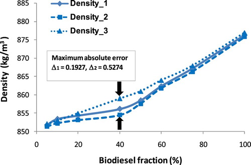
Figure 3. The dependence of density on JOB fraction.

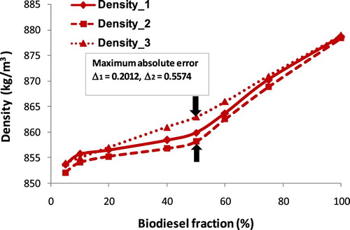
Figure 4. The dependence of density on WOB fraction.

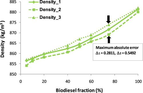
Table 3. Measurement and calculation methods for biodiesel blend density at 30°C.

Biodiesel types	Biodiesel fraction (%)	ρ1 , kg/m^3	ρ2, kg/m^3	ρ3, kg/m^3	Δ1	Δ2
COB	5	851.75	851.36	852.00	0.0470	0.0751
	10	853.41	852.22	853.00	0.1394	0.0914
	20	854.38	853.14	855.00	0.1451	0.2175
	40	856.12	854.47	859.00	0.1927	0.5274
	50	858.48	857.54	861.00	0.1095	0.4019
	60	862.34	861.78	864.00	0.0649	0.2569
	75	867.25	866.35	868.00	0.1038	0.1901
	100	876.30	875.87	877.00	0.0491	0.1288
JOB	5	853.66	852.12	854.00	0.1804	0.2201
	10	855.71	854.08	855.00	0.1905	0.1076
	20	856.58	855.23	857.00	0.1576	0.2065
	40	858.47	856.85	861.00	0.1887	0.4820
	50	859.92	858.19	863.00	0.2012	0.5574
	60	863.73	862.55	866.00	0.1366	0.3984
	75	870.28	868.87	871.00	0.1620	0.2445
	100	878.77	878.44	879.00	0.0376	0.0637
WOB	5	856.53	854.18	857.00	0.2744	0.3291
	10	857.46	856.32	858.00	0.1330	0.1958
	20	859.68	858.21	860.00	0.1710	0.2081
	40	862.45	860.66	864.00	0.2075	0.3866
	50	864.51	863.27	867.00	0.1434	0.4302
	60	867.32	865.81	869.00	0.1741	0.3671
	75	871.65	869.2	874.00	0.2811	0.5492
	100	881.49	880.08	882.00	0.1600	0.2177

Obviously, Figures 2–4 show that the maximum absolute error tends to change along with the variation of biodiesel faction. This absolute error for COB gets the maximum at 40% of the fraction, for JOB gets the maximum at 50% of a fraction, and for WOB gets the maximum at 75% of the fraction. This alteration can be explained due to ρ(WOB) > ρ(JOB) > ρ(COB), the increase of the fraction of biodiesel with a higher density results in the value of the absolute error between the calculation and experiment getting the maximum at the point with a higher fraction. However, absolute error (Δ₃) and (Δ₄) get the maximum at the same point.

From Table 3, it can be seen that the density values of biodiesel blends increase along with the increase in volume fraction of each biodiesel types. The maximum absolute error of Δ₁ and Δ₂ is 0.2811% and 0.5574%, respectively. Also, the density values of 24 samples at each point corresponding to the same volume fraction are very close, resulting in a 1st degree regression equation for the relationship between density and fraction biodiesel. This correlation equation is presented in Figure 5 and Equation (17) when x is considered as biodiesel fraction. (7) ${\rho }_{\mathrm{b}\mathrm{i}\mathrm{o}\mathrm{d}\mathrm{i}\mathrm{e}\mathrm{s}\mathrm{e}\mathrm{l}}=0.2558x+852.08$(7)

Figure 5. The relationship between density and fraction of three studied biodiesel types (a), the regression correlation of experimental values (b).

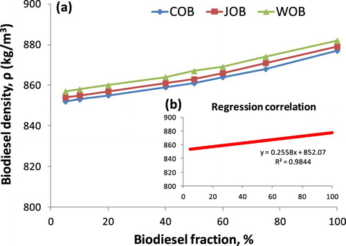
Table 3 and Figure 5 show that the regression correlation of experimental values has R² of 0.9844. This proves that as diesel and biodiesel density are known clearly, Equations (A2) and (7) are used the confident methods to predict and determine biodiesel density with the variation of biodiesel fraction in biodiesel–diesel blends. The maximum absolute error of biodiesel density as using Equation (7) in comparison with hydrometer-based-measured values is 0.4956% for WOB, 0.2012% for JOB and 0.4463% for COB. In another experiment, biodiesel density considered as a function of temperature is established that the densities of three pure biodiesel types are measured in the range of temperature of 30–100°C. Results from Table 2 show that the biodiesel density is higher than that of studied DF. However, heating biodiesel at a temperature of 80°C or higher is a suitable temperature to ensure that biodiesel density is equal to or below 850 kg/cm³, corresponding to European standard (CEN. EN 14214:2008 2010; Tat and Van Gerpen 2000). The influence of temperature (T) on density is shown in Figure 6 and Equation (8). (8) ${\rho }_{\mathrm{b}\mathrm{i}\mathrm{o}\mathrm{d}\mathrm{i}\mathrm{e}\mathrm{s}\mathrm{e}\mathrm{l}}=-0.5T+894.58$(8)

Figure 6. The relationship between density of three types of pure studied biodiesels and temperature (a), the regression correlation of experimental values (b).

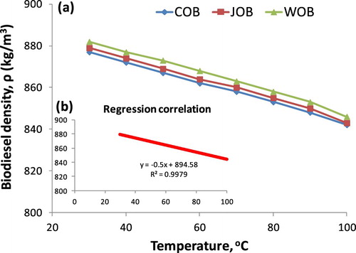
The regression correlation of experimental values regarding biodiesel density and temperature can be observed clearly in Figure 6 and Equation (8) where the inverse proportion between density and temperature is indicated with R² = 0.9979. This result is the same as the reported studies (Tesfa et al. 2010; Esteban et al. 2012). Compared with experimental measurement, the maximum absolute error by using Equation (8) is 0.3055% for COB, 0.1871% for JOB and 0.4026% for WOB. The small error as using Equation (7) and (8) and empirically measured values may be due to a small difference in the density of three biodiesel samples. In fact, the density of three biodiesel samples ranges from 878 kg/m³ to 883 kg/m³. The analysis results indicate that the heating method is considered the simplest one to reduce the density of biodiesel without changing cetane number as well as heating value. However, a blend of biodiesel-DF only operates with decreasing the density compared with pure biodiesel but the density values of biodiesel-DF blends are always higher than that of DF. In fact, these two methods, being blend and heating method, may be applied to diesel engines. In some engine types and configurations, being combined heat and power (CHP), biodiesel or biodiesel-DF blend may be used at lower injected-temperatures (Marengo et al. 2009). Table 3, Figures 5 and 6 present the most relevant parameters regarding the relationship of density-fraction and density-temperature, as shown in Equations (7) and (8). Once the statistical model means are used to determine and adjust the regression correlation of experimental data, a fit criterion is necessary to establish (Montgomery et al. 2006). Using the F-test approach, the statistical model is only significant with a confidence level of 95% (Tat and Van Gerpen 2000). Results from in Figures 5 and 6 indicate that the relationships of density-temperature and density-fraction can be considered by means of a straight line with a high confidence level, respectively 99.79% and 98.44%. The above small error values imply that Equations (7) and (8) can be used to predict and estimate fraction-based-density and temperature-based-density of the biodiesel blend.

3.2. The relationship between biodiesel kinematic viscosity and fraction, temperature

The estimation of KV of biodiesel blend is to aim at determining the suitable ratio of mixing based on meeting the requirement of good atomisation and fast evaporation as well as forming the homogeneous mixture. KV of biodiesel blends depending on the fraction is shown in Figure 7.

Figure 7. The relationship between KV and studied biodiesel fraction.

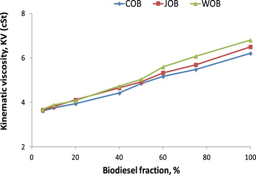
It is seen clearly a proportional relationship between KV and biodiesel fraction from Figure 7 that the increase in biodiesel fraction results in increasing KV. Based on the empirical results, a second-degree equation as Equation (9) is suggested. The A, B and C empirical coefficients, value R², calculated kinematic viscosity by Equation (B1) (KV₁), measured kinematic viscosity (KV₂) and calculated kinematic viscosity by Equation (9) (KV₃) are given in Table 4. Besides, the absolute error of KV between empirical Equation (9) and measured parameters (Δ₃), between empirical Equation (9) and calculated results by Equation (B1) (Δ₄) are also reported in Table 4. Figures 8–10 show the increase in kinematic viscosity of biodiesel-fossil diesel blends depending on biodiesel fractions. (9) $\text{KV}=A{x}^2+Bx+C$(9) The provided variation trends (from Figures 8–10) of KV of biodiesel-fossil diesel fuel blends seem to be different from those of ρ of biodiesel-fossil diesel fuel blends. The reason, which is used to explain, is due to the correlation between KV and biodiesel fraction is a logarithmic function or 2nd degree regression equation; meanwhile, the correlation between ρ and biodiesel fraction is a 1st degree regression equation. This trend leads to the absolute error (Δ₃) and (Δ₄), which do not get the maximum at the same point.

Figure 8. The dependence of kinematic viscosity on COB fraction.

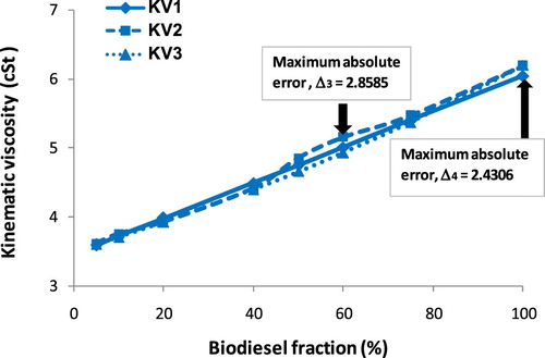
Figure 9. The dependence of kinematic viscosity on JOB fraction.

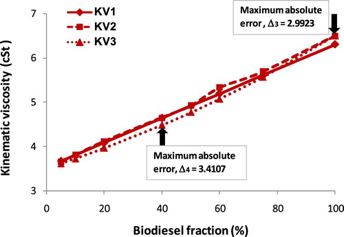
Figure 10. The dependence of kinematic viscosity on WOB fraction.

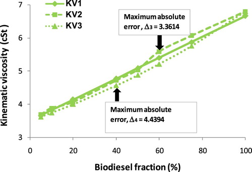
Table 4. KV values of biodiesel blends at 30°C.

Biodiesel types	Biodiesel fraction (%)	A	B	C	R^2	KV1, cSt	KV2, cSt	KV3, cSt	Δ3, %	Δ4, %
COB	5	2.10^−5	0.0259	3.4573	0.9952	3.5869	3.61	3.6015	0.6399	0.4056
	10					3.7165	3.75	3.7060	0.8933	0.2845
	20					3.9757	3.93	3.9240	1.1628	1.3167
	40					4.4941	4.41	4.3994	1.9070	2.1516
	50					4.7533	4.85	4.6583	1.9938	2.0388
	60					5.0125	5.16	4.9324	2.8585	1.6230
	75					5.4013	5.47	5.3742	1.2559	0.5050
	100					6.0493	6.20	6.2000	2.4306	2.4306
JOB	5	2.10^−5	0.0278	3.5235	0.9988	3.6626	3.65	3.6100	0.3452	1.4563
	10					3.8017	3.81	3.7235	0.2178	2.0999
	20					4.0799	4.11	3.9613	0.7324	2.9941
	40					4.6363	4.65	4.4834	0.2946	3.4107
	50					4.9145	4.92	4.7697	0.1118	3.0359
	60					5.1927	5.33	5.0743	2.5760	2.3335
	75					5.61	5.69	5.5680	1.4060	0.7537
	100					6.3055	6.50	6.5000	2.9923	2.9923
WOB	5	2.10^−5	0.0317	3.4989	0.9943	3.6575	3.68	3.6182	0.6114	1.0868
	10					3.8161	3.88	3.7403	1.6469	2.0252
	20					4.1333	4.07	3.9972	1.5553	3.4048
	40					4.7677	4.72	4.5650	1.0106	4.4394
	50					5.0849	5.04	4.8785	0.8909	4.2303
	60					5.4021	5.59	5.2135	3.3614	3.6168
	75					5.8779	6.07	5.7597	3.1647	2.0525
	100					6.6709	6.80	6.8000	1.8985	1.8985

It can be concluded from Table 4 and Figure 7 that, obtained KVs of the biodiesel blends as the biodiesel fraction in the range of 5% to 100% are 3.61 cSt to 6.80 cSt from the experiment, 3.5869 cSt to 6.6709 cSt from Equation (9), 3.6015 cSt to 6.80 cSt from Equation (B1). The maximum absolute error is 4.44% in comparison of Equation (9) with Equation (B1), and this maximum value is 3.36% in comparison of Equation (9) with the empirical equation. However, this maximum absolute error is lower than 5%, thus the correlation by a second-degree equation with R²≈ 1 is acceptable with high reliability. With reasonable accuracy, both Equations (9) and (4) can be used to estimate the KV of biodiesel blends if pure biodiesel KV and diesel fuel are known clearly. In another case, the effect of temperature on biodiesel KV with a temperature range of 30°C to 80°C is plotted in Figure 11.

Figure 11. The relationship between KV and temperature of three studied biodiesel types.

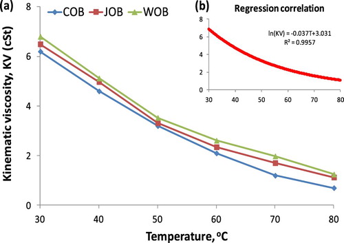
The empirical correlation for KV and heating temperature is observed in Figure 11. It can be described as a logarithmic function, being Equation (10), with an R² value of 0.9957. The obtained Equation (10) is similar to the past studies (Riazi and Al-Otaibi 2001; Joshi and Pegg 2007). (10) $\ln \left(\text{KV}\right)=-0.037T+3.031$(10) Similar to section 3.1, the limited confidence level of 95% can be seen from Table 4 and Figure 11. Thus, a second-degree equation is used for estimation of fraction-based-KV function, the logarithmic function is considered more suitable for temperature-based-KV correlation. Besides, a mathematical expression or equation for linking two key parameters of biodiesel such as density and KV is very valuable. Based on this approach, the determination of biodiesel KV is simple and fast if known biodiesel density. The biodiesel KV-density relationship depending on biodiesel fraction is presented in Figure 12, and biodiesel KV-density relationship depending on temperature is plotted in Figure 13.

Figure 12. KV and density of three studied biodiesel types with fraction variation.

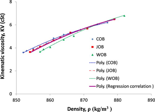
Figure 13. KV and density of three studied biodiesel types with temperature variation.

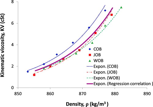
To characterise the diesel–biodiesel blend KV as a function of their density values with fraction and temperature variation, a regression correlation is carried out and is shown in Figures 12 and 13, leading to a correlation equation given in Equations (11) and (12). Results presented in Figures 12 and 13 are quite favourable with respectively R² = 0.9961 and R² = 0.9978 of confidence level. (11) $\text{KV}=-0.017{\rho }^2+3.0034\rho -1346.2$(11) (12) $\text{KV}={\mathrm{3.68.10}}^{-28}\exp \left(0.074\rho \right)$(12)

Results indicated in Equations (11) and (12) show a good estimation of the diesel–biodiesel blend KV by the measured density of diesel–biodiesel blend in both cases of biodiesel fraction variation and temperature variation. The above correlations are similar to past studies such as (Tat and Van Gerpen 1999; Tesfa et al. 2010; Tesfa et al. 2010).

3.3. Effect of biodiesel density and biodiesel viscosity on the fuel system

The fuel supply system of the diesel engine is to provide the necessary fuel according to the working mode of the engine, to provide a uniform fuel for the right engine cylinder and in the correct time, to atomize and disperse the fuel evaporation into the combustion chamber. In addition, the fuel supply system must ensure for the engine working continuously during the designed time or distance and separate the water and mechanical impurities without hindering the flow of fuel in the system. The above-mentioned requirements of fuel supply system request the fuel properties to meet the standards. While the values of KV and density of biodiesel are higher than the required ones based on ASTM standard, or the fuel is supplied to engines with incorrect and unsuitable KV compared to engine maker recommendations, they will affect negatively the components in the fuel supply system such as a pump, filter, and result in poor atomisation and spray as well as incomplete combustion. The relationship between FR through filter and time with different values of kinematic viscosity is shown in Figure 14. Besides, H_f calculated by from Equation (5) with the differential empirical pressure ΔP of 160 bar, the ratio L/d = 2000mm/25 mm is given in Table 5.

Figure 14. The relationship of FR through filter and time at different values of kinematic viscosity.

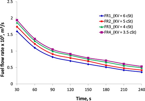
Table 5. H_f characteristics of the fuel pump at different values of kinematic viscosity.

KV, mm^2/s	u, m/s	Ff	Hf, m
6	191.7853	0.007448	2.672021
5	192.4501	0.007110	2.568469
4	193.1218	0.006718	2.443965
3.5	193.8006	0.006492	2.378284

Figure 14 shows that FR is inversely proportional to KV of fuel. These results are due to the ratio of active voidage and the total volume of filtration is high during the starting period. This ratio is certainly decreased after a while of working, resulting in a constant filtration rate, which is clearly seen in Figure 14, especially after about 180s. On the average result, the FR through the filter at KV fuel of 3.5 cSt is 33.40%, 18.34%, and 5.99% higher than that of KV fuel of 6 cSt, KV fuel of 5 cSt, and KV fuel of 4 cSt, respectively. Besides, H_f value at low KV is also smaller than that at high KV, the H_f value at KV fuel of 3.5 cSt is 10.99%, 7.40%, and 2.69% lower than that of KV fuel of 6 cSt, KV fuel of 5 cSt, and KV fuel of 4 cSt, respectively. Thus, this can prove that the fluid with higher KV leads to higher flow resistance, and it is the main cause of the increase in H_f and decrease of FR of liquid fuel as flowing through the filter. The same results are also reported by another study (Bannikov et al. 2006; Baumgarten 2006).

3.4. Effect of biodiesel density and biodiesel viscosity on spray characteristics

The quality of the air–fuel mixture in the engine cylinder depends on the size, homogeneity of the fuel droplets after being injected. The smaller the fuel droplet size is, the greater the heated and evaporated total area is, the faster the evaporation rate is. Spraying homogeneously is the key factor in creating a homogeneous mixture (Hoang and Pham 2018a). The uniformity and homogeneity of the fuel spray and atomisation are evaluated through the diameter of the fuel droplets and particles. Besides, the dispersion of fuel droplets and particles is characterized by the mean diameter of the particles as injected. Fuel particle size gives an overview of the level of fuel dispersion.

Multiple indicators characterise the fuel injection quality, but the most important indicator is smoothness, uniformity, length and cone angle of the fuel spray. The quality of the fuel injection into the engine combustion chamber depends on the injection pressure, the size of the injection nozzle, the quality of the high-pressure pump, the viscosity and density of the fuel. Figures 15 and 16 show the correlation of SMD and L_b with fuel KV under considering the different speed of the engine.

Figure 15. SMD as a function of KV at a different revolution of the test engine.

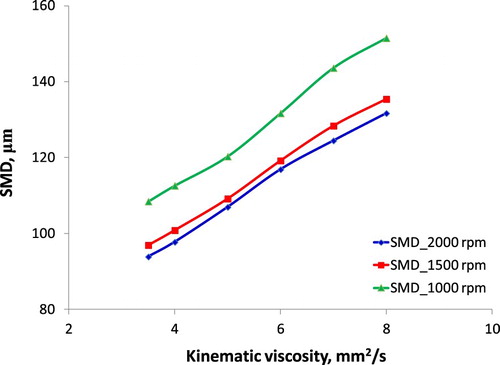
Figure 16. Penetration length as a function of KV at a different revolution of the test engine.

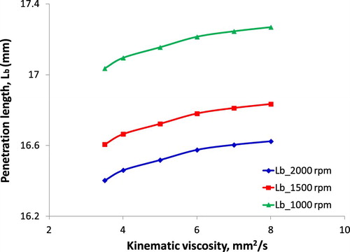
Based on Hiroyasu and Arai as-described model in Equation (6), it can be seen an increase of fuel SMD which is injected into the combustion chamber when the engine speed is changed. Obviously, besides of KV, the engine speed significantly affects SMD and L_b. At low speed, fuel injection velocity and injection pressure are the main cause leading to larger SMD and longer L_b at the same KV value. However, at the same engine speed, the increase in fuel KV resulting in an increase in surface tension has been proved (Aminul Islam et al. 2015). Moreover, high KV and high surface tension are due to high molecular mass and long-chain structure and cause the difficulty of fuel evaporation and breakup. Both primary breakup and secondary breakup depend on fuel properties, meanwhile, the fuel spray characteristics depend on the primary breakup and the time of breakup and mixture formation depend on the secondary breakup. Along with short time since injection starts to combustion start, smaller SMD and shorter L_b are the accordant parameters for good combustion. Results about the effect of fuel KV on the combustion process, resulting in affecting the engine performance and emission characteristics have indicated by (An et al. 2012; Hoang and Nguyen 2017). The obtained results in this study are similar to the past study (Gao et al. 2009).

4. Conclusion

Based on the changes of ambient temperature and fraction of biodiesel, the dual model for estimation of kinematic viscosity and density of biodiesel–diesel fuel blends based on three biodiesel types such as Coconut oil biodiesel (COB), Jatropha oil biodiesel (JOB), and Waste oil biodiesel (WOB) is developed. Some following results are reported as followed:

1. An inverse proportion between kinematic viscosity and density of biodiesel–diesel fuel blends and temperature is shown; meanwhile, the increase of kinematic viscosity and density of biodiesel–diesel fuel blends in a proportion to biodiesel fraction is also demonstrated. This means that heating method or blending method is considered as the simple one to decrease the kinematic viscosity and density of biodiesel according to the fuel requirements for diesel engines or the engine maker recommendations. In fact, blends of biodiesel–diesel fuel with the above-mentioned properties meeting well requirements and recommendations provide a good atomisation, fast evaporation and a formation of the homogeneous mixture which aid the diesel engines to achieve the best combustion aiming to produce the maximum of power and the minimum of pollution emission.

2. Empirical equations to estimate the properties of biodiesel–diesel fuel blends with high confidence level are developed.. In the relationship between the density of biodiesel–diesel fuel blends and temperature, R² reaches a high value at 0.9979. For the prediction of the density according to volume fractions, the value R² at 0.9844 is shown. Regarding the prediction of kinematic viscosity, the high value R² at 0.9942 for the correlation of kinematic viscosity and temperature, and 0.9957 for the correlation of kinematic viscosity and volume fractions are concluded. Besides, based on the experimental data and model, a function for the correlation of kinematic viscosity and density are also presented with 0.9961 of R² value.

3. Fuel flow rate and frictional head loss are evaluated based on the mathematical equation. High density and kinematic viscosity are considered the main causes resulting in low fuel flow rate and high frictional head loss at the same duration of carrying out the experiment.

4. The dependence of SMD and penetration length on kinematic viscosity when test engine is operated at various speeds is also presented as a proportion relationship, which is used to explain the reason of poor atomisation and evaporation, incomplete combustion as using fuel with high kinematic viscosity.

5. In general, this study provides the method to determine the ratio mixing for biodiesel and diesel fuel based on experimental data and empirical equations. The choice of suitable ratio mixing of biodiesel and diesel fuel depends on the requirements related to kinematic viscosity. In the following study, the use of biodiesel–diesel fuel blends for diesel engines will be conducted to get the experimental results such as engine performance, emission characteristics aiming at evaluating sufficiently the applicability of biodiesel and the effects of biodiesel on the fuel supply system.

Disclosure statement

No potential conflict of interest was reported by the author.

Appendices

Appendix A. Equation for density prediction

(A1) ${\rho }_{\mathrm{b}\mathrm{i}\mathrm{o}\mathrm{d}\mathrm{i}\mathrm{e}\mathrm{s}\mathrm{e}\mathrm{l}}=a+bT$(A1) (A2) ${\rho }_{\mathrm{b}\mathrm{i}\mathrm{o}\mathrm{d}\mathrm{i}\mathrm{e}\mathrm{s}\mathrm{e}\mathrm{l}}=\sum _{i=1}^n{\rho }_i{M}_i$(A2) (A3) ${\rho }_{\mathrm{b}\mathrm{i}\mathrm{o}\mathrm{d}\mathrm{i}\mathrm{e}\mathrm{s}\mathrm{e}\mathrm{l}}=A+Bx$(A3) Where: T - temperature, °C; a and b - constants depending on the mass percentages of biodiesel; ρ_biodiesel - specific density of the biodiesel blend, g/cm³; ρ_i – ‘i’ component specific density, g/cm³; M_i – ‘i’ component mass fraction, g; A and B - constants depending on the biodiesel type; x - biodiesel fraction.

Appendix B. Equation for kinematic viscosity prediction

(B1) $\ln \text{KV}=x_1\ln \text{K}{\text{V}}_1+x_2\ln \text{K}{\text{V}}_2+\dots +x_n\ln \text{K}{\text{V}}_n$(B1) (B2) $\text{KV}=A{x}^2+Bx+C$(B2) (B3) $\frac{1}{\mu }=A+\frac{B}{I}$(B3) (B4) $\ln \text{KV}=-2.4343+\frac{216.66}{T}+\frac{293523}{T^2}$(B4) (B5) $\begin{array}{rl}& \log \mu =(-1,4+1,25\frac{\text{IV}}{\text{SV}})\\ & +\left(500-375\frac{\text{IV}}{\text{SV}}\right)/\left(T+140-85\frac{\text{IV}}{\text{SV}}\right)\end{array}$(B5) (B6) $\ln \text{KV}(C_{12}-C_{18})=-2.177-0.202z+\frac{403.66}{T}+\frac{109.772}{T^2}z$(B6) (B7) $\ln \text{KV}(C_6-C_{12})=-2.915-0.158z+\frac{492.12}{T}+\frac{103.35}{T^2}z$(B7) Where: KV_i - kinematic viscosity of component i, mm²/s; x_i - the mass or volume fractions of component i; I - the refractive index; T - temperature, K; A, B, C, µ₀, b – coefficients; z - carbon number; IV; SV - iodine and saponification value

References

- Alptekin E, Canakci M. 2008. Determination of the density and the viscosities of biodiesel–diesel fuel blends. Renew Energ. 33(12):2623–2630. doi: https://doi.org/10.1016/j.renene.2008.02.020
- Aminul Islam AKM, Yaakob Z, Anuar N, Osman M, Primandari SRP. 2015. Preparation of biodiesel from jatropha hybrid seed oil through two-step transesterification. Energ Sources Part A. 37(14):1550–1559.
- An H, Yang WM, Chou SK, Chua KJ. 2012. Combustion and emissions characteristics of diesel engine fueled by biodiesel at partial load conditions. Appl Energ. 99:363–371. doi: https://doi.org/10.1016/j.apenergy.2012.05.049
- Anh Tuan L, Minh Tuan P. 2009. Impacts of gasohol E5 and E10 on performance and exhaust emissions of in-used motorcycle and car: a case study in Vietnam. J Sci Technol. 73B:98–104.
- Bannikov MG, Tyrlovoy SI, Vasilev IP, Chattha JA. 2006. Investigation of the characteristics of the fuel injection pump of a diesel engine fuelled with viscous vegetable oil-diesel oil blends. P I Mech Eng D-J Aut. 220(6):787–792. doi: https://doi.org/10.1243/09544070JAUTO88
- Baumgarten C. 2006. Mixture formation in internal combustion engines. Berlin: Springer-Verlag.
- Bhale PV, Deshpande NV, Thombre SB. 2009. Improving the low temperature properties of biodiesel fuel. Renew Energ. 34(3):794–800. doi: https://doi.org/10.1016/j.renene.2008.04.037
- CEN. EN 14214:2008. 2010. Automotive fuels - fatty acid methyl esters (FAME) for diesel engines - requirements and test methods.
- Esteban B, Riba J-R, Baquero G, Rius A, Puig R. 2012. Temperature dependence of density and viscosity of vegetable oils. Biomass Bioenerg. 42:164–171. doi: https://doi.org/10.1016/j.biombioe.2012.03.007
- Fasina OO, Colley Z. 2008. Viscosity and specific heat of vegetable oils as a function of temperature: 35 C to 180 C. Int J Food Prop. 11(4):738–746. doi: https://doi.org/10.1080/10942910701586273
- Gao Y, Deng J, Li C, Dang F, Liao Z, Wu Z, Li L. 2009. Experimental study of the spray characteristics of biodiesel based on inedible oil. Biotechnol Adv. 27(5):616–624. doi: https://doi.org/10.1016/j.biotechadv.2009.04.022
- Hiroyasu H, Arai M, Tabata M. 1989. “Empirical equations for the Sauter mean diameter of a diesel spray.” SAE Technical Paper.
- Hoang AT. 2017. The performance of diesel engine fueled diesel oil in comparison with heated pure vegetable oils available in Vietnam. J Sust Dev. 10(2):93–103. doi: https://doi.org/10.5539/jsd.v10n2p93
- Hoang AT. 2018a. A design and fabrication of heat exchanger for recovering exhaust gas energy from small diesel engine fueled with preheated bio-oils. Int J Appl Eng Res. 13(7):5538–5545.
- Hoang AT. 2018b. Waste heat recovery from diesel engines based on organic rankine cycle. Appl Energ. 231:138–166. doi: https://doi.org/10.1016/j.apenergy.2018.09.022
- Hoang AT, Le AT. 2018. A review on deposit formation in the injector of diesel engines running on biodiesel. Energ Sources Part A. doi:10.1080/15567036.2018.1520342.
- Hoang AT, Nguyen VT. 2017. Emission characteristics of a diesel engine fuelled with preheated vegetable oil and biodiesel. Philippine J Sci. 146(4):475–482.
- Hoang AT, Noor MM, Pham XD. 2018. Comparative analysis on performance and emission characteristic of diesel engine fueled with heated coconut oil and diesel fuel. Int J Auto Mech Eng. 15(1):5110–5125. doi:10.15282/ijame.15.1.2018.16.0395.
- Hoang AT, Pham VV. 2018a. A study of emission characteristic, deposits, and lubrication oil degradation of a diesel engine running on preheated vegetable oil and diesel oil. Energ Sources Part A. doi:10.1080/15567036.2018.1520344.
- Hoang AT, Pham VV. 2018b. Impact of jatropha oil on engine performance, emission characteristics, deposit formation, and lubricating oil degradation. Combust Sci Technol. doi:10.1080/00102202.2018.1504292.
- Hoang TA, Van Le V. 2017. The performance of a diesel engine fueled with diesel oil, biodiesel and preheated coconut oil. Int J Renew Energ Dev. 6(1):1–7. doi: https://doi.org/10.14710/ijred.6.1.1-7
- Ioannou M, Papalambrou G, Kyrtatos NP, Dumele H, Diessner M. 2013. Evaluation of emission sensors for four-stroke marine diesel engines. J Mar Eng Technol. 12(3):20–29.
- Joshi RM, Pegg MJ. 2007. Flow properties of biodiesel fuel blends at low temperatures. Fuel. 86(1–2):143–151. Elsevier. doi: https://doi.org/10.1016/j.fuel.2006.06.005
- Krisnangkura K, Yimsuwan T, Pairintra R. 2006. An empirical approach in predicting biodiesel viscosity at various temperatures. Fuel. 85(1):107–113. doi: https://doi.org/10.1016/j.fuel.2005.05.010
- Langfitt Q, Haselbach L. 2016. Coupled oil analysis trending and life-cycle cost analysis for vessel oil-change interval decisions. J Mar Eng Technol. 15(1):1–8. doi: https://doi.org/10.1080/20464177.2015.1126468
- Lefebvre AH, McDonell VG. 2017. Atomization and sprays. Boca Raton (FL): CRC Press.
- Lin Y-C, Hsu K-H, Chen C-B. 2011. Experimental investigation of the performance and emissions of a heavy-duty diesel engine fueled with waste cooking oil biodiesel/ultra-low sulfur diesel blends. Energy. 36(1):241–248. doi: https://doi.org/10.1016/j.energy.2010.10.045
- Marengo E, Longo V, Bobba M, Robotti E, Zerbinati O, Di Martino S. 2009. Butene concentration prediction in ethylene/propylene/1-butene terpolymers by FT-IR spectroscopy through multivariate statistical analysis and artificial neural networks. John Wiley & Sons. Vol. 77. Elsevier.
- Montgomery DC, Peck EA, Geoffrey Vining G. 2006. Introduction to linear regression analysis. 3rd ed. New York: John Wiley & Sons.
- Pushparaj T, Ramabalan S, Arul Mozhi Selvan V. 2015. Performance evaluation and exhaust emission of a diesel engine fueled with CNSL biodiesel. Energ Sources Part A. 37(18):2013–2019. doi: https://doi.org/10.1080/15567036.2011.643343
- Raghavan V, Rajesh S, Parag S, Avinash V. 2009. Investigation of combustion characteristics of biodiesel and its blends. Combust Sci Technol. 181(6):877–891. doi: https://doi.org/10.1080/00102200902900409
- Rajagopal K, Bindu C, Prasad RBN, Ahmad A. 2016. The effect of fatty acid profiles of biodiesel on key fuel properties of some biodiesels and blends. Energ Sources Part A. 38(11):1582–1590. doi: https://doi.org/10.1080/15567036.2014.929758
- Riazi MR, Al-Otaibi GN. 2001. Estimation of viscosity of liquid hydrocarbon systems. Fuel. 80(1):27–32. doi: https://doi.org/10.1016/S0016-2361(00)00071-5
- Satyanarayana M, Muraleedharan C. 2011. Investigations on performance and emission characteristics of vegetable oil biodiesels as fuels in a single cylinder direct injection diesel engine. Energ Sources Part A. 34(2):177–186. doi: https://doi.org/10.1080/15567030903586014
- Silitonga AS, Mahlia TMI, Ong HC, Riayatsyah TMI, Kusumo F, Ibrahim H, Dharma S, Gumilang D. 2017. A comparative study of biodiesel production methods for reutealis trisperma biodiesel. Energ Sources Part A. 39(20):2006–2014. doi: https://doi.org/10.1080/15567036.2017.1399174
- Tat ME, Van Gerpen JH. 1999. The kinematic viscosity of biodiesel and Its blends with diesel fuel. J Am Oil Chem Soc. 76(12):1511–1513. doi: https://doi.org/10.1007/s11746-999-0194-0
- Tat ME, Van Gerpen JH. 2000. The specific gravity of biodiesel and its blends with diesel fuel. J Am Oil Chem Soc. 77(2):115–119. doi: https://doi.org/10.1007/s11746-000-0019-3
- Tate RE, Watts KC, Allen CAW, Wilkie KI. 2006. The viscosities of three biodiesel fuels at temperatures up to 300 C. Fuel. 85(7–8):1010–1015. doi: https://doi.org/10.1016/j.fuel.2005.10.015
- Tesfa B, Mishra R, Gu F, Powles N. 2010. Prediction models for density and viscosity of biodiesel and their effects on fuel supply system in CI engines. Renew Energ. 35(12):2752–2760. doi: https://doi.org/10.1016/j.renene.2010.04.026
- Tran VD, Le AT, Dong VH, Hoang AT. 2017. Methods of operating the marine engines by ultra-low sulfur fuel to aiming to satisfy MARPOLAnnex VI. Adv Nat Appl Sci. 11(12):34–40.
- Tuan LA, Tuyen PH, Tho VDS. 2017. Alternative fuels for internal combustion engine. Hanoi: Bach khoa Publishing House.
- Ullah F, Bano A, Nosheen A. 2014. Sustainable measures for biodiesel production. Energ Sources Part A. 36(23):2621–2628. doi: https://doi.org/10.1080/15567036.2011.572135
- Ushakov S, Valland H, Nielsen JB, Hennie E. 2013. Effects of high sulphur content in marine fuels on particulate matter emission characteristics. J Mar Eng Technol. 12(3):30–39.
- Work F. 2011. Development of multi-fuel, power dense engines for maritime combat craft. J Mar Eng Technol. 10(2):37–46. doi: https://doi.org/10.1080/20464177.2011.11020246
- Yamane K, Ueta A, Shimamoto Y. 2001. Influence of physical and chemical properties of biodiesel fuels on injection, combustin and exhaust emission characteristics in a direct injection compression ignition engine. Int J Engine Res. 2(4):249–261. doi: https://doi.org/10.1243/1468087011545460
- Yang C, He K, Xue Y, Li Y, Lin H, Sheng H. 2018. Factors affecting the cold flow properties of biodiesel: fatty acid esters. Energ Sources Part A: Recovery Util Environ Effects. 40(5):516–522. doi: https://doi.org/10.1080/15567036.2016.1176091
- Zacharewicz M, Kniaziewicz T. 2017. Modelling of the operating process in a marine diesel engine. J Mar Eng Technol. 16(4):193–199. doi: https://doi.org/10.1080/20464177.2017.1389516