A novel ship energy efficiency model considering random environmental parameters

Abstract

Energy efficiency management is becoming increasingly important in the trend towards decarbonisation and intelligentisation of future ships. Establishing a verified energy efficiency model is essential in realising reliable assessment of various energy efficiency strategies. Based on a 53,000-tonne bulk carrier, modelling and verification of a ship’s energy efficiency with consideration of multiple factors is carried out. First, the existing ship’s energy efficiency regulation and its evaluation methods are introduced. Second, the onboard data collection system is introduced with the features of the measured data detailed. A ship energy efficiency model is developed from four main aspects, namely ship energy efficiency operational indicator, ship fuel consumption, ship main engine power, and ship resistance characteristics. Based on the Monte Carlo simulation method and utilising Matlab/Simulink, the energy efficiency model for the selected ship is simulated and measured fuel consumption data is used to verify the model. Finally, the simulation results are presented and discussed. The research results show that the devised model provides good enough accuracy to simulate ship energy efficiency with consideration to cargo loading, ship speed and the random impact of multiple natural environmental parameters. This study not only helps the ship manager assess the projected energy efficiency, but can also provide decision support for the optimisation of ship energy efficiency.

1. Introduction

In recent years, with the adverse impact of global warming, climate change has attracted increasing global attention and concern. In December 2015, the Conferences of the Parties (COPs) 21 approved the Paris Agreement, which set a number of goals for controlling global greenhouse gas (GHG) emissions. The aim of this agreement is to keep the global average temperature ‘to well below 2°C above pre-industrial levels and to pursue efforts to limit the temperature increase to 1.5°C above pre-industrial levels’ and to achieve net-zero emissions in the second half of this century (UNFCCC 2015). Whilst shipping was not specifically addressed at COP21, the implications are that ships cannot remain immune from further atmospheric emissions regulations in the future.

It is known that the shipping industry is responsible for transporting more than 80% of international trade, and is the most cost-effective mode of transport of goods in terms of energy consumption. However, whilst the total CO₂ emissions from shipping is not insignificant (Wan et al. 2016) ships cannot remain immune from contributing towards minimising global warming. According to the 3rd International Maritime Organization (IMO) GHG report, total shipping emissions of CO₂ comprised approximately 938 million tonnes, which represents 2.6% of the world’s total emissions of CO₂ for the year 2012 (Smith and Jalkanen 2014; Bowslarkin et al. 2015).

Currently, emission-reduction within the shipping industry has come into greater focus with relevant GHG mitigation regulations becoming increasingly stringent. The energy efficiency operational indicator (EEOI) has been proposed as the key performance indicator (KPI) for evaluating the CO₂ emission efficiency of operational ships. On the other hand, the global shipping market has been in recession in recent decades, which is reflected in the overall lowering of the Baltic Dry Index (BDI). This struggling market presents the shipping companies with difficulties, making cost reductions and efficiency improvements to be priorities within the industry. It is estimated that typically a ship’s fuel costs account for 50% of the total cost of running the ship (Banawan et al. 2013) with the actual cost dependent of bunker prices. Reducing fuel costs through greater efficiencies has become one of the more effective means to improve the competitiveness of the companies (Ji et al. 2015).

To sum up: Energy saving and emission reduction within the shipping industry are not only needed to meet the requirements of international emission reduction regulations, but also becomes an effective factor to improve the companies’ economic benefits. The establishment of a reliable energy efficiency model is an essential tool for the assessment of ship energy efficiency, and the basis for studying improvement methods.

In this paper, a 53,000 GRT Chinese coastal bulk carrier is used as the research ship. A model to simulate ship energy efficiency is developed considering multiple factors, such as cargo loading, ship speed and the random impact of environmental parameters.

To date, many scholars have carried out related research. Using the back-propagation artificial neural network (BP ANN), Yan et al. established a novel model to evaluate the energy efficiency of inland river ships (Yan et al. 2015). Similarly, based on EEOI and energy conservation law, Osses established an energy efficiency assessment model based on the power plant of a VLCC ship (Osses and Bucknall 2014). Tillig established a generic ship energy systems model for energy consumption assessment and operational analysis based on a cruise ship (Tillig et al. 2017).

In addition, with the rapid development of information technology and sensor technology, real-time monitoring of fuel consumption for ships has become possible with onboard data collection and data analysis being widely exploited for research. Based on a container ship, Barro developed an energy efficiency information monitoring system (EDiMS), which can monitor the engine’s performance data and GHG emissions (Barro et al. 2010). Also, based on an inland river cruise ship, Fan developed a real-time data collection system and explored the environmental impact on ship energy efficiency (Fan et al. 2016; Fan, Yan, Yin, Zhang 2017). Using the measured energy consumption data, Trodden and Bocchetti analysed the ship energy consumption level under different operating conditions, and studied the data mining methods for characteristic analysis of ship energy consumption (Bocchetti et al. 2015; Trodden et al. 2015). Coraddu applied Monte Carlo simulation methodology to study the ship energy efficiency, treating the ship's displacement, speed and environmental parameters (wind and wave) as random factors (Coraddu et al. 2014). Aldous, Vrijdag, and Meng investigated the uncertainties of the onboard monitoring of ship energy consumption and studied the quality of the actual data (Vrijdag 2014; Aldous et al. 2015; Meng et al. 2016).

In summary, current research on ship energy efficiency focuses on two main aspects, namely modelling of ship energy efficiency based on the forecast of fuel consumption; and data analysis based on ship’s measured data. In this paper, a novel ship energy efficiency model considering the impact of multiple factors is developed. Onboard data collection is carried out and used to verify the model. Based on the simulated and measured data, the features of ship energy efficiency are further analysed.

The remaining content of this paper is arranged as follows. In Section 2, the evaluation method of ship energy efficiency is introduced. In Section 3, the selected ship and the onboard data collection system is explained and the features of the measured data are detailed. In Section 4, the ship energy efficiency model is devised. In Section 5, the model is simulated using the Monte Carlo simulation method and MATLAB/ Simulink, and verified against the measured data. In Section 6, the simulated results are discussed. In Section 7, the conclusions are presented.

2. Evaluation method of ship energy efficiency

Quantifying GHG emissions is a prerequisite to further research into GHG emission mitigation. In July 2005, the Ship CO₂ Emission Index was proposed at the 53^rd meeting of the IMO marine environment protection committee (MEPC). At the 59^th meeting of the MEPC held in July 2009, the ship CO₂ emissions index was officially renamed the energy efficiency operational indicator (EEOI) (IMO 2009). At the 62nd meeting of the MEPC held in July 2011, the MARPOL Annex VI was amended to add Chapter IV – Energy Efficiency Regulations for Ships, which marked the establishment of the first mandatory regulation for global GHG emission reduction in the international shipping industry (IMO, 2011)

The new energy efficiency regulation introduced two mandatory mechanisms for the reduction of GHG emissions from ships. These are, the Ship Energy Efficiency Design Index (EEDI) for newly-built ships and the Ship Energy Efficiency Management Plan (SEEMP) for all ships. For the SEEMP, the IMO recommends use of the ship’s Energy Efficiency Operational Indicator (EEOI) for setting energy efficiency targets and evaluating energy efficiency levels. Figure 1 presents the evolution of the IMO MARPOL Convention on ship energy efficiency regulation.

Figure 1. Evolution of the IMO MARPOL Convention on ship energy efficiency regulation.

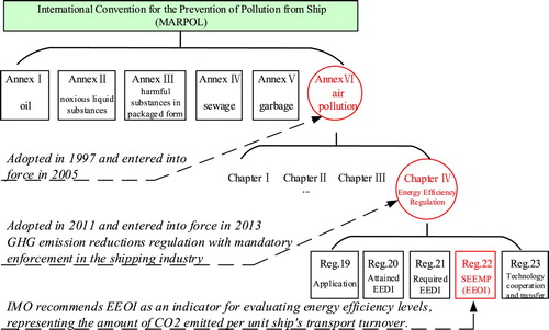
The formula suggested by the IMO for calculating the EEOI for one voyage is presented as (IMO 2009): (1) $EEOI=\frac{\sum _{j}F{C}_j\times C_{Fj}}{m_{c\arg o}\times D}$(1) where $j$ represents the fuel type; $F{C}_j$ is the total fuel consumption on the voyage (tonnes); $C_{Fj}$ is the carbon content of the fuel $j$; $m_{c\arg o}$ is the amount of cargo transported (tonnes); and $D$ is the voyage distance (nautical miles).

3. Data collection and feature analysis

Physical aspects of the selected ship, data capture and measurement uncertainty etc. will be detailed.

3.1. Introduction of selected ship and onboard data collection

A Chinese coastal bulk carrier is selected for the case study. This Handymax bulk carrier is one of the three principal ship types in the present shipping market. Figure 2 shows the selected ship and its route.

Figure 2. Bulk carrier and its route. (a) selected ship. (b) Chinese coastal water.

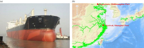
In Figure 2(b), the green scatter details the real-time position of the ships sailing in these Chinese coastal waters; the red line is the route of the selected ship. This coastal area is very busy in shipping activity, where:

• 6 or 7 of the world’s top-10 ports are located;

• 6 million ship voyages are completed every year (Zhao 2016);

• 16% of global shipping CO₂ emissions are produced in east Asia waters (Liu et al. 2016).

Additionally, as these coastal areas are in close proximity to China's large population centres, air pollution from ships and ports can pose significant public health risks. This gives the study of ship energy efficiency of coastal cargo shipping added significance.

To obtain the real-time data, a data collection system has been developed to capture and record the data from sensors at a frequency of one sample per second. For the details of the monitoring and communication refer to (Fan et al. 2016). The detailed information of the selected ship as well as the collected parameters are shown in Table 1 and Figure 3.

Figure 3. Key data collection sensors. (a) Fuel meter. (b) Power meter.

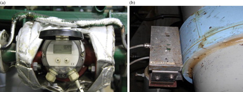
Table 1. Ship parameters and collected parameters.

Length	190 m	Breadth	32.26 m
Main engine	Man B&W 6S50MC	Fuel type	IFO 380
Rated power	9480 kW	Rated speed	127 rpm
GWT	53,000 tonne	Scantling draft	12.5 m
Sensors	Collection parameters
Fuel meter	Real-time fuel consumption$fc$, already mounted on the pipeline of the service tank (Type: volumetric meter; accuracy level: +/- 0.5%)
Shaft power meter	Real-time shaft power $P_D$, already mounted on the tail shaft (Type: strain gauge; accuracy level: +/- 0.5%)
Other collected parameters: ship speed over ground and water, main engine revolution speed, wind speed, water depth, trim etc.

3.2. Uncertainty and feature analysis of measured data

There exists some uncertainties in onboard data collection due to the impact of many factors, including the harsh environment and a degree of inherent uncertainty of the sensors. More specifically:

(1)

Uncertainty caused by environmental factors. The environmental factors can include: Temperature affects on fuel consumption monitoring. On the selected ship, measurement of fuel consumption is based on a volumetric meter. Temperature will inevitably affect the measured value of the ship fuel consumption, especially when the fuel temperature varies significantly en route. Electromagnetic interference affects communication. The complicated ambient electromagnetic environment will affect the signal transmission, especially for parameters using wireless communication, such as shaft power, GPS, etc. According to past experience, when the ship sails into communication control areas, e.g. military docks and hydroelectric dams, shaft power and GPS signals are often blocked or suffer interference, resulting in abnormal data. Obstructions affect communication. Rainy and cloudy weather, mountains, ship hulls and other obstacles will have an adverse impact on GPS communications.

(2)

Inherent uncertainty of sensors. Inherent uncertainty exists in all sensor based monitoring. This type of uncertainty due to system errors of sensors are difficult to avoid. It can be reflected in the accuracy level of the sensor. Generally, the higher the precision of the sensor, the smaller the uncertainty.

Due to the impact of the above-mentioned uncertainty factors, singular points, e.g. zero, negative or outliers, exist in different data parameters even though the selected sensors have a relatively high level of accuracy. Therefore, the measured data needs to be preprocessed before analysis, including recognition and removal of singular points. For detailed procedures of the data preprocessing refer to (Yin and Zhao 2017).

To reduce the computational complexity, the original data are further numbered and sampled at set intervals, as shown in Figure 4. These real-time data can be used to analyse the ship’s operational profiles. In the meantime, the data can help the manager calculate the ship’s EEOI as well as verify the research model.

Figure 4. Measured data trend over a whole voyage.

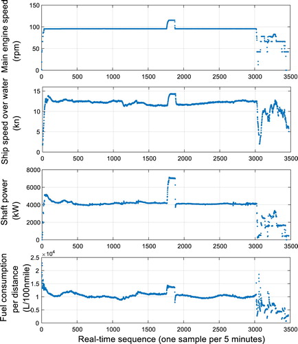
Figure 4 presents the real-time data of engine speed, ship speed, power and fuel consumption over a whole voyage, which is southbound journey with the ship fully loaded. It shows:

• the engine speed was kept at a near constant 96 rpm for most of the voyage.

• although the engine speed shows minimal variation, the ship’s speed, power output, and fuel consumption change continuously due to the impact of multiple internal and external factors on the ship’s fluid dynamic resistance, such as sea state, weather, waterway scale, ship trim and rudder movement.

In the next section, multiple factors will be considered and taken into account, such as environmental parameters, cargo loading, and ship speed. An energy efficiency model will be developed for the selected ship.

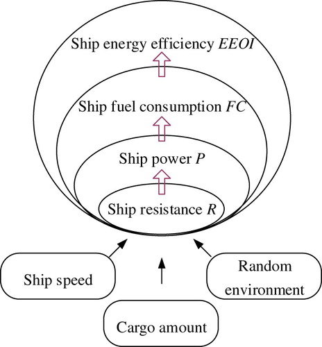
4. Modelling of ship energy efficiency

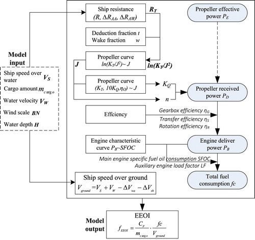
The ship energy efficiency model includes the following sub-models: Ship EEOI, ship fuel consumption, ship power and ship fluid dynamic resistance (hereafter referred to as ship resistance). Figure 5 details the relationship among external factors and ship resistance, power, fuel consumption and energy efficiency.

Figure 5. Interaction among external factors and ship energy efficiency.

4.1. Ship EEOI model

In Equation (1)(1) $EEOI=\frac{\sum _{j}F{C}_j\times C_{Fj}}{m_{c\arg o}\times D}$(1) , both the fuel consumption and the voyage distance are accumulated variables, indicating the integration of the instantaneous variables in the time dimension. Equation (1)(1) $EEOI=\frac{\sum _{j}F{C}_j\times C_{Fj}}{m_{c\arg o}\times D}$(1) can be represented as (2) $EEOI=\frac{C_F}{m_{c\arg o}}\cdot \int \frac{fc\cdot t}{V_{ground}\cdot t}\text{d}t$(2) where $fc$ indicates the ship real-time fuel consumption; $t$ indicates the voyage time; $V_{ground}$ indicates the ship speed over ground

To analyse the dynamic characteristics of ship voyage, the dynamic expression of EEOI can be obtained by differentiating the Equation (2)(2) $EEOI=\frac{C_F}{m_{c\arg o}}\cdot \int \frac{fc\cdot t}{V_{ground}\cdot t}\text{d}t$(2) with respect to time (Fan et al. 2015). (3) $f_{EEOI}=d\left(EEOI\right)=\frac{C_F}{m_{c\arg o}}\cdot \frac{fc}{V_{ground}}$(3) In the actual ocean environment, the wind, wave, shallow water and current could result in involuntary speed loss.

The speed loss due to wind and wave $\mathrm{\Delta }{V}_{wa}$ can be represented by (Kwon 2008): (4) $\left\{\begin{array}{l}\frac{\mathrm{\Delta }{V}_{wa}}{V_S}100\mathrm{\%}=C_{\beta }{C}_U{C}_{Form}\\ \mathrm{\Delta }{V}_{wa}=V_S-V_S^{\mathrm{\prime }}\\ V_S=F_n\sqrt{L_{pp}g}\end{array}\right.$(4) where $V_S$ is the ship speed in calm water; $V_S^{\mathrm{\prime }}$ is the ship speed under the selected weather conditions; $C_{\beta }$ is the speed direction reduction coefficient, which is dependent on the direction of the weather and the Beaufort number BN; $C_U$ is the speed reduction coefficient, which is dependent on ship’s block coefficient $C_B$, the loading conditions and the Froude number $F_n$; $C_{Form}$ is the hull form coefficient, which is dependent on the ship type, the BN and the ship displacement.

The loss due to shallow water $\mathrm{\Delta }{V}_{sh}$ can be represented by (Lackenby 1963): (5) $\frac{\mathrm{\Delta }{V}_{sh}}{V_S}=0.1242\left(\frac{A_M}{h^2}-0.05\right)+1-{\left(\tanh \frac{gh}{{V_S}^2}\right)}^{1/2}$(5) where $A_M$ is the transverse projected area under the waterline; $h$ is the water depth.

Based on Equations (4) and (5), the ship speed over ground can be represented by (6) $V_{ground}=V_S+V_W-\mathrm{\Delta }{V}_{wa}-\mathrm{\Delta }{V}_{sh}$(6) where $V_W$ indicates the water velocity, if the ship sails against the current, $V_W$ would be negative.

4.2. Ship fuel consumption model

For the selected ship, only the main and auxiliary engines are at work while the ship is at sea. Thus, the fuel consumption of the ship is $fc=MEfc+AEfc$, where $MEfc$ indicates the fuel consumption of the main engine, which is dependent on the propulsion load of the ship; normally $MEfc=P_{\mathrm{B}}\cdot SFOC$, where $P_{\mathrm{B}}$ indicates the delivered power of the main engine, $SFOC$ indicates the specific fuel oil consumption of the main engine. For a cargo ship, the fuel consumption of the auxiliary engine is proportional to that of the main engine (Moreno-Gutiérrez et al. 2015). Normally $AEfc=MEfc\cdot LF$, where $LF$ indicates the load factor. As a result, $fc=P_{\mathrm{B}}\cdot SFOC(1+LF)$.

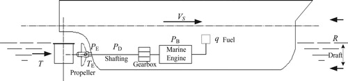
4.3. Main engine power model

4.3.1. Interaction of ship-engine-propeller

The ship propulsion system is essentially an energy transformation system composed of the hull-engine-propeller. Their interactions are simplified and depicted in Figure 6. The power delivered by the main engine $P_B$ needs to be transmitted via a speed reduction gearbox (if fitted), propeller shaft and other transmission components (bearings etc.). Due to the inherent frictional losses, the power delivered to the propeller $P_D$ is less than $P_B$. The power received by the propeller is itself converted to effective power $P_E$ after the interaction of the water with the propeller and hull.

Figure 6. Schematic diagram of the hull-engine-propeller system.

The relationship between $P_B$ and $P_E$ can be represented by (7) $P_B=P_{\mathrm{E}}/{\eta }_S{\eta }_G{\eta }_O{\eta }_H{\eta }_R$(7) where ${\eta }_S$ indicates shaft transfer efficiency; ${\eta }_G$ indicates gearbox efficiency; ${\eta }_O$ indicates open water propeller efficiency; ${\eta }_R$ indicates relative rotation efficiency; ${\eta }_H$ indicates hull efficiency, normally ${\eta }_H=(1-t)/(1-w)$, where $t$ indicates thrust deduction fraction and $w$ indicates wake fraction.

When the ship is at sea, the hull will encounter resistance $R$ from the water. To overcome this resistance and maintain the ship’s speed, the main engine needs to produce a certain amount of power $P_B$ (through burning a certain amount of fuel $MEfc$) to rotate the propeller, generating a thrust force $T$ that propels the ship forward.

When the ship sails at constant speed $V_S$, the total effective thrust force $T_E$ generated by the propeller equals the total resistance of the ship $R$: (8) $R=T_E=(1-t)T$(8) The effective power generated by the propeller $P_E$ can be represented by (9) $P_E=T_E{V}_S=R{V}_S$(9)

The thrust force of the propeller can be calculated by (10) $T=K_T\rho n^2{D}^4$(10) The open water propeller efficiency ${\eta }_O$ can be calculated by (11) ${\eta }_0=\frac{K_T}{K_Q}\cdot \frac{J}{2\pi }$(11)

The advance coefficient of the propeller $J$ can be calculated by (12) $J=\frac{V_A}{nD}=\frac{(1-w)\cdot V_S}{nD}$(12) According to Equations (4)–(9), $P_B$ can be represented by (13) $P_B=\frac{2\pi \rho D^5{n}^3{K}_Q}{{\eta }_S{\eta }_G{\eta }_R}$(13) where $K_T$ is the thrust coefficient; $V_A$ is the advance speed of the propeller; $K_Q$ is the torque coefficient; $\rho$ is the water density; $n$ is the shaft revolution speed; $D$ is the propeller diameter.

4.3.2. Propeller open water characteristic

The open water characteristic curves are required to calculate the torque coefficient $K_Q$. For the selected ship, the number of propeller blades $Z=4$, the blade area ratio $A_E/A_O=0.53$, and the pitch ratio $P/D=0.74$. The open water characteristic of the propeller (MAU4-53, $P/D=0.74$) is obtained through the interpolation to the propeller map, as shown in Figure 7.

Figure 7. Propeller open water characteristic curves.

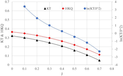
Using the characteristic curves in Figure 7, the calculation of $K_Q$ and $n$ is shown as follows:

1. 1. $\ln \left(K_T/J^2\right)$ is first calculated by $K_T/J^2=R/\left[\rho (1-t){(1-w)}^2{V_S}^2{D}^2\right]$, which can be obtained from Equations (8)–(12). The advance coefficient $J$ can be obtained by interpolation of the curve $J\sim \ln \left(K_T/J^2\right)$, as shown by the blue curve in Figure 7. Similarly, the torque coefficient $K_Q$ can be obtained by interpolation of the curve $J\sim 10K_Q$, as shown by the red curve in Figure 7.

2. 2. The propeller revolution speed $n$ can be obtained using Equation (12)(12) $J=\frac{V_A}{nD}=\frac{(1-w)\cdot V_S}{nD}$(12) .

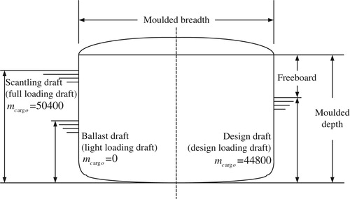
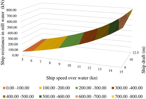
4.4. Ship resistance model

For a cargo ship, the deeper the draft, the greater the ship resistance and therefore the greater the power required from the main engine to attain the same transit speed. Figure 8 presents the typical ship drafts.

Figure 8. Typical drafts of the ship.

The selected ship’s resistance characteristics corresponding to the three drafts are calculated in accordance with the Holtrop-Mennen method (Holtrop and Mennen 1982). This method presents that a ship’s total resistance in still water $R$ can be represented: (14) $R=R_F(1+k_1)+R_{APP}+R_W+R_B+R_{TR}+R_A$(14) where $R_F$ indicates frictional resistance; $1+k_1$ indicates form factor describing the viscous resistance of the hull form in relation to $R_F$; $R_{APP}$ indicates resistance of appendages; $R_W$ indicates wave-making and wave-breaking resistance; $R_B$ indicates additional pressure resistance of the bulbous bow near the water surface; $R_{TR}$ indicates additional pressure resistance of immersed transom stern; $R_A$ indicates model-ship correlation resistance.

According to the ITTC-1957 friction formula, frictional resistance $R_F$ can be calculated by (15) $R_F=0.5C_f\rho S{V}_S^2$(15) where $C_f$ is the frictional resistance coefficient, which can be determined by $C_f=0.075/{(\log R_n-2)}^2$, where Reynolds number $R_n=V_{S}L/\gamma$; $S$ is the wetted area of the hull.

Form factor of the hull $1+k_1$ can be calculated by (16) $\begin{array}{rl}1+k_1& =C_{13}\{0.93+C_{12}{\left(B/L_R\right)}^{0.92497}\\ & \times {(0.95-C_P)}^{-0.521448}\\ & \times {(1-C_P+0.0225lcb)}^{0.6906}\}\end{array}$(16) where $B$ is the breadth; $L_R$ is the length of the run; $C_P$ is the prismatic coefficient; $lcb$ is the longitudinal centre of buoyancy.

Wave-making and wave-breaking resistance $R_W$ can be calculated by (17) $R_W=c_1{c}_2{c}_5\mathrm{\nabla }\rho g\exp \left\{m_1{F}_n^d+m_2\cos \left(\lambda F_n^{-2}\right)\right\}$(17) where $\mathrm{\nabla }$ is the displacement volume; $F_n$ is the Froude Number, which can be determined by $F_n=V_S/\sqrt{gL}$.

Model-ship correlation resistance $R_A$ can be calculated by (18) $R_A=0.5\rho {V_S}^{2}S{C}_A$(18) where $C_A$ is the correlation allowance coefficient, which can be determined by

$C_A=0.006(L+100{)}^{-0.16}-0.00205+0.003\sqrt{L/7.5}{C_B}^4{c}_2(0.04-c_4)$, where $C_B$ is the block coefficient.

For the above estimation of the ship resistance, many variables and coefficients are involved. First, the ship’s characteristic parameters, e.g. block coefficient $C_B$, prismatic coefficient $C_P$, and so on; the values of which are based on the selected ship. Second, regression parameters, e.g. $m_i$ and $c_i$, the values of which are determined in accordance with previous research (Holtrop and Mennen 1982; Rakke 2016).

Based on the Equations (14)–(18), the ship still water resistance under different speeds and drafts can be estimated, as shown in the three-dimensional Figure 9.

Figure 9. Ship resistance characteristics in still water.

The environmental parameters are believed to have a certain impact on ship’s resistance (Fan, Yan, Yin 2017), therefore, the wind and wave loads need be considered.

The wind resistance can be calculated by (Andersen 2013): (19) $\mathrm{\Delta }{R}_{AA}=C_X\cdot \frac{1}{2}{\rho }_A{V}_A^2{A}_T$(19) where $C_X$ is the wind force coefficient; ${\rho }_A$ is the density of the air; $V_A$ is the relative wind speed and $A_T$ is the transverse projected area above the waterline.

The additional wave resistance can be calculated by (ITTC 2005): (20) $\mathrm{\Delta }{R}_{AW}=0.64{{\xi }_W}^2{B}^2{C}_B\rho g/L$(20) where ${\xi }_W$ is the wave height; $B$ is the ship width; $C_B$ is the block coefficient; $\rho g$ is the sea water specific gravity; $L$is the ship length.

With regard to Equations (19)(19) $\mathrm{\Delta }{R}_{AA}=C_X\cdot \frac{1}{2}{\rho }_A{V}_A^2{A}_T$(19) and (20)(20) $\mathrm{\Delta }{R}_{AW}=0.64{{\xi }_W}^2{B}^2{C}_B\rho g/L$(20) , the relative wind speed $V_A$ and wave height ${\xi }_W$ are both associated with the natural true wind, which is usually scaled by Beaufort number (BN). Therefore, $V_A$ and ${\xi }_W$ would be represented by a common variable BN in the simulation.

5. Simulation and verification of ship energy efficiency

Simulated calculations will be carried out based on the above-mentioned ship energy efficiency model. The model will be verified using both the simulated and measured data collected in the southbound journey under full loading draft.

5.1. Simulated calculation

The flow chart of the simulated calculation is shown in Figure 10.

Figure 10. Flow chart of simulated calculation of EEOI.

The specific procedures are as follows:

• (1) Generation of the input parameters $V_S$, $m_{c\arg o}$, $V_W$, BN, and H.

According to Section 4.4, there are three possible values for $m_{c\arg o}$, which are 0, 44800, and 50400 respectively. With regard to the southbound journey, the ship is fully loaded, thus $m_{c\arg o}$=50400 here. As the ocean current speed, wind speed, and water depth are environmental variables with a high degree of uncertainty and randomness, in this paper, they are regarded as random variables. The Monte Carlo simulation method is used to realise the fusion of these input parameters and the energy efficiency model.

More specifically:

• Construct and describe the probability distribution of the random variables;

• Generate samples randomly into the model from the probability distribution.

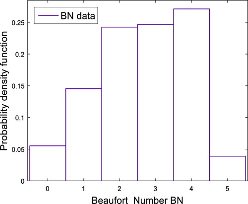
To obtain the distribution characteristics of these random environmental variables, the measured data of the southbound voyage, i.e. fully loaded, is statistically analysed. Figures 11 and 12 are the probability distribution and kernel density estimation (KDE) of $V_W$ and H. Figure 13 is the probability distribution of BN, which is obtained from the measured data of wind speed in accordance with Beaufort wind scale (Barua 2005). Here, BN is a discrete random variable.

Figure 11. Water velocity probability distribution and estimation.

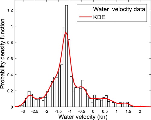
Figure 12. Water depth probability distribution and estimation.

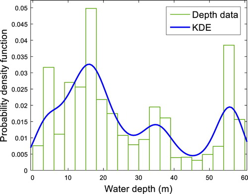
Figure 13. Beaufort wind scale probability distribution.

Table 2 presents the details of the Monte Carlo simulation.

(2)

Section 4.3.2 details how the corresponding advance coefficient $J$, torque coefficient $K_Q$, and revolution speed n can be obtained; Section 4.3.1 details how the corresponding power delivered by the main engine $P_B$ can be obtained; Section 4.2 details how the corresponding specific fuel oil consumption $SFOC$, main engine fuel consumption $MEfc$ and auxiliary engine fuel consumption $AEfc$ can be obtained; finally, in accordance with Section 4.1, the ship EEOI can be calculated.

Table 2. Monte Carlo simulation of the random input parameters.

Input parameters	Probability distribution satisfied	Random number generation method	MATLAB/Simulink realisation module
Ship speed over water $V_S$	Obeys uniform distribution $V_S$∼U [5,15]	Direct generation	Uniform Random Number
Water velocity $V_W$	Obeys the distribution shown in Figure 11.	Inverse transform method	Uniform Random Number and 1-D Lookup Table module
Water depth $H$	Obeys the distribution shown in Figure 12.	Inverse transform method	Uniform Random Number and 1-D Lookup Table module
Beaufort number$BN$	Obeys the distribution shown in Figure 13.	–	Uniform Random Number module

Note: Inverse transform method indicates generating random numbers from any probability distribution given its inverse CDF (Gentle 2006; Fan, Yan, Yin 2017).

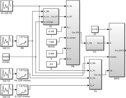
The calculation procedures can be realised on the MATLAB/Simulink platform, as shown in Figure 14.

Figure 14. Ship energy efficiency Simulink model.

Using this Simulink model, the simulated results aimed at full loading draft can be obtained, as shown in Figures 15,16 and 17.

Figure 15. Comparison between the measured and simulated data.

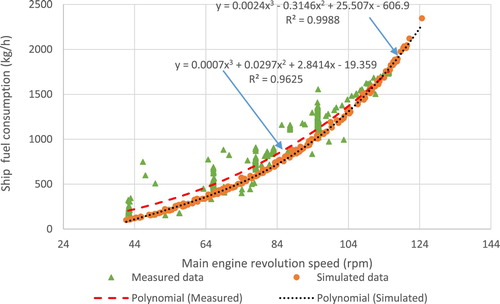
Figure 16. Simulated ship speed and environmental parameters.

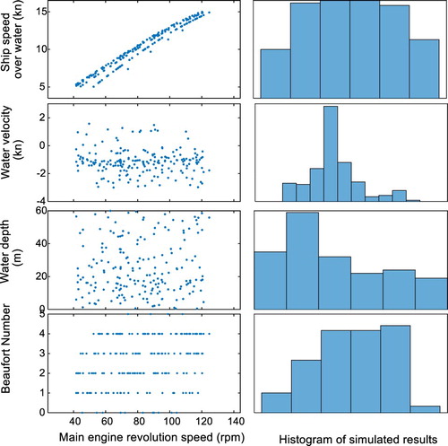
Figure 17. Comparison of the EEOI under different loading conditions.

5.2. Model verification

To evaluate the accuracy of the model, the measured fuel consumption data collected during the full load voyage were compared with the simulated results, as shown in Figure 15.

In Figure 15, the X-axis is the main engine revolution speed, and the Y-axis is the ship fuel consumption. The orange scatter are the simulated results, and the green scatter are the measured data. It indicates the measured data shows a discrete distribution. The main reason for the dispersion are the changeable working conditions of the ship. Specifically, in the actual sailing, the operating conditions of the ship will change continuously, such as sea conditions, weather, waterway scale, fouling and rudder movement, all of which could result in change of ship resistance; as a result, the ship fuel consumption would change in accordance; in other words, the ship fuel consumption is an interval value corresponding to each engine speed.

As the measured data is scattered, comparative verification is carried out based on statistical methods. First, the measured and simulated data in Figure 15 are regressed. Correspondingly, the red and black regression curves are obtained as well as the regression equation and R² value. Then, by selecting several revolution speeds, values of the two regression equations are calculated. Their differences are calculated to evaluate the accuracy of the model. With regard to the commonly used speed range (76–116) rpm, the average difference of the two regression equations is in the region of 6.46%, which indicates that the established model has good accuracy.

6. Results and discussion

Figure 16 presents the simulated ship speed and environmental parameters.

In Figure 16, the X-axis is the main engine revolution speed, the Y-axes are the ship speed over water, current speed, water depth, and Beaufort number respectively. From the scattered distributions in the left hand traces, it is clear that the simulated ship speed, which is affected by random environmental parameters, is also an interval value corresponding to each revolution speed. The histograms of the environmental parameters show almost identical distribution features with that in Figures 11,12, and 13. This confirms the proposed Monte Carlo simulation method can simulate the random characteristics of the real environmental parameters.

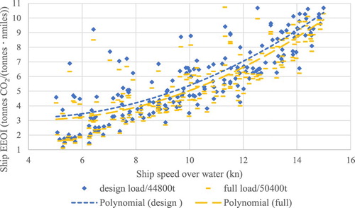
Figure 17 presents the simulated EEOI of the selected ship under design and full loading conditions. The X-axis is the ship speed over water; and the Y-axis is the EEOI. As detailed by the regression curves, the ship EEOI increases with increasing ship speed. Under the same speed conditions, the less cargo loaded, the higher the EEOI. Furthermore, the EEOI of the design load is about 6.44% higher than that at full load on average.

In summary, the relationship between the ship EEOI, fuel consumption, cargo loading, ship speed and environmental variables can be described as:

1. The amount of cargo determines the ship’s draft. For the same ship speed, the more cargo loaded, the higher the ship’s fuel consumption and lower EEOI is attained.

2. Under a specific loading condition, the main engine revolution speed is the main influencing factor of the ship fuel consumption, the growth rate of which whose growth rate increases with increasing shaft revolution speed.

3. The random environmental parameters, including wind, wave, and shallow water, impact on the ship’s fuel consumption and the EEOI.

4. As a result of the effect of random environmental parameters, for a specific ship draft and speed, the measured rate of the ship fuel consumption and the EEOI show discrete and interval values.

7. Conclusions

Ship energy efficiency is influenced by many factors. These include the cargo loading, the ship’s speed, and the random environmental influences (wind, current, wave, waterway depth, etc.). With consideration of the random nature of the environmental parameters, a novel ship energy efficiency model was developed and used to simulate ship performance. The actual ship’s data with a range of loadings, speeds and available environmental conditions during data condition were used to verify the model, which indicates that the model demonstrates good accuracy. In general, the devised model can simulate the ship energy efficiency under different loading conditions, ship speed and sea state. This study is beneficial to the ship manager to assess ship energy efficiency at sea, and to provide decision support for optimising ship energy efficiency, which is beneficial for promoting the energy saving and emission reduction within the shipping industry.

Acknowledgements

Special thanks and appreciation go to the chief engineer of the bulk carrier, Jiahehangyun 1, who supports a lot in providing the necessary ship information and the noon report data. Sincere appreciation goes to Konrad Yearwood, who gave valuable advice towards improving this paper.

Disclosure statement

No potential conflict of interest was reported by the authors.

ORCID

Xinping Yan http://orcid.org/0000-0002-2265-2689

Additional information

Funding

This work was supported by the High-tech Ship Programme from Ministry of Industry and Information Technology of China (2014502), the National Natural Science Foundation of China (51809202), and the Fundamental Research Funds for the Central Universities (2016-YB-022).

References

- Aldous L, Smith T, Bucknall R, Thompson P. 2015. Uncertainty analysis in ship performance monitoring. Ocean Eng. 110(6):29–38. doi: 10.1016/j.oceaneng.2015.05.043
- Andersen IMV. 2013. Wind loads on post-panamax container ship. Ocean Eng. 58(2):115–134. doi: 10.1016/j.oceaneng.2012.10.008
- Banawan AA, Mosleh M, Seddiek IS. 2013. Prediction of the fuel saving and emissions reduction by decreasing speed of a catamaran. J Mar Eng Technol. 12(3):40–48.
- Barro RDC, Kim J, Lee D. 2010. Real Time Monitoring of Energy Efficiency Operation Indicator on Merchant Ships. J Korean Soc Mar Eng. 33:40–45.
- Barua DK. 2005. Beaufort wind scale. Encyclopedia of coastal science. Netherlands: Springer; p. 186–186.
- Bocchetti, D., Lepore, A., Palumbo, B., Vitiello, L. 2015. A statistical approach to ship fuel consumption monitoring. J Ship Res. 59(3). doi:10.5957/JOSR.59.3.150012.
- Bowslarkin A, Anderson K, Mander S, Traut M, Walsh C. 2015. Shipping charts a high carbon course. Nat Clim Change. 5(4):293–295. doi: 10.1038/nclimate2532
- Coraddu A, Figari M, Savio S. 2014. Numerical investigation on ship energy efficiency by Monte Carlo simulation. P I Mech Eng M-J Eng. 228(3):220–234.
- Fan A, Yan X, Yin Q. 2015. [Energy efficiency model of marine main engine]. J Traffic Transp Eng. 15(4):69–76. Chinese.
- Fan A, Yan X, Yin Q. 2016. A multisource information system for monitoring and improving ship energy efficiency. J Coast Res. 32(5):1235–1245. doi: 10.2112/JCOASTRES-D-15-00234.1
- Fan A, Yan X, Yin Q. 2017. Modeling and analysis of ship energy efficiency operational indicator based on the Monte Carlo method. Nav Eng J. 129(1):87–98.
- Fan A, Yan X, Yin Q, Zhang D. 2017. Clustering of the inland waterway navigational environment and its effects on ship energy consumption. P I Mech Eng M-J Eng. 231(1):57–69.
- Gentle JE. 2006. Random number generation and Monte Carlo methods. New York: Springer Science & Business Media.
- Holtrop J, Mennen GG. 1982. An approximate power prediction method. Int Shipbuild Prog. 335(29): 166–170. doi: 10.3233/ISP-1982-2933501
- [IMO] International Maritime Organization. 2009. Guidelines for voluntary use of the ship energy efficiency operational indicator (EEOI). MEPC.1/Circ.684. London: Marine Environment Protection Committee.
- [IMO] International Maritime Organization. 2011. Report of the Marine Environment Protection Committee on its sixty-second session. London: Marine Environment Protection Committee.
- [ITTC] International Towing Tank Conference. 2005. Full scale measurements – speed and power trials – analysis of speed/power trial data. Edinburgh: Recommendations of the 24th ITTC.
- Ji M, Shen L, Shi B. 2015. [Routing optimization for multi-type containerships in a hub-and-spoke network]. J Traffic Transp Eng. 2(5):362–372. Chinese.
- Kwon YJ. 2008. Speed loss due to added resistance in wind and waves. Nav Archit. 3:14–16.
- Lackenby H. 1963. The effect of shallow water on ship speed. Shipbuild Mar Eng. 70:446–450.
- Liu H, Fu M, Jin X, Shang Y, Shindell D, Faluvegi G, Shindell C, He K. 2016. Health and climate impacts of ocean-going vessels in East Asia. Nat Clim Change. 6(11):1037–1041. doi: 10.1038/nclimate3083
- Meng Q, Du Y, Wang Y. 2016. Shipping log data based container ship fuel efficiency modeling. Transp Res B-Meth. 83:207–229. doi: 10.1016/j.trb.2015.11.007
- Moreno-Gutiérrez J, Calderay F, Saborido N, Boile M, Valero RR, Durán-Grados V. 2015. Methodologies for estimating shipping emissions and energy consumption: a comparative analysis of current methods. Energy. 86:603–616. doi: 10.1016/j.energy.2015.04.083
- Osses JRP, Bucknall RWG. 2014. A marine engineering plant model to evaluate the efficiency and CO2 emissions from crude oil carriers. Shipping in Changing Climates: Provisioning the Future Conference; Liverpool.
- Rakke SG. 2016. Ship emissions calculation from AIS [dissertation]. Trondheim: Norwegian University of Science and Technology.
- Smith TWP, Jalkanen JP. 2014. Third IMO GHG study 2014. London: IMO; p. 32.
- Tillig F, Ringsberg JW, Mao W, Ramne B. 2017. A generic energy systems model for efficient ship design and operation. P I Mech Eng M-J Eng. 231(2):649–666.
- Trodden DG, Murphy AJ, Pazouki K, Sargeant J. 2015. Fuel usage data analysis for efficient shipping operations. Ocean Eng. 110:75–84. doi: 10.1016/j.oceaneng.2015.09.028
- [UNFCCC] United Nations Framework Convention on Climate Change. 2015. http://www.cop21.gouv.fr/en/.
- Vrijdag A. 2014. Estimation of uncertainty in ship performance predictions. J Mar Eng Tech. 13(3):45–55. doi: 10.1080/20464177.2014.11658121
- Wan Z, Zhu M, Chen S, Sperling D. 2016. Pollution: three steps to a green shipping industry. Nature. 530(7590):275.
- Xing S, Xinping Y, Bing W, Xin S. 2013. Analysis of the operational energy efficiency for inland river ships. Transp Res D-Tr E. 22: 34–39.
- Yan X, Sun X, Yin Q. 2015. Multiparameter sensitivity analysis of operational energy efficiency for inland river ships based on backpropagation neural network method. Mar Technol Soc J. 49:148–153. doi: 10.4031/MTSJ.49.1.5
- Yin Q, Zhao G. 2017. [A study on data cleaning for energy efficiency of ships]. J Transp Info Saf. 35(3):68–73. Chinese.
- Zhao P. 2016. [Study on capacity building of the safety supervision on the central government duty waters]. China Mar. 1: 32–36. Chinese.