Study on dynamic slope angle of sandy seabed around the submarine piggyback pipeline in steady flow

Abstract

Submarine piggyback pipeline is an important tool for oil and gas transport, especially, in the marginal oil field. When the scour happens in the seabed, the pipeline slides easily, which may cause the pipeline failure. The dynamic slope angle is one of the most important characteristics of the scour. In this work, the dynamic slope angles of the sandy seabed under piggyback pipelines in steady flow are investigated experimentally and numerically in detail. The physical experiments are conducted in an annular flume and the numerical simulations are carried out using a two-phase flow model which is resolved by the finite volume method (FVM). In the numerical model, the free surface is tracked by the volume of fluid (VOF), and both bed and suspended loads are considered in the scour module. Depending on the comparison and convergence analysis, the numerical results are in good agreement with the experimental results. The results indicate that the dynamic slope angle is significantly affected by the incoming flow velocity, gap-ratio, spacing-ratio and pipe diameter. With the reduction of gap-ratio and space-ratio, the upstream dynamic slope angle α increases slightly, but the downstream dynamic slope angle β decreases. With the increase of the grain Reynolds number, the angle α increases slightly, but the angle β decreases severely. The conclusions drawn from this paper could provide the reference for the design of submarine piggyback pipeline.

1. Introduction

In the marine marginal oil field, submarine piggyback pipeline has been used widely in recent years because this pipeline can solve the problem of the crude oil solidification when the submarine gas and oil are transported. These pipelines are often strapped together and laid on the seabed as a bundle. The bundled pipelines may either be touched with each other or be separated by small gaps. The most popular structure of the bundled pipelines consists of one (main) pipe with a large diameter and one pipe with a small diameter. In the next paper, the small diameter pipe of the bundled pipeline is abbreviated as small pipe. The two-pipe configuration is often referred to as submarine piggyback pipeline in the oil and gas industry (Zhao and Cheng 2008; Zang et al. 2013, 2018).

When the submarine pipeline is laid on the seabed, the disturbance flow caused by the laying pipeline can induce local scour around the pipeline. A local scour can cause the suspension of pipeline, which is the potential danger for the pipeline damage. Hence, many investigations about the interaction between the seabed and the submarine pipeline have been carried out to reveal the mechanism of the local scour around the submarine pipeline. Chiew (1990) experimentally observed the detailed phenomenon of the local scour around a submarine pipeline and revealed that the piping and the stagnation eddy combine to induce the onset of scour and undermine the pipeline. Sumer et al. (1988) did an experiment about the effect of lee-wake on scour below pipelines in flow and showed that the downstream scour of the pipe is apparently governed by the action of an organised wake flow, which is a series of agglomeration of large-scale vortices. Dey and Singh (2007) presented a semi-theoretical model for the computation of maximum clear-water scour depth below submarine pipelines in uniform sediments under steady flow, and the results showed that the maximum scour depth below pipelines with upward seepage through the bed is smaller than that without seepage. So far, many studies have been carried out on the submarine single pipeline (Zhao, Shi, et al. 2015; Yang et al. 2012).

However, there are only a few researches about the piggyback pipeline published, let alone the scour around it (Zhao et al. 2018). Local scour around a piggyback pipeline in steady flow was investigated numerically by Zhao and Cheng (2013). They found the flow fields and scour profiles are significantly influenced by the gap ratio. Nevertheless, this finding has not yet been verified through an experiment. A series of experiments about the vibration of piggyback pipelines induced by steady flow close to a plane seabed were conducted by Zang and Gao (2014) with a hydro-elastic facility in a conventional water flume. The effect of the mass-damping parameter, diameter ratio, gap-to-diameter ratio, the spacing-to-diameter ratio and the position angle on the VIV (Vortex-Induced Vibration) response was studied. The results showed that the peak vibration amplitude of near-wall piggyback pipelines is smaller than that for a wall-free single pipeline. Cheng et al. (2013) researched the influence of proximity of the seabed on hydrodynamic forces on submarine piggyback pipelines under wave action, and this research did not consider the scour around a piggyback pipeline.

In order to study the local scour around the piggyback pipeline particularly, the research is carried out experimentally and numerically and presented in this paper. During the evolution of the scour hole around a submarine pipeline, slope angle plays a significant role in determining the profile of the scour hole. When the slippage of pipeline happens in the scour hole, the pipeline is prone to buckling failure. Therefore, it is necessary to study the slope angle of the scour hole under the submarine piggyback pipeline. When the evolution of the scour approaches to the state of equilibrium, the profile of scour hole remains unchanged. The angle between the hole surface and the horizontal level is called dynamic slope angle. It is discovered that if the scour hole is formed in the dynamic water environment, the dynamic slope angle is much different from static slope angle which has been studied in many papers (Zhou et al. 2002; Yang et al. 2009). However, few researches have been carried out about the dynamic slope angle. Based on the uniform sediment wedge-shape deposition model, the formulas of the dynamic slope angle for the cohesive and non-cohesive sediment are developed by Huang et al. (2008). Yang et al. (2012) studied the dynamic slope angle of sandy seabed under the submarine spoiler pipeline, and a series of tests were carried with different gaps between seabed and pipeline in unidirectional flow. The research showed that, for a pipe with a spoiler, the upstream dynamic slope angle increases slightly as the increase of the grain Reynolds number, and there is a corresponding reduction in the downstream dynamic slope angle. With the increase of the spoiler height, the trend is more and more obvious.

This study focuses on the dynamic slope angle of sandy seabed around a submarine piggyback pipeline. Due to the existence of small pipe, the local scour of piggyback pipeline differs greatly from that of normal single pipeline. Besides, the piggyback pipelines have been widely used in submarine gas and oil exploitation. So, it is important to study the dynamic slope angle of scour hole around the submarine piggyback pipeline. In the present research, a series of experiments were carried out to study the dynamic slope angle in detail. In addition to the corresponding experimental work, a sediment scour model has been developed using a two-phase flow solver, which is employed to analyse the hydrodynamic characteristics of the piggyback pipeline during the evolution process of the scour hole underneath it. The air–water and water-sediment interfaces are captured using the volume of fluid (VOF) method and the moving-mesh method, respectively (Zhao et al. 2019).

The paper is organised as follows. The settings and results of physical experiments are discussed in Section 2. Section 3 shows the numerical simulation. In Section 4, experimental and numerical data are illustrated, furthermore, the change of dynamic slope angles in different conditions is also discussed. Section 5 summaries the paper and lists issues for future research.

2. Physical experiment

2.1. Experiment model

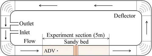
The physical experiments are carried out in River Dynamics Laboratory of Engineering College, Ocean University of China. The length of the annular flume is 25 m. The width and depth of the flume are 0.5 and 0.6 m, respectively. In order to reduce the disturbance of the fluid in the flume, the deflectors are set in the four corners of the flume, as shown in Figure 1. The water flows in the flume at the inlet. When the loop of the flow is formed in the flume, the water flows out at the outlet. At a section of the flume, the sediment is laid flat at the bottom of the flume for the local scour. The length and the height of the sandy bed are 5 and 0.15 m, respectively. The flow velocities are measured using the Acoustic Doppler Velocimeter (ADV). The maximum measuring range of ADV is 4 m/s. And its accuracy is ±1 mm/s. When the scour reaches equilibrium, the profile height of the scour hole is measured using a mechanical measuring pin with a minimum of 0.1 mm.

Figure 1. The experimental setup of annular flume.

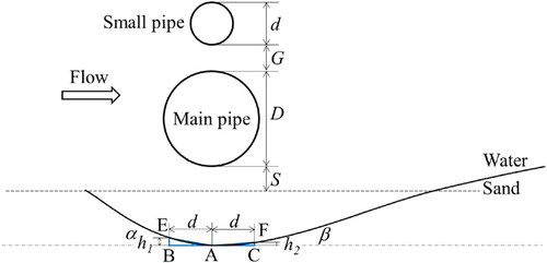
The sketch of piggyback pipeline configuration and local scour is displayed in Figure 2. The pipeline is made by an organic glass tube. The diameters of small pipe and main pipe are denoted as d and D, respectively. G is the gap between the small and main pipes, and S is the spacing between the bottom of main pipe and flat sandy bed. In the scour hole, the slope surface has a curve surface. In order to define the dynamic slope angle, an approximate method is adopted. The deepest point A in the scour hole is extended to the points B and C in the horizontal direction, and the extension distance is d. The vertical lines passing through the points B and C intersect with the slope at the points E and F, respectively. The lengths of BE and CF are h₁ and h₂, respectively. As can be observed in Figure 2, the relationship between the angles and the edges of the triangles ABE and ACF can be expressed as: α = arctan(h₁/d) and β = arctan(h₂/d). α and β are the dynamic slope angles of upstream and downstream, respectively.

Figure 2. The configuration of piggyback pipeline and its local scour.

2.2. Experiment parameters and design

Depending on the engineering practice ratio of the main pipe to small pipe, three different diameters (D) of main pipe are considered as 0.08, 0.10 and 0.12 m, and the diameters (d) of small pipe are set as 0.03, 0.035 and 0.04 m, respectively (Yang et al. 2007). The length of piggyback pipeline is 0.5 m, and the wall thickness is 0.005 m. The gap-ratios e (e = G/D) are set as 0, 0.125, 0.25, 0.375 and 0.5, and the spacing-ratios e₀ (e₀= S/D) are selected as 0, 0.1, 0.2, 0.3, 0.5, 0.7 and 0.9, respectively.

At the beginning of the experiment, the sediment with the particle median diameter of 0.56 mm was laid on the bottom of the flume. The porosity (ζ) of the sediment was 0.39. Then, the piggyback pipeline was supported on the flume using a vertical bracket. Close the inlet and the outlet, and pump the water in the flume using a water pipe. When the water depth from the sandy bed to water surface was 0.4 m, stop injecting water. Both the inlet and the outlet were opened, which induced water flowed circularly in the flume. The water depth and flow velocity were controlled by the discharge of the inlet and the outlet. The water depth was kept at a constant of 0.4 m for all experiments. The flow velocity (u₀) was controlled at 0.24, 0.3 and 0.4 m/s, respectively. To ensure the inflow velocity was satisfied, the velocimeter was located at the middle axes of the main pipe to monitor the velocity, and the distance from the velocimeter to the main pipe center was about 0.5 m (Figure 1). The distance was set before the experiment and measured using the dividing ruler. In the experiment, the water temperature was about 15°C which was measured using a thermometer, and the kinematic viscosity of water at this temperature was 1.1201 × 10⁻⁶m/s². The experiments were performed in the clear-water conditions. The inflow water would not bring the excess sediment to the sandy bed. When the scour reached the equilibrium and the scour hole was unchanged, the scour process of experiment was finished. Close the inlet and the outlet, and drain the flume using the water pump. The profile of the scour hole was measured using the mechanical measuring pin.

The experimental cases and parameters are listed in Table 1 which includes two cases. In case A, the piggyback pipeline is laid on the sand bed directly without spacing-ratio (e₀). The gap-ratio (e) changes from 0 to 0.5. However, only the influence of the gap-ratio (e) on the scour is analysed in case A. In order to analyse the effect of both gap-ratio (e) and space-ratio (e₀) on the scour, case B is designed in the experiment. The gap-ratio (e) is set at 0, 0.25 and 0.5, respectively. The spacing-ratio (e₀) ranks from 0.1 to 0.9.

Table 1. Experimental parameters.

Case	Runs	Main/small pipe diameter (m)	Gap-ratio (e = G/D)	Velocity u0 (m/s)	Spacing-ratio (e0 = S/D)
A	Run 01	0.080/0.030	0/0.125/0.25/0.375/0.5	0.24	0
	Run 02	0.080/0.030	0/0.125/0.25/0.375/0.5	0.30	0
	Run 03	0.080/0.030	0/0.125/0.25/0.375/0.5	0.40	0
	Run 04	0.100/0.035	0/0.125/0.25/0.375/0.5	0.24	0
	Run 05	0.100/0.035	0/0.125/0.25/0.375/0.5	0.30	0
	Run 06	0.100/0.035	0/0.125/0.25/0.375/0.5	0.40	0
	Run 07	0.120/0.040	0/0.125/0.25/0.375/0.5	0.24	0
	Run 08	0.120/0.040	0/0.125/0.25/0.375/0.5	0.30	0
	Run 09	0.120/0.040	0/0.125/0.25/0.375/0.5	0.40	0
B	Run 10	0.120/0.040	0/0.25/0.5	0.24	0.1/0.2/0.3/0.5/0.7/0.9
	Run 11	0.120/0.040	0/0.25/0.5	0.30	0.1/0.2/0.3/0.5/0.7/0.9
	Run 12	0.120/0.040	0/0.25/0.5	0.40	0.1/0.2/0.3/0.5/0.7/0.9

2.3. Experiment results

The investigations of the local scour under the piggyback pipelines with different gap-ratios (e) were conducted, and the scour profiles around the piggyback pipelines with D = 0.10 m are shown in Figure 3.

Figure 3. The scour profiles around the piggyback pipelines with D = 0.10 m. (a) e = 0, u₀=0.3 m/s, (b) e = 0, u₀=0.4 m/s, (c) e = 0.25, u₀= 0.3 m/s, (d) e = 0.25, u₀=0.4 m/s, (e) e = 0.5, u₀=0.3 m/s, (f) e = 0.5 and u₀ = 0.4 m/s.

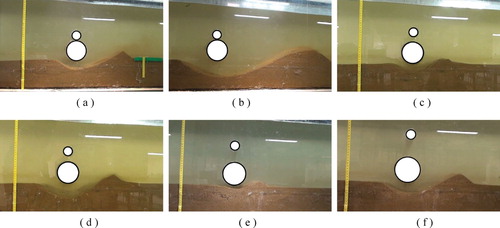
As shown in Figure 3(a,c,e), when the inflow velocity is 0.3 m/s, with the increase of gap-ratio (e), the scour hole becomes smaller and smaller. When both the gap-ratio (e) and spacing-ratio (e₀₎ are zero, the range of scour hole under the same steady flow arrives at the maximum. At the same velocity flow, the upstream dynamic slope angle (α) decreases slightly as the gap-ratio increases. However, with the gap-ratio increasing, the downstream dynamic slope angle (β) remarkably increases. The change of angle β is more serious than that of angle α.

With the increment of fluid velocity, the depth and length of the scour hole increase obviously for the same piggyback pipeline, as shown in Figure 3(a,b). The upstream dynamic slope angle (α) increases slightly as the inflow velocity increases. However, the downstream dynamic slope angle (β) decreases severely with the increase of velocity.

Furthermore, with the decrease of gap-ratio and the increase of fluid velocity, the deepest point of the scour hole moves to the further downstream position. In conclusion, it distinctly indicates that the increment of flow velocity and the reduction of the gap ratio can accelerate scour of the hole, and the dynamic slope angles are impacted by many factors including incoming velocity, pipe diameter and various ratios.

3. Numerical simulation

Except for the physical experiments, the numerical simulations were also conducted to investigate the local scour and the hydrodynamic characteristics around the submarine piggyback pipeline. The computational domain is divided by the unstructured mesh grids.

3.1. Numerical model

3.1.1. Flow module

The flow is solved by Naiver-Stokes equations: (1) $\begin{array}{rl}& \mathrm{\nabla }\cdot \mathbf{u}=0,\end{array}$(1) (2) $\begin{array}{rl}& \frac{\mathrm{\partial }\mathbf{u}}{\mathrm{\partial }t}+\mathrm{\nabla }\cdot \mathbf{(}\mathbf{u}\mathbf{u})\\ & =\mathrm{\nabla }\cdot \left({\nu }_{\text{e}}\mathrm{\nabla }\mathbf{u}\right)+\mathrm{\nabla }\mathbf{u}\cdot \mathrm{\nabla }{\nu }_{\text{e}}-\mathrm{\nabla }\frac{\text{p}}{\rho }+(1-\text{r})\cdot \text{g},\end{array}$(2) where ∇ the gradient operator, u the flow velocity, t the time, ν_e the effective kinematic viscosity, p the pressure, ρ the density, r the ratio of the density to the reference density, g the gravity acceleration.

The turbulent viscosity μ_t is calculated by two-equation κ-ε turbulence model: (3) ${\mu }_{\text{t}}=C_{\mu }\rho \frac{{\kappa }^2}{\epsilon },$(3) (4) $\frac{\mathrm{\partial }\kappa }{\mathrm{\partial }\text{t}}+\mathrm{\nabla }\cdot \left(\mathbf{u}\kappa \right)=\frac{1}{\rho }\mathrm{\nabla }\left(\frac{{\mu }_{\text{t}}}{{\sigma }_{\text{k}}}\mathrm{\nabla }\kappa \right)+2\frac{{\mu }_{\text{t}}}{\rho }|\mathrm{\nabla }\mathbf{u}{|}^2-\epsilon ,$(4) (5) $\begin{array}{rl}& \frac{\mathrm{\partial }\epsilon }{\mathrm{\partial }\text{t}}+\mathrm{\nabla }\cdot \left(\mathbf{u}\epsilon \right)\\ & =\frac{1}{\rho }\mathrm{\nabla }\left(\frac{{\mu }_{\text{t}}}{{\sigma }_{\epsilon }}\mathrm{\nabla }\epsilon \right)+2\frac{C_1{\mu }_{\text{t}}}{\rho }|\mathrm{\nabla }\mathbf{u}{|}^2\frac{\epsilon }{\kappa }-C_2\frac{{\epsilon }^2}{\kappa },\end{array}$(5) where κ is turbulent kinetic energy; ε is turbulent energy dissipation rate.

The collocated finite volume method and the deferred correction are applied to discretise the governing equations and convective terms (Ferziger and Perić 2002). The diffusion terms and pressure terms are approximated using central difference. The momentum interpolation method (Rhie and Chow 2012) is used to interpolate the velocities at the faces of the control cell. And the velocity and pressure are coupled using Pressure Implicit Split Operator (PISO) method (Issa 1991).

The free surface between water and air has been resolved by the volume of fluid (VOF) method (Hirt and Nichols 1981). A cell filled by water or air is controlled by water volume fraction γ: (6) $\gamma =\left\{\begin{array}{ll}\gamma =0,& \mathrm{a}\mathrm{i}\mathrm{r}\\ 0<\gamma <1,& \mathrm{interface}\\ \gamma =1,& \mathrm{w}\mathrm{a}\mathrm{t}\mathrm{e}\mathrm{r}\end{array}\right.$(6) The volume fraction at the cell face is interpolated with the Switching Technique for Advection and Capturing of Surfaces (STACS) (Darwish and Moukalled 2006) on the basis of the Normalised Variable Diagram (NVD) concept (Leonard 1991). For temporal discretisation, the Crank–Nicolson differencing scheme is used to calculate the next time step values by solving the discretised equation.

3.1.2 Scour module

In the scour model, both bed and suspended loads are considered. The moving-mesh technique is used to reflect the change of seabed (García and Parker 1991).

For the bed load transport, the formula of Shields number θ is written as (Fredsøe and Deigaard 1992; Brørs 1999; Sumer and Fredsøe 2002; Zhao, Vaidya, et al. 2015; Bayraktar et al. 2016; Larsen et al. 2016): (7) $\theta =\frac{\tau }{\rho \text{g}(\text{s}-1){\text{d}}_{50}},$(7) where τ is the bed shear stress calculated with the fluid flow model, s is the ratio of sediment density to water density.

When the Shields number exceeds the critical Shields number, the onset of local scour occurs. The formula to calculate the critical Shields number in flat sandy bed can be expressed by: (8) ${\theta }_{\text{cro}}=\frac{0.300}{1+1.2{\text{D}}_{\ast }}+0.055[1-\exp (-0.020{\text{D}}_{\ast }\left)\right],$(8) where D_*= [g(s – 1)/υ]^1/3d₅₀ is the non-dimensional grain size.

If the slope happens on the sandy bed, the critical shields number θ_cro is adjusted to θ_cr (Engelund and Fredsøe 1976): (9) $\begin{array}{r}{\theta }_{\text{cr}}={\theta }_{\text{cro}}\left(\cos \beta \sqrt{1-\left(\frac{{\sin }^2\phi {\tan }^2\beta }{{\mu }_s^2}\right)}-\frac{{\cos }^2\phi {\tan }^2\beta }{{\mu }_s}\right),\end{array}$(9) where ϕ is the angle between the velocity vector and the bed steepest slope direction; β is the repose angle; μ_s is the static friction coefficient.

Depending on the critical Shields number, the bed load transport rate can be expressed as: (10) ${\text{q}}_0=\left\{\begin{array}{l}18.74(\theta -{\theta }_{\text{cr}})[{\theta }^{1/2}-0.7{\theta }_{cr}^{1/2}]\theta \ge {\theta }_{\text{cr}}\\ 0\mathrm{e}\mathrm{l}\mathrm{s}\mathrm{e}\end{array}\right.,$(10) The bed load sediment transport rate at the slope is adjusted according to the formula: (11) ${\text{q}}_{\text{i}}={\text{q}}_0\frac{{\tau }_{\text{i}}}{|\tau |}-\text{C}|{\text{q}}_0|\frac{\mathrm{\partial }{\text{h}}_{\text{l}}}{\mathrm{\partial }{\text{x}}_{\text{i}}},$(11) where τ_i is the shear stress at i direction; C is an empirical coefficient (Brørs 1999); h_l is the sandy bed level.

At the aspect of suspended load transport, the governing equation for suspended load is a standard convection diffusion equation. (12) $\frac{\mathrm{\partial }\text{c}}{\mathrm{\partial }\text{t}}+\mathrm{\nabla }\cdot \left(\mathbf{u}-{\text{v}}_{\text{s}}\frac{\mathbf{g}}{|\mathbf{g}|}\right)c=\mathrm{\nabla }\cdot \left({\text{v}}_{\text{t}}\mathrm{\nabla }\text{c}\right),$(12) where c is sediment concentration; υ_s is sediment fall velocity; v_t is diffusivity which is taken as the same value as turbulence eddy viscosity.

The temporal evolution of bed level h_l can be expressed using the Exner equation: (13) $\frac{\mathrm{\partial }{\text{h}}_{\text{l}}}{\mathrm{\partial }\text{t}}=\frac{1}{\text{m}-1}(\mathrm{\nabla }\cdot {\mathbf{q}}_{\text{i}}+\text{E}-\text{F}),$(13) where m is porosity factor of sediment. F is the deposition rate at bed, F = υ_sc_b, c_b is the sediment concentration near the bed. E is the entrainment rate, E = υ_sE_i. E_i can be written as (Van Rijn 1984) (14) ${\text{E}}_{\text{i}}=0.015{\text{d}}_{50}(\theta /{\theta }_{\text{cr}}-1{)}^{1.5}/{\text{Z}}_{\text{b}}{\text{D}}_{\ast }^{0.3},$(14) (15) ${\text{Z}}_{\text{b}}=26.3(\theta /{\theta }_{\text{cr}}-1){\text{d}}_{\text{s}}+{\text{k}}_{\text{s}},$(15) where k_s is equivalent roughness height of the bed.

3.1.3. Mesh deformation solver

In the mesh deformation process, a Laplacian smooth operator is used to control the mesh evolution of the sandy bed (Jasak and Tukovic 2006). The governing equation of mesh motion is expressed as: (16) $\mathrm{\nabla }\cdot \left(\zeta \mathrm{\nabla }\mathbf{v}\right)=0,$(16) where ζ is the diffusion coefficient to control the mesh motion, and v is the mesh moving velocity. The boundary condition for Equation (16) is given by the control equations of scour model. When the grid motion velocity field is solved, the grid in the whole domain can be updated by the following equation (Liu and Marcelo 2008): (17) ${\mathbf{x}}^{\text{k}+1}={\mathbf{x}}^{\text{k}}+\mathbf{v}\mathrm{\Delta }\text{t},$(17) where x^k+1 and x^k are grid position vectors at time level k + 1 and k, respectively, and Δt is time step. The formulas of the sour model have been computed simultaneously with the evolution of the flow field.

3.2. Simulation results

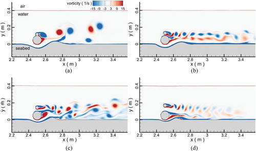
All the environmental variables in the simulation are the same as these in the physical experiment. In Figure 4, the evolution of scour hole and the vorticity flow field at three different times is displayed.

Figure 4. The evolution of the sandy bed and vorticity field around a piggyback pipe. (a) t = 2400 s, (b) t = 4800 s and (c) t = 18,000 s.

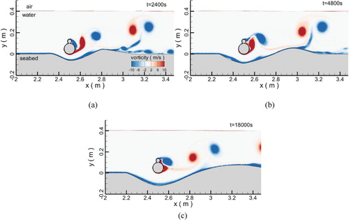
In this case, both the spacing-ratio and the gap-ratio are zero and the incoming flow velocity is 0.4 m/s. The results indicate that due to the constant influence of the flow, the scour hole becomes bigger and bigger. At the time of 2400 s, a small hole is scoured under the piggyback pipeline and the sediment is transported to the back of the pipeline. A sediment convex hull is formed behind the pipeline. With the development of scour hole, more and more sediment is transported to the rear of the pipeline. Finally, the scour reaches the equilibrium, and the scour hole is unchanged at the time of 18,000 s. The dynamic slope angles and the scour hole changes synchronously. Besides, the vortex sheds off the pipeline, and the shedding swirls affect the accumulated sediment behind the pipeline, which is lee-wake erosion.

Depending on the numerical simulation, it is also found that with the increase of scour hole, the velocity in the gap between the main pipe and sandy bed gradually decreases. When the velocity at the sandy bed is equal to the erosion-stopping velocity, the scour stops.

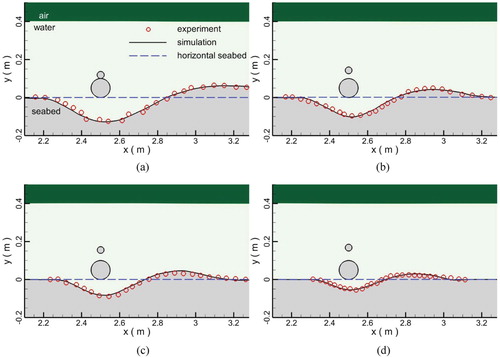
When the scour is in the equilibrium state, Figure 5 shows the comparison between the experimental data and simulation results about the predicted profiles of the scour hole. The velocity u₀ is 0.4 m/s and gap-ratio changes from 0 to 0.5. The numerical results are in good agreement with experimental data. Both the numerical results and experimental data indicate that the larger the gap ratio, the smaller the scour hole.

Figure 5. The scour hole comparison between experimental data and simulation results. (a) e₀ = 0.000, (b) e₀ = 0.250, (c) e₀ = 0.375 and (d) e₀ = 0.500.

When the incoming flow velocity is 0.24 m/s and the scour hole does not change, the shedding whirlpools behind the pipeline under different gap ratios are depicted in Figure 6. When the gap between small and main pipes does not exist, an integrated whole consisting of small and main pipes has a disturbing effect on the flow. And a large vortex is formed behind the pipeline in the wake region. With the increase of the gap-ratio, the mutual interaction between the shedding vortexes behind the small and main pipes becomes strong. When the gap ratio is 0.25, the vortexes are disordered. If the gap is significantly large, the intensity of the mutual interaction between the small and main pipes becomes weaker and weaker with the increase of the gap ratio. As seen in Figure 6(d), the vortexes behind the small and main pipes separate clearly. The size of the vortexes behind the pipeline also decreases. The smaller the shedding vortex is, the lower the pressure difference around the pipeline is, and the smaller the hydraulic gradient around the pipeline is. Furthermore, the mutual interaction of the shedding vortexes behind the small and main pipes has a significant effect on the development of the scour hole. Figure 6 clearly displays that the stronger the vortex intensity, the more serious the angle changes.

Figure 6. The vortex patterns around the pipelines with D = 0.1 m. (a) e₀ = 0.000, (b) e₀ = 0.125, (c) e₀ = 0.250 and (d) e₀ = 0.500.

4. Comparison and discussion

In this section, the change of dynamic slope angle is analysed in detail. The comparison between the test data and the simulation values for different conditions is also discussed.

4.1. Dynamic slope angle under the pipeline without spacing-ratio (e₀)

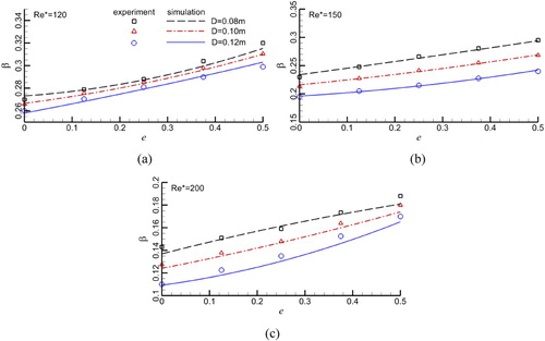
The relationship between grain Reynolds number (Re*) and dynamic slope angle (α and β) can be seen in Figures 7 and 8. The grain Reynolds number is defined as Re* = u·d₅₀/υ (where u is the incoming flow velocity, d₅₀ is the grain median diameter). In the figures, the lines and point symbols represent simulation curve and experimental data, respectively. The unit of slope angle is radian.

Figure 7. The change of upstream slope angle α at different gap ratios and pipe diameters.

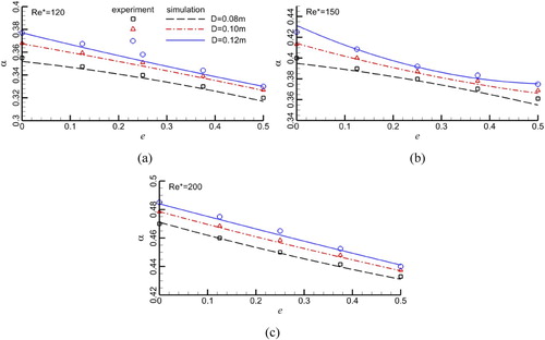
Figure 8. The change of downstream slope angle β at different gap ratios and pipe diameters.

As plotted in Figure 7, the gap-ratio has an important effect on the dynamic slope angle. With the increase of gap-ratio, the upstream slope angle α decreases. When the gap-ratio is zero, the angle α values change from 0.355 to 0.485. While, at a big gap-ratio (e.g. e = 0.50), the angle α values are within 0.320–0.440. With the increase of pipeline diameter and the grain Reynolds number, the dynamic slope angle α increases. When the grain Reynolds number is 150, the angle α values change from 0.33 to 0.377. When this number reaches 200, the α values rank within 0.44–0.47.

The change of downstream slope angle β is displayed in Figure 8. At the same pipe diameter and grain Reynolds number, the dynamic slope angle β increases with the increase of the gap ratio. At a big gap-ratio (e.g. e = 0.50), the values of angle β are ranks from 0.165 to 0.32. While, when the gap-ratio is zero, the values of angle β vary from 0.11 to 0.27. However, with the increase of grain Reynolds number, the dynamic slope angle β decreases. When this number is 120, the range of angle β is within 0.26-0.32. When the number is 150, the angle β values are from 0.11 to 0.188.

Depending on the comparison between the angle α and the angle β, the results show that at the same pipe diameter and gap-ratio (e), the angle α increases slightly with the increment of grain Reynolds number. However, the angle β changes reversely and the value decreases seriously. Besides, at the same grain Reynolds number, the angle α decreases slightly as the pipe diameter decreases; then, the angle β keeps increasing. It is found that the scouring influence factors have a more significant effect on the angle β than angle α. The smaller the gap-ratio is, the more obvious the trend is.

4.2. Dynamic slope angle under the pipeline with gap-ratio (e) and spacing-ratio (e₀)

In Figure 9, the dynamic slope angle has been plotted as a function of spacing-ratio (e₀) under different gap-ratios (e) in the grain Reynolds number of 120. Six spacing-ratios (e₀) are designed from 0.1 to 0.9. The gap ratios (e) are set to 0, 0.25 and 0.5. The incoming velocity (u₀) is 0.24 m/s.

Figure 9. The change of slope angle with different spacing-ratios. (a) upstream dynamic slope angle α and (b) downstream dynamic slope angle β.

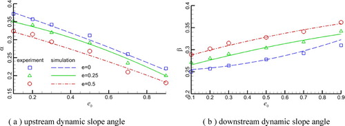
When both the gap-ratio (e) and the spacing-ratio (e₀) exist, the angle α decreases as the spacing-ratio (e₀) increases. The angle β has the opposite trend. At the same spacing-ratio, with the increase of gap-ratio, the angle α is decreasing and the angle β increases. For example, when the spacing-ratio is 0.5, the angle α is 0.312 at e = 0 and 0.268 at e = 0.5. However, the angle β is 0.278 at e = 0 and 0.328 at e = 0.5. With the increasing of spacing-ratio (e₀), the angle α changes from 0.18 to 0.372, and the angle β varies from 0.25 to 0.362.

The part experimental data and simulation values are displayed in Table 2. There is a satisfactory match between test data and simulation values. In conclusion, the results indicate that the ratios have an important effect on the dynamic slope angle.

Table 2 The part experimental values and simulation data for angle α and angle β.

					Angle α		Angle β
Runs	D(m)	e	u0	e0	Test	Simulation	Test	Simulation
01	0.08	0/0.25/0.5	0.24	0	0.355/0.340/0.320	0.352/0.338/0.317	0.270/0.288/0.321	0.273/0.286/0.315
02	0.08	0/0.25/0.5	0.30	0	0.401/0.382/0.361	0.395/0.379/0.355	0.231/0.266/0.295	0.234/0.263/0.294
03	0.08	0/0.25/0.5	0.40	0	0.471/0.451/0.433	0.471/0.449/0.431	0.143/0.159/0.188	0.137/0.162/0.181
04	0.10	0/0.25/0.5	0.24	0	0.368/0.351/0.327	0.367/0.348/0.327	0.266/0.286/0.310	0.267/0.284/0.311
05	0.10	0/0.25/0.5	0.30	0	0.414/0.387/0.369	0.414/0.385/0.366	0.214/0.242/0.269	0.216/0.239/0.269
06	0.10	0/0.25/0.5	0.40	0	0.479/0.459/0.438	0.479/0.457/0.437	0.128/0.148/0.180	0.124/0.147/0.174
07	0.12	0/0.25/0.5	0.24	0	0.377/0.358/0.332	0.377/0.352/0.331	0.260/0.281/0.299	0.258/0.279/0.303
08	0.12	0/0.25/0.5	0.30	0	0.425/0.392/0.375	0.431/0.389/0.375	0.195/0.215/0.241	0.196/0.213/0.242
09	0.12	0/0.25/0.5	0.40	0	0.485/0.465/0.440	0.484/0.462/0.441	0.110/0.135/0.170	0.109/0.129/0.165
10	0.12	0.25	0.24	0.3/0.5	0.320/0.291	0.315/0.294	0.291/0.304	0.288/0.306
11	0.12	0.25	0.30	0.3/0.5	0.355/0.340	0.351/0.338	0.280/0.290	0.276/0.286
12	0.12	0.25	0.40	0.3/0.5	0.415/0.400	0.412/0.396	0.200/0.225	0.191/0.215

4.3. Comparison and validation

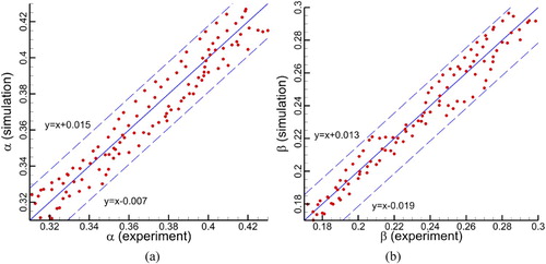
In order to verify the accuracy and reliability of the numerical model in predicting the dynamic slope angle, the simulation solutions have been compared with corresponding experimental data, as plotted in Figure 10. Figure 10(a) on the left belongs to the comparison of upstream dynamic slope angle α between simulation results and the experimental data. Correspondingly, Figure 10(b) on the right belongs to the comparison of downstream dynamic slope angle β. In the figure, the red points present the values of the simulation and the experiment in the same cases. For example, in Run 4, when the gap-ratio is 0.25, the experiment and simulation values of the upstream dynamic slope angle are 0.351 and 0.348, respectively. Therefore, the horizontal and vertical coordinates of the red point are 0.351 and 0.348, respectively (Figure 10(a)). When the experimental data are equal to the simulation data, the red points are on the blue line whose formula is y = x. The more the red points around the blue line, the better the comparison between the simulation results and the experimental results. The formula deviation ranges of α and β are from −0.007 to 0.015 and from −0.019 to 0.013, respectively.

Figure 10. Comparison between simulation values and data obtained from experimental measurement; (a) the upstream dynamic slope angle and (b) the downstream dynamic slope angle.

Besides, the convergence of the numerical results is also analysed to verify the numerical simulated model. The simulation adopts a dense mesh that has 542,585 elements with the finest grid spacing 0.02 mm next to the wall of the cylinder. To ensure resolution sufficiency of the computational mesh, another two meshes with 214,154 elements (medium mesh) and 25,489 elements (coarse mesh) are also employed. After the simulations, the numerical results are compared with the experimental data depending on the deviation method. The formula of deviation value is written as: Δ =|x_exp– x_num|/x_exp. x_exp and x_num are the experimental and numerical data of the dynamic slope angle at the same case, respectively. The deviation value of every case is calculated and the statistical results of all cases are shown in Figures 11 and 12. In the figure, the horizontal and vertical coordinates represent the deviation value and the frequency of the results, respectively. The formula of the frequency is presented as ω = n_e/N_t where n_e is the case number in different deviation intervals and N_t is the total number of the cases. For example, in Figure 11(a), when the deviation interval is from 2% to 2.5%, the case number during this interval is 31 and the total number of the cases is 198, so, the frequency is 15.66%. For the upstream dynamic slope angle, when the deviation interval is between 2.5% and 3% (Figure 11(a)), the frequency is the highest which is about 39.9%. For the downstream dynamic slope angle, the convergence is similar to that of the upstream dynamic slope angle (Figure 12(a)). The deviation interval of the highest frequency for the dense mesh is between 3% and 3.5%.

Figure 11. The deviation analysis between numerical and experimental data for convergence of the upstream dynamic slope angle.

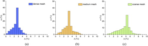
Figure 12. The deviation analysis between numerical and experimental data for convergence of the downstream dynamic slope angle.

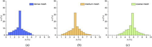
Depending on the comparison among subgraphs (a), (b) and (c) in Figures 11 and 12, it is found that with the number of the mesh grids decreasing, the type of mesh in the simulation model changes from the dense mesh to coarse mesh and the deviation interval of the highest frequency increases. The greater the deviation value is, the greater the difference between the numerical and experimental data is, and the worse the convergence of the numerical model is. Besides, even if the mesh grids are the same, the deviations of the experimental and numerical data are also different and the frequencies in the deviation range present a normal distribution in general. Correspondingly, in Figure 10, the comparison points between numerical and experimental data are also evenly distributed on both sides of the isocline y = x in the deviation range for both slope angles. There are three main reasons causing this deviation. Firstly, in the simulation model, the finite volume method (FVM) is adopted to discretise the governing equations. If the scale of mesh increases, the spatial distance of the center control points between adjacent grids also increases, which reduces the solution range density of the governing equations. If the important turbulence flow is not captured by the governing equations, the accuracy of numerical results may be affected. Besides, in the simulation, the moving-mesh technique is used for the change of seabed. When the scour happens, the mesh changes until the scour reaches equilibrium, which is also lead to the deviation of the result. So, in order to ensure the accuracy of the simulation, three different meshes are analysed and the accuracy of the simulation can be improved using the dense mesh. However, the deviation cannot be eliminated completely. Secondly, in some governing equations of the numerical model, such as continuous and momentum equations, only numerical solutions can be given instead of the analytical solutions, which introduces the approximate values. The deviation caused by the governing equations is an unsolvable problem for computational fluid dynamic method up to now. So, the deviation exists in every case. Thirdly, in the experiments, random and systematic errors cannot be avoided. For instance, the velocity is measured using the ADV which is located in the flow. Although the location of the equipment is selected specially to reduce the impact on flow, this equipment still can disturb the flow to some extent. When the fluid state changes, the fluid acceleration may cause slight change of the seabed. Besides, the errors may also occur in the measuring instruments and data collection system. So, in order to reduce the errors, many experiments are arranged and the deviation analysis is conducted for the simulation accuracy, as shown in Figures 10, 11 and 12. In addition, in the same case, the deviation frequencies of upstream and downstream slope angles are also different, as shown in Figures 11(a) and 12(a). Compared with the upstream slope angles, the downstream slope angles are smaller. Using the same measurement equipment, the random and systematic errors for downstream slope angles maybe more than that for upstream slope angles. So, the deviation frequencies of two type angles are different, but the highest frequency occurs in the similar deviation interval. It shows that the main factors affecting the upstream and downstream slope angles are the same.

Although some reasons cause the deviations of the numerical and experimental results, the deviations of all cases are within the allowable error of 10% and the dense mesh used in this model is sufficient. The computational capability of the present model is validated in predicting the scour around the piggyback pipeline.

5. Conclusions

This paper numerically and experimentally studies the dynamic slope angle of sandy bed underneath piggyback pipeline in steady flow. The influence of pipe diameter, spacing-ratio and gap-ratio on the angle has been analysed. The following main conclusions can be drawn on the basis of above discussion:

1. After analysis of the simulation results, it is apparently found that the gap-ratio has a significant influence on the intensity of the mutual interaction between the shedding vortexes behind the small and main pipes. When the gap between the small and main pipes does not exist, a large vortex is formed behind the pipeline in the wake region. With the increase of the gap, the mutual interaction causes the chaos of vortexes behind the pipelines. Once the gap is significantly large, there are a big vortex behind the main pipe and a small vortex behind the small pipe, respectively. The two vortexes do not interfere with each other.

2. The experimental and numerical results show that the local scour around the piggyback pipeline is affected by many factors, such as pipeline diameter, inflow velocity, gap-ratio and spacing ratio. The angle α increases slightly with the increment of the grain Reynolds number, but it decreases with the growth of the gap-ratio and spacing-ratio. However, the angle β changes reversely. Besides, the influence of environmental factors on angle β is more serious than angle α.

3. In order to verify the simulation model, the convergence of the numerical data is analysed depending on the deviation method. In general, there are three main reasons causing the deviation: the scale of the mesh, the numerical solutions of the governing equations, and the random and systematic errors of the experiment. In order to reduce the deviation, the mesh resolution of the numerical model is improved and many physical experiments are conducted. However, the deviations cannot be eliminated. In most cases, the deviations between the numerical and experimental data are between 2.5% and 3.5%, and in some cases, the maximum deviation reaches about 6.5%. Besides, the frequencies in the deviation range present a normal distribution and the comparison points between numerical and experimental data are also evenly distributed on both sides of the isocline y = x. Anyway, all deviations are within the allowable error of 10%. Therefore, the accuracy and reliability of the proposed simulation model in predicting the dynamic slope angles of seabed under piggyback pipeline are satisfied. The authors believe that the conclusions drawn from this work might provide the practical reference for the understanding of the scour around the piggyback pipeline, which could be helpful to the design of the submarine pipeline.

Disclosure statement

No potential conflict of interest was reported by the authors.

Additional information

Funding

This work was supported by the National Key Research and Development Program of China (grant number 2017YFC1404700), the Discipline Layout Project for Basic Research of Shenzhen Science and Technology Innovation Committee (grant number 20170418), the Guangdong Special Fund Program for Marine Economy Development (grant number GDME-2018E001), and the National Natural Science Foundation of China (grant number 41806010); Young Scientists Fund.

References

- Bayraktar D, Ahmad JL, Bjarke EC, Stefan F, David R. 2016. Experimental and numerical study of wave-induced backfilling beneath submarine pipelines. Coastal Eng. 118:63–75.
- Brørs B. 1999. Numerical modeling of flow and scour at pipelines. J Hydraul Eng. 125(5):511–523.
- Cheng X, Wang Y, Wang G. 2013. Influence of proximity of the seabed on hydrodynamic forces on a submarine piggyback pipeline under wave action. J Offshore Mech Arct Eng. 135(2):021701.
- Chiew YM. 1990. Mechanics of local scour around submarine pipelines. J Hydraul Eng. 116(4):515–529.
- Darwish M, Moukalled F. 2006. Convective Schemes for Capturing interfaces of free-surface flows on unstructured grids. Numer Heat Transf Fundam. 49(1):19–42.
- Dey S, Singh NP. 2007. Clear-water scour depth below underwater pipelines. J Hydro-Environ Res. 1(2):157–162.
- Engelund F, Fredsøe J. 1976. A sediment transport model for straight alluvial channels. Nord Hydrol. 7:293–306.
- Ferziger JH, Perić M. 2002. Solution of the Navier-Stokes equations. In: Computational methods for fluid dynamics. Berlin: Springer; p. 149–208.
- Fredsøe J, Deigaard R. 1992. Mechanics of coastal sediment transport. Singapore: World Scientific.
- García MH, Parker G. 1991. Entrainment of bed sediment into suspension. J Hydraul Eng. 117(4):414–435.
- Hirt CW, Nichols BD. 1981. Volume of fluid (VOF) method for the dynamics of free boundaries. J Comput Phys. 39:201–225.
- Huang CW, Zhan YZ, Lu JY. 2008. The formula of dynamic angle of repose for cohesive and non-cohesive uniform sediment. Guangdong Water Resour. Hydropower. 6:1–4.
- Issa RI. 1991. Solution of the implicitly discretised fluid flow equations by operator-splitting. J Comput Phys. 93(2):388–410.
- Jasak H, Tukovic Z. 2006. Automatic mesh motion for the unstructured finite volume method. Trans Famena. 30(2):1–20.
- Larsen BE, Fuhrman DR, Sumer BM. 2016. Simulation of wave-plus-current scour beneath submarine pipelines. J Waterw Port Coast Ocean Eng. 142(5):04016003.
- Leonard BP. 1991. The ULTIMATE conservative difference scheme applied to unsteady one-dimensional advection. Comput Methods Appl Mech Eng. 88(1):17–74.
- Liu X, Marcelo H. 2008. Three-dimensional numerical model with free water surface and mesh deformation for local sediment scour. J Waterw Port Coast Ocean Eng. 134(4):203–217.
- Rhie CM, Chow WL. 2012. Numerical study of the turbulent flow past an airfoil with trailing edge separation. AIAA J. 21(11):1525–1532.
- Sumer BM, Fredsøe J. 2002. The mechanics of scour in the marine environment. Singapore: World Scientific.
- Sumer BM, Jensen HR, Ye M, Oslash RF. 1988. Scour below pipelines in Waves. J Waterw Port Coast Ocean Eng. 116(3):599–614.
- Van Rijn L. 1984. Sediment transport. Part II: suspended load transport. J Hydraul Eng. 110(11):1613–1641.
- Yang FG, Liu XN, Yang KJ. 2009. Study on the angle of repose of nonuniform sediment. J Hydrodyn Ser B. 21(5):685–691.
- Yang H, Ni H, Zhu XH. 2007. An applicable replacement bundled pipeline structure for offshore marginal oilfield development. Shipbuild China. 48(B11):563–570.
- Yang LP, Shi B, Guo YK. 2012. Study on dynamic angle of repose for submarine pipeline with spoiler on sandy seabed. J Petroleum Explor Prod Technol. 2:229–236.
- Zang ZP, Gao FP. 2014. Steady current induced vibration of near-bed piggyback pipelines: configuration effects on VIV suppression. Appl Ocean Res. 46(2):62–69.
- Zang ZP, Gao FP, Cui JS. 2013. Physical modeling and swirling strength analysis of vortex shedding from near-bed piggyback pipelines. Appl Ocean Res. 40(3):50–59.
- Zhao EJ, Qu K, Mu L, Kraatz S, Shi B. 2019. Numerical study on the hydrodynamic characteristics of submarine pipelines under the impact of real-world Tsunami-like waves. Water (Basel). 11(2):221.
- Zhao EJ, Shi B, Qu K, Dong WB, Zhang J. 2018. Experimental and numerical Investigation of local scour around submarine piggyback pipeline under steady currents. J Ocean Univ China. 17(2):244–256.
- Zhao EJ, Shi B, Zhang J, Cao K. 2015. Numerical simulation of mass ratio’s effect on vortex-induced vibration of suspended submarine pipeline. Proceedings of 2015 International Conference on Computer Information Systems and Industrial Applications, Bangkok, Thailand, 902–904.
- Zhao M, Cheng L. 2008. Numerical modeling of local scour below a piggyback pipeline in currents. J Hydraul Eng. 134(10):1452–1463.
- Zhao M, Vaidya S, Zhang Q, Cheng L. 2015. Local scour around two pipelines in tandem in steady current. Coastal Eng. 98:1–15.
- Zhou YC, Xu BH, Yu AB, Zulli P. 2002. An experimental and numerical study of the angle of repose of coarse spheres. Powder Technol. 125(1):45–54.