Numerical simulation of the two-degree-of-freedom vortex induced vibration of a circular cylinder at Reynolds number of O(10⁴∼10⁵)

Abstract

Vortex induced vibration (VIV) is of practical interest since it can result in the fatigue damage of structures, so has been a highly researched topic during the past few decades. The present study employs the unsteady Reynolds-Averaged-Navier–Stokes (URANS) equations combined with the shear-stress transport (SST) k-ω turbulence model to carry out the numerical simulation of the two-degree-of-freedom (2DOF) VIV at Reynolds number of O(10⁴∼10⁵). The present numerical method is validated through the comparison of the numerically and experimentally obtained response amplitude, lock-in frequency and hydrodynamic force, and the obtained vortex shedding modes are demonstrated. Based on the numerical model, this study parametrically investigates the effect of the Reynolds number, mass-damping ratio on the 2DOF VIV. The results indicate that the changes of the Reynolds number in the range of 10⁴∼10⁵ seem to have little effect on the VIV, and the maximum non-dimensional amplitude of the cross-flow (CF) VIV keeps close to 1.5. The in-line (IL) VIV is more sensitive to the Reynolds number than CF VIV. Additionally, with the increase of the mass-damping ratio, the peak of the CF non-dimensional amplitude in 2DOF VIV decreases, and its difference with that in 1DOF VIV decreases.

1. Introduction

Vortex induced vibration (VIV) of bluff structures in fluid flow is a very common phenomenon in many engineering applications, such as risers in offshore engineering, bridge piers, etc. If the vortex shedding frequency is close to the natural frequency of the structures, the vortex shedding would be synchronised with the vibration of the structures, i.e. lock-in. When the lock-in occurs, the VIV amplitude can be significantly amplified, which may expedite the fatigue failure of these structures. Therefore, many researches have been focused on the VIV characteristics and suppression during the past few decades, as reviewed by Sarpkaya (1979, 2004), Parkinson (1989), Williamson (1996), Williamson and Govardhan (2008), and Wu et al. (2012).

VIV has the self-excited and self-limited features, and it is widely accepted that the associated amplitude and lock-in range can be affected by several non-dimensional parameters: the mass ratio (m*) defined as m/m_d, where m and m_d represent the mass of the cylinder and its displaced fluid, respectively; the structural damping ratio (ζ) defined as δ/2π (Rahmanian et al. 2012), where δ is the logarithmic decrement; the reduced velocity (U_r) defined as U/(f_ND), where U is the fluid velocity, f_N is the natural frequency of the cylinder in still fluid, D is the diameter of the cylinder; the Reynolds number (Re) defined as UD/v, where v is the kinematic viscosity of the fluid.

Feng (1968) carried out cross-flow (CF) VIV experiment in a wind tunnel using a cylinder with mass ratio of 248. It was found that there are two branches for the profile of non-dimensional amplitude. Khalak and Williamson (1996) presented the experimental results of a cylinder with low mass ratio of 2.4 in water. The interesting finding is that another branch, named upper branch, is observed with the maximum non-dimensional amplitude up to about 1.0, obviously larger than that in Feng (1968). Following this, Khalak and Williamson (1999) proposed a modified Griffin plot in terms of mass-damping ratio defined as α = (m*+C_A)ζ, showing reasonable trend of the maximum non-dimensional amplitude, where C_A is the added mass coefficient. Jauvtis and Williamson (2004) found that when adding the vibration in the in-line (IL) direction, i.e. two-degree-of-freedom (2DOF) VIV, the non-dimensional amplitude in the upper branch would be approximately amplified to 1.5 for small mass ratio, so this branch is called super-upper branch. With mass ratio increasing, the non-dimensional amplitude would decrease to about 1.0 at mass ratio of about 6.0. Subsequently, Stappenbelt et al. (2007), Sanchis et al. (2008), Blevins and Coughran (2009), Gonçalves et al. (2012) and Kang et al. (2016) conducted the 2DOF VIV experiments to investigate the effect of the mass ratio, structural damping and aspect ratio on the VIV response. In these studies, small mass-damping ratios were applied. The Reynolds number is a fundamental parameter for the definition of vortex shedding, thus affecting the VIV response (Belloli et al. 2015). Ding et al. (2004), Raghavan and Bernitsas (2011) and Narendran et al. (2015) carried out a series of one-degree-of-freedom (1DOF) VIV experiment with Reynolds number up to the order of 10⁵. As for the 2DOF VIV experiment at high Reynolds number, the publications can be rarely found.

With the development of the numerical methods and computational resources, the numerical simulation of the VIV has been widely investigated during the past decades. The early studies mainly focused on the 1DOF VIV simulation, see Zhou et al. (1999), Guilmineau and Queutey (2004), Pan et al. (2007), Wanderley et al. (2008) and Li et al. (2011). Recent years the 2DOF VIV simulation has been paid much attention to, and the super-upper branch was reproduced (Zhao et al. 2012; Gsell et al. 2016; Zhang et al. 2017; Pastrana et al. 2018). Wang et al. (2017) investigated the 2DOF VIV under different IL to CF natural frequency ratios, and found that the peak amplitude shifts to higher reduced velocity when the frequency ratio increases from 1 to 2. Xu et al. (2014) and Song et al. (2017) carried out the simulation for the VIV suppression by attaching different devices on the cylinder surface. Huang et al. (2008) investigated the effect of the Reynolds number on the cylinder’s VIV based on the numerical simulation.

Above mentioned numerical simulation is limited to the Reynolds numbers at the order of 10³. Nguyen and Nguyen (2016) indicated that the resolution of the flow features would become challenging for numerical simulation of VIV at high Reynolds number in the range of 10⁴–10⁶, at which the flow exhibits transitions to turbulent or fully turbulent behaviours. Therefore, some researchers attempted to apply different turbulence models to simulate the flow past a circular cylinder at high Reynolds number. But most of them focused on the stationary cylinder in the flow. As for the VIV, only few works were reported. Ong et al. (2009) numerically simulated the flow around a stationary cylinder at Reynolds number up to 10⁶ using the k-ε turbulence model. Prsic et al. (2014) investigated the flow around a smooth circular cylinder in uniform current at Reynolds number of 10⁴ based on the large eddy simulation (LES). Stringer et al. (2014) employed two solvers: OpenFOAM and CFX, both with shear-stress transport (SST) k-ω turbulence model, to simulate the flow around a stationary cylinder at a wide range of Reynolds numbers. The results indicated that the lift coefficient obtained from OpenFOAM falls in the scatter of the experimental data at the Reynolds number smaller than 10⁴, but when the Reynolds number ranges from 10⁵ to 10⁶, the CFX performs more reasonably with an error less than 15% from the experimental data. Ye and Wan (2017) carried out further works using OpenFOAM with SST k-ω turbulence model, and validated the conclusions in Stringer et al. (2014). Yeon et al. (2016) conducted large-eddy simulation of turbulent flow past a stationary cylinder at subcritical Reynolds numbers, and the results showed good agreement with experimental data. Nguyen and Nguyen (2016) utilised a hybrid turbulence model based on the URANS and LES to carry out the simulation of 2DOF VIV with Reynolds number ranging from 3 × 10³ to 3 × 10⁴, and the predicted results were similar with the experimental data in Jauvtis and Williamson (2004).

For better understanding of the 2DOF VIV, this study numerically investigates the VIV characteristics of a circular cylinder at Reynolds number in the range from 10⁴ to 10⁵ by using the URANS equations. The k-ε and SST k-ω turbulence models are assessed, and it is found that the latter may be more preferable for the VIV simulation. The mesh independence of the computational domain is tested by the convergent analysis. Then the numerical model is validated against the experimental results in Jauvtis and Williamson (2004). Based on this numerical model, the present study investigates the effect of the Reynolds number, mass ratio and damping ratio on the 2DOF VIV, and some useful conclusions are obtained.

2. Methodology

2.1. Numerical formulations

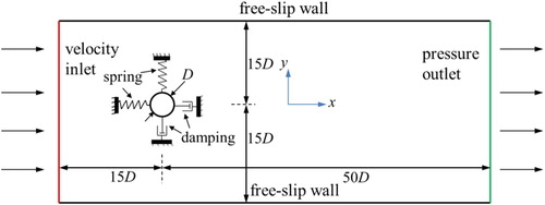
In the present study, the simulation of flow past an elastically supported cylinder is carried out in the two-dimensional (2D) framework, see Figure 1. The flow can be described by the URANS equations as follows: (1) $\frac{\mathrm{\partial }{U}_i}{\mathrm{\partial }{x}_i}=0$(1) (2) $\frac{\mathrm{\partial }}{\mathrm{\partial }t}\left(\rho U_i\right)+\frac{\mathrm{\partial }}{\mathrm{\partial }{x}_j}\left(\rho U_i{U}_j\right)=-\frac{\mathrm{\partial }p}{\mathrm{\partial }{x}_i}+\frac{\mathrm{\partial }}{\mathrm{\partial }{x}_j}\left(2\mu S_{ij}-\rho \overline{{u^{\mathrm{\prime }}}_i{u^{\mathrm{\prime }}}_j}\right)$(2) where U_i and x_i represent the instantaneous velocity and Cartesian coordinate in i direction, U_j and x_j represent the instantaneous velocity and Cartesian coordinate in j direction, p is the pressure, t is time, ρ is the fluid density, μ is molecular viscosity, S_ij is the mean strain tensor, written as: (3) $S_{ij}=\frac{1}{2}\left(\frac{\mathrm{\partial }{U}_i}{\mathrm{\partial }{x}_j}+\frac{\mathrm{\partial }{U}_j}{\mathrm{\partial }{x}_i}\right)$(3) The $-\overline{{u^{\mathrm{\prime }}}_i{u^{\mathrm{\prime }}}_j}$ denotes the Reynolds stress component, and can be expressed using the Boussinesq hypothesis: (4) $-\overline{{u^{\mathrm{\prime }}}_i{u^{\mathrm{\prime }}}_j}=2{\upsilon }_t{S}_{ij}-\frac{2}{3}{\delta }_{ij}k$(4) where υ_t is turbulent kinematic viscosity, k is the turbulent energy, δ_ij is the Kronecker delta.

Figure 1. Computational domain of the flow past an elastically supported cylinder.

The Reynolds stress can to some extent represent the effect of turbulence, but meanwhile introduces two variables: υ_t and k. Therefore, a turbulence model should be introduced to close Equation (2). As mentioned in the introduction, the k-ε and SST k-ω turbulence models are often employed in the simulation of flow past a cylinder, and predict reasonable results. This study would compare the two turbulence models in Section 2.2, and select one to conduct the 2DOF VIV analysis of a circular cylinder.

The response of an elastically supported cylinder in x and y directions can be governed by: (5) ${\ddot{x}}_c+2\zeta {\omega }_0{\dot{x}}_c+{\omega }_0^2{x}_c=\frac{F_x\left(t\right)}{m}$(5) (6) ${\ddot{y}}_c+2\zeta {\omega }_0{\dot{y}}_c+{\omega }_0^2{y}_c=\frac{F_y\left(t\right)}{m}$(6) Where x_c and y_c represent the displacement of the cylinder along x and y directions, respectively, m is the mass of the cylinder, ω₀ = 2πf_n, ζ and f_n is the structural damping ratio and natural frequency of the system in vacuum, F_x and F_y are the hydrodynamic forces in x and y directions, respectively. The current is along x direction, so x and y correspond to the IL and CF directions, respectively. According to Jauvtis and Williamson (2004), the IL and CF displacement can be approximately expressed as: (7) $x_c=A_x\sin \left(2\omega t+\theta \right),y_c=A_y\sin \left(\omega t\right)$(7) where A_x and A_y are the response amplitude in IL and CF directions, respectively, ω = 2πf, f is the CF VIV frequency, θ is the phase difference between IL and CF VIV. The IL and CF non-dimensional amplitude is defined as $A_x^{\ast }=A_x/D$ and $A_y^{\ast }=A_y/D$, respectively.

The commercial software, Fluent14.5 is applied to carry out the simulation of the fluid and cylinder interaction in this study. At each time step, the pressure around the cylinder surface is integrated to calculate the hydrodynamic force, which is substituted into Equations (5) and (6) to determine the cylinder motion using the Newmark-β method. The obtained cylinder motion is then input to the solver through the user-defined functions (UDFs) for the next step of the calculation. The mesh deformation induced by cylinder motion can be well modelled by the dynamic mesh method (Zhu and Yao 2015). This study conducts these analyses in windows 7 platform with Intel(R) Xeon(R) CPU E3-1226 and 8 GB RAM.

2.2. Mesh resolution test

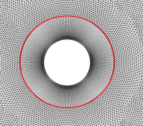
The computational domain shown in Figure 1 is discretized with triangular and four-point cells. Figure 2 demonstrates part of the mesh near the cylinder. Four-point cells are applied in the domain circled by the red line, which would move with the cylinder to increase the accuracy in simulating the flow around the cylinder. The triangular cells are used in the rest computational domain. It is widely accepted that the mesh density and the first layer height adjacent the cylinder surface can affect the simulation accuracy (Zhu and Yao 2015). Therefore, this section would conduct the mesh resolution test using the elastically supported cylinder in Jauvtis and Williamson (2004), which also would be employed in Section 3 for validation. The cylinder has a natural frequency of 0.4 Hz in still water with m* = 2.6. The surface of the cylinder is divided by n_c nodes, and has an adjacent layer with height of h. By changing n_c, the mesh density can be controlled. As for the h, different values were used in the published researches, see Guilmineau and Queutey (2004) and Rahmanian et al. (2012).

Figure 2. Mesh around the cylinder surface.

Firstly, the sensitivity of the VIV response to h is investigated under U_r = 6 based on the k-ε and SST k-ω turbulence models. It should be mentioned that the enhanced wall treatment is used in the k-ε turbulence model. In these analyses, the n_c is set to 200, which is used in Wanderley et al. (2008). Figure 3 shows the results obtained in the 1DOF VIV analyses. It can be seen that with h decreasing the $A_y^{\ast }$ and frequency ratio (f/f_N) exhibit increasing and decreasing trends, respectively, and tend to constant values at about h = 0.003D. 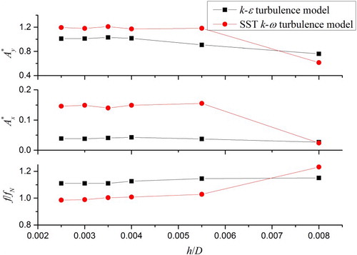Additionally, the k-ε turbulence model predicts higher $A_y^{\ast }$, but lower f/f_N than SST k-ω turbulence model. According to Figure 4, the convergent speed of the 2DOF VIV data seems to be faster than that of 1DOF VIV data. Compared with the k-ε turbulence model, the SST k-ω turbulence model predicts larger $A_y^{\ast }$ and $A_x^{\ast }$, but smaller f/f_N. The 2DOF VIV results of the experiment are $A_y^{\ast }$ = 1.16, $A_x^{\ast }$ = 0.19 and f/f_N = 0.96, so the percentage errors of these parameters for the k-ε turbulence model are 13.3%, 78.9% and 15.6%, respectively, and are 2.4%, 20.2% and 2.5% for the SST k-ω turbulence model. Overall, the SST k-ω turbulence model may be more suitable for the 2DOF VIV analysis. Additionally, there are some publications indicating that the k-ε turbulence model is not sophisticated with the simulation of the flow past a cylinder at subcritical Reynolds number (Franke et al. 1989, Tutar and Holdø 2001). The reason may be that the assumption of fully turbulent flow is applied in the k-ε turbulence model (Launder and Spalding 1972). Therefore, this study would employ the SST k-ω turbulence model to conduct the 2DOF VIV analysis, and the h is simply set to be 0.003D, which approximately corresponds to y+ near 1.0.

Figure 3. 1DOF VIV response under different h and turbulence models.

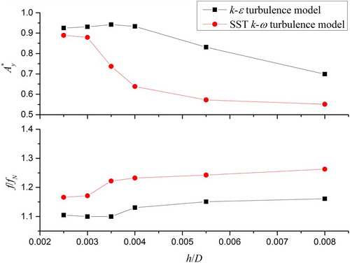
Figure 4. 2DOF VIV response under different h and turbulence models.

In order to investigate the effect of the mesh density on the VIV response, this study selects four cases with different n_c, and in detail investigates the related VIV response, see Table 1, where the C_D is the mean drag coefficient, the C_x,rms and C_y,rms are the root mean square (RMS) of the force coefficient in x direction (C_x) and in y direction (C_y), respectively. Taking the C_x as an example, the force coefficient is defined as C_x = 2F_x/(ρU²DL), where L is the cylinder length. The percentage difference of the VIV parameters for the previous cases is listed in the bracket. Compared with the meshes M3 and M4, the meshes M1 and M2 give smaller C_y,rms, but larger $A_y^{\ast }$. However, as for C_x,rms and $A_x^{\ast }$, the situation is opposite. The reason may be that the first two meshes predict the CF frequencies closer to f_N. With the increase of the mesh density, the percentage differences of all VIV parameters almost have a decreasing trend, and reach to very small values. So it can be considered that the results are convergent. When changing the mesh density from M3 to M4, the maximum percentage difference for the parameters is just 0.9%, but the computational time is changed from 54.2 to 63.6 CPU hours. Obviously, the accuracy of the predicted results is just improved less than 0.9% with the sacrifice of more 17.3% computational time. Therefore, M3 can provide an acceptable compromise between computational efficiency and accuracy.

Table 1. VIV parameters under different mesh densities.

Mesh	Cells	nc	f/fN	CD	Cx,rms	Cy,rms	$A_x^{\ast }$	$A_y^{\ast }$
M1	27982	120	1.023	2.87	1.24	1.59	0.142	1.241
M2	34238	160	0.961 (6.1%)	2.52 (12.2%)	1.19 (4.0%)	1.65 (5.0%)	0.148 (4.1%)	1.179 (5.0%)
M3	42761	200	0.933 (2.9%)	2.42 (4.0%)	1.14 (4.2%)	1.71 (2.4%)	0.151 (1.9%)	1.136 (3.6%)
M4	51407	240	0.928 (0.5%)	2.43 (0.4%)	1.13 (0.9%)	1.72 (0.6%)	0.152 (0.7%)	1.127 (0.8%)

3. Validation

Jauvtis and Williamson (2004) in detail reported the 2DOF VIV experiment of a cylinder. Based on this experimental model, this study carries out a series of VIV analysis under different U_r in the range from 3 to 13.5. The diameter of the cylinder is 0.0381 m. Correspondingly, the Reynolds number ranges from 1742 to 7839. In these analyses, the flow velocities gradually increase to the specific values. Figure 5 demonstrates the CF and IL VIV response normalised by D, and the corresponding figure-of-eight trajectories at Ur = 3.0, 8.0 and 10.0. It can be seen that the VIV is approximately harmonic. For Ur = 3.0, 8.0 and 10.0, the CF frequencies are 0.54, 1.02 and 1.26 Hz, respectively, and the IL frequencies are, in turn, equal to 1.08, 2.04 and 2.56 Hz. The IL frequencies are about 2 times CF frequencies. Therefore, the IL and CF displacement can be approximately expressed using Equation (7). The motion orbit is a regular Figure 8 at Ur = 3.0, while for Ur = 8.0 and 10.0, the motion are very flat due to the small IL motion, especially for Ur = 8.0, exhibiting a crescent shape. The motion direction marked by the red arrow is determined by the θ (Jauvtis and Williamson 2004).

Figure 5. VIV response and trajectories obtained from numerical simulation: (a) and (d) U_r = 3.0; (b) and (e) U_r = 8.0; (c) and (f) U_r = 10.0.

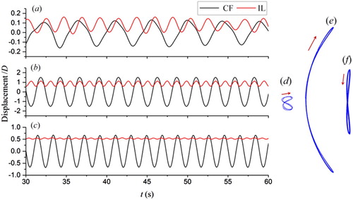
Figure 6 plots the VIV non-dimensional amplitude, f/f_N and θ as a function of Ur. This study takes the average values of the peaks in the steady response as the VIV amplitude. It can be seen that the super-upper branch of the CF VIV is reasonably captured, and shows well agreement with the experimental data. At the lower branch, the numerical simulation also predicts satisfying results, but overestimates the results at the initial branch. The IL VIV is overestimated at U_r in the range of 4.0–5.0. However, at the U_r corresponding to the super-upper and lower branch of CF VIV, the numerically obtained IL VIV is smaller than the experimental data. It should be noted that another peak of IL VIV near U_r = 3.0 is well captured. According to the f/f_N curve, the predicted frequencies of CF VIV have similar trend with the experimental data, that is, with the U_r increasing, the response frequency initially follows the curve related with Strouhal (St) frequency, and then starts to deviate from the curve at about U_r = 5, keeping slightly increase from 0.85f_N to 1.38f_N. The St frequency is the vortex shedding frequency when the flow passes a fixed cylinder (Pan et al. 2007). When the U_r increases to 13.5, there are two frequencies: one is about 1.38f_N, another is close to St frequency. Two response frequencies at large U_r are also observed by (Blevins and Coughran 2009). Under given CF and IL VIV amplitudes, the θ can determine the trajectory shape of VIV, see Jauvtis and Williamson (2004) for detail. As for the trajectories at U_r= 3.0, 8.0 and 10.0 shown in Figure 5, the predicted values of θ are about 190, 325 and 315 deg, respectively. Figure 6 illustrates that the θ is slightly overestimated at U_r smaller than 8.0, but shows good agreement with the experimental data at U_r larger than 8.0.

Figure 6. Comparison of the VIV Response between present study and experimental data.

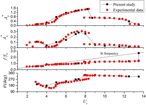
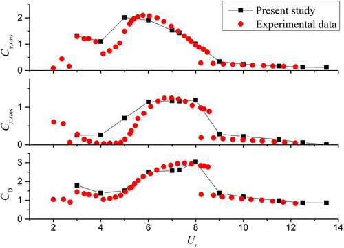
Figure 7 presents the vorticity contours at the position with Y = 0 and the time histories of force coefficients for Ur = 3.0, 8.0 and 10.0. The X and Y represent x_c/D and y_c/D, respectively. The red arrow denotes upward motion. Figure 7(a–c) demonstrate the 2S, 2T and 2P wake modes, respectively. These modes are reported in Jauvtis and Williamson (2004), especially for 2 T mode, which is associated with the super-upper branch. The IL force coefficients seems to be more regular than the CF force coefficient, see Figure 7(d–f). There are two components at U_r = 8.0 with frequencies equal to f and 3 times f. The CF force coefficients marked by the blue points in Figure 7(d–f) correspond to Figure 7(a–c). By analysing the position and moving direction of the cylinder, and the associated force coefficient curve in Figure 7, it can be noted that when the cylinder moves towards positive direction from the position of Y = 0, the CF force coefficient increases approximately from C_y = 0 at U_r = 3.0 and 8.0, but decreases approximately from C_y = 0 at U_r = 10.0. So the CF force coefficient is synchronised with the CF displacement at U_r = 3.0 and 8.0, but is opposite with the CF displacement at U_r = 10.0. Therefore, it can be concluded that the phase angles between CF displacement and CF force coefficient are about 0° at U_r = 3.0 and 8.0, but is about 180° at U_r = 10.0. This conclusion is the same with that in Jauvtis and Williamson (2004). Figure 8 compares the C_x,rms, C_y,rms, and C_D obtained from the numerical simulation and experiment, respectively. It can be seen that the as well as the non-dimensional amplitudes in Figure 6, the predicted C_y,rms and C_x,rms are obviously overestimated at U_r in the range of 4.0–5.0. However, the numerical simulation predicts reasonable results at U_r>6.0. As for the C_D, the predicted data is very close to the experimental data.

Figure 7. Vorticity contour and the time histories of the force coefficients: (a) and (d) U_r = 3.0; (b) and (e) U_r = 8.0; (c) and (f) U_r = 10.0. (a), (b) and (c) are the vorticity contours with the cylinder at Y = 0.

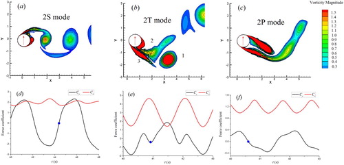
Figure 8. Comparison of force coefficient between present study and experimental data.

4. Parametric analysis

4.1. Effect of the Reynolds number

In the present study, five cases with m* = 2.8 and ζ = 0.6% are applied to investigate the effect of Reynolds number on the 2DOF VIV. Table 2 summarises the study parameters. The Reynolds numbers are in the range provided by the numbers in the square brackets, about at the order of 10⁴∼10⁵. The first four cases have the same natural frequency, and the increase of the Reynolds number is achieved by the increase of D. The case A5 increases the spring stiffness on the basis of case A4 to get larger natural frequency, so corresponds to larger Reynolds number than case A4 under given U_r. Figure 9 demonstrates non-dimensional amplitude under different Reynolds numbers. It can be seen that the maximum $A_y^{\ast }$ is close to 1.5. As the Reynolds number increases from case A1 to case A4, the maximum $A_y^{\ast }$ and $A_x^{\ast }$ both have a very slightly decreasing trend. However, when changing cases from A4 to A5, the maximum $A_y^{\ast }$ has a small increase. Additionally, the comparison of CF and IL VIV indicates that the IL VIV seems to be more sensitive to the Reynolds number. Overall, the changes in Reynolds number in the range of 10⁴∼10⁵ seem to have little effect on the numerically obtained results of 2DOF VIV, especially for CF VIV. This conclusion can also be obtained by the comparison of the experimental data from Jauvtis and Williamson (2004) and Stappenbelt et al. (2007) with the Reynolds number at the order of 10³ and 10⁴, respectively.

Figure 9. Non-dimensional amplitude as a function of U_r under different Reynolds numbers.

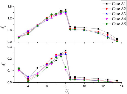
Table 2. Parameters of the elastically supported cylinder with different Reynolds numbers.

Case	A1	A2	A3	A4	A5
D (m)	0.055	0.070	0.090	0.100	0.100
fN (Hz)	0.982	0.982	0.982	0.982	1.664
m*	2.8	2.8	2.8	2.8	2.8
Re (×10^4)	[0.89, 3.90]	[1.44, 6.24]	[2.38, 10.3]	[2.94, 12.7]	[4.98, 22.4]

4.2. Effect of the mass ratio and damping ratio

It is widely known that the VIV of circular cylinders can be significantly affected by the mass ratio and damping ratio (Raghavan and Bernitsas 2011). However, the influence of the mass ratio and damping ratio on the 2DOF VIV is scarcely investigated by using numerical simulation, especially at high Reynolds number. Therefore, this study conducts the related analysis by using a circular cylinder with diameter of 0.055 m. The Reynolds number is on the order of 10⁴. Table 3 presents the applied four cases with varying mass ratio, and three cases with varying damping ratio.

Table 3. Values of mass and damping ratio.

Case	B1	B2	B3	B4	C1	C2	C3
m*	2.8	3.8	4.8	6.8	2.8	2.8	2.8
ζ (%)	0.6	0.6	0.6	0.6	0.6	6	20

As the mass ratio increases, the super-upper and lower branches of CF VIV would decrease, see Figure 10. As for the initial branch, it seems to be independent of the mass ratio. For the first two cases, the position of maximum $A_y^{\ast }$ is about at U_r = 8.0, while increasing the mass ratio to 4.8, the position decreases to about U_r = 6.0, which approximately corresponds to the position of $A_y^{\ast }$ profile peak of 1DOF VIV. With the increase of the mass ratio, the lock-in range decreases. Compared with CF VIV, the IL VIV is more sensitive to the mass ratio. The peak of $A_x^{\ast }$ profile for U_r larger than 4.0 would be obviously mitigated by the increasing mass ratio, and even decreases to a value smaller than the peak near U_r = 3.0. It can be seen that the peak near U_r = 3.0 tend to a constant value about equal to 0.075 with the increase of mass ratio. Figure 11 demonstrates the maximum non-dimensional amplitude as a function of mass ratio, in which the experiment (Stappenbelt et al. 2007) applied a circular cylinder with a diameter of 0.0554 m. It can be seen that the present results show reasonable agreement with the experiment.

Figure 10. Non-dimensional amplitude as a function of U_r under different m*.

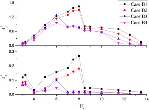
Figure 11. Maximum non-dimensional amplitude with increasing mass ratio.

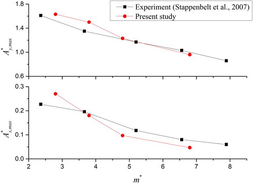
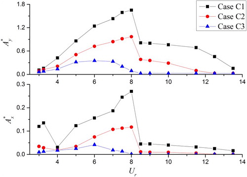
Figure 12 demonstrates that the increase of the damping ratio can significantly decreases the non-dimensional amplitude and the lock-in range. As for the CF VIV, the VIV amplitude at U_r larger than 10.0 seems to be more sensitive to the damping ratio than that at U_r smaller than 10.0. This is similar with the conclusion in Gsell et al. (2016). Different from the mass ratio, the damping ratio can extensively affect the peak of the $A_x^{\ast }$ profile near U_r = 3.0. Overall, the effect of the damping ratio on the $A_y^{\ast }$ and $A_x^{\ast }$ seems to be larger than the mass ratio.

Figure 12. Non-dimensional amplitude as a function of U_r under different ζ.

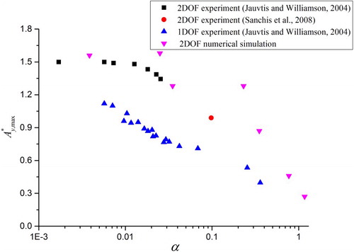
Jauvtis and Williamson (2004) demonstrated the peaks ($A_{y,max}^{\ast }$) of 1DOF and 2DOF VIV non-dimensional amplitude profiles in the Griffin plot in terms of α. But the data of 2DOF VIV is just under small α. Sanchis et al. (2008) added an experimental data in this Griffin plot for 2DOF VIV at α = 0.094. Overall, the variation trend of the $A_{y,max}^{\ast }$ with α for 2DOF VIV is not clear. In this study, except for the cases in Table 3, the analyses of three other cases are conducted: (1) m* = 2.85, ζ = 0.1%; (2) m* = 4.85, ζ = 0.6%; (3) m* = 4.85, ζ = 20%, and the obtained data are added to the Griffin plot, see Figure 13. Although the numerically obtained data is scattered, the trend is similar with the experimental data of 2DOF VIV. Additionally, it can be seen that the difference of $A_{y,max}^{\ast }$ between 2DOF and 1DOF VIV decreases with increasing α. The reason may be that the increase of α corresponds to the increase of the m* and ζ, and with the increase of m* and ζ, the IL VIV obviously decreases, see Figures 10 and 12, so the effect of the IL VIV on the CF VIV would decrease, leading to that the CF amplitude of 2DOF VIV tends to that of the 1DOF VIV.

Figure 13. The ‘Griffin’ plot of 1DOF and 2DOF VIV.

5. Conclusions

The present study aims to investigate the VIV characteristics of elastically supported cylinder at Reynolds number of O(10⁴∼10⁵) by using URANS equations. Firstly, the comparison of the k-ε and SST k-ω turbulence models and the mesh resolution test are conducted to select the most suitable turbulence model and mesh density. In the finial numerical model, the SST k-ω turbulence model is applied, and the mesh has 200 nodes at the cylinder surface with the height of adjacent layer equal to 0.003D. Through the comparison with the experiment in terms of response amplitude, frequency and hydrodynamic coefficient, the numerical model is in detail validated. Based on the parametric investigations conducted with this numerical model, some conclusions are obtained as follows:

1. The predicted maximum CF and IL VIV non-dimensional amplitudes are close to 1.5 and 0.25, respectively. For the CF VIV, the non-dimensional amplitude is similar with the published results at the Reynolds number of 10³. With the Reynolds number increasing the maximum non-dimensional amplitude seems to slightly decrease. Additionally, the IL VIV seems to be more sensitive to the Reynolds number than CF VIV.

2. As the mass ratio and damping ratio increase, the amplitudes and lock-in ranges of the CF and IL VIV decrease as expected. The peak of the IL VIV non-dimensional amplitude profile near U_r = 3.0 tends to about 0.075 with the increase of mass ratio, but tends to zero with the increase of damping ratio.

3. The predicted maximum CF VIV non-dimensional amplitude shows reasonable trend in the ‘Griffin’ plot in terms of α. The difference between 2DOF and 1DOF VIV in this plot decreases with increasing α.

Overall, the URANS equation combined with the SST k-ω turbulence model can well capture the 2DOF VIV features, and can reflect the effect of the mass ratio and damping ratio on the 2DOF VIV. However, the rationality of the predicted peak of the non-dimensional amplitude profile and ‘Griffin’ plot should be further verified based on the 2DOF VIV experiment at Reynolds number of O(10⁴∼10⁵).

Disclosure statement

No potential conflict of interest was reported by the authors.

Additional information

Funding

The authors would like to thank the financial support by the National Natural Science Foundation of China [grant number 51709135] and the Natural Science Foundation of Jiangsu Province [grant number BK20160557].