An improved control-limit-based principal component analysis method for condition monitoring of marine turbine generators

Abstract

The safe operation of marine turbine generators is a crucial concern in industries and academics. It is always important to monitor the health status of marine turbine generators. The lubricant oil usually carries abundant information on the turbine operation conditions. Various oil parameters of the turbines have been used in the existing monitoring systems. However, many of them conflict with each other by contrary detection results. Hence, it should eliminate the redundant oil parameters for efficient condition monitoring. Although many research studies addressed the redundant feature reduction issue using principal component analysis (PCA), PCA is designed for features with a linear relationship, which is not the case in marine turbine generator monitoring. This paper proposes a new nonlinear analysis method, the improved control-limit based PCA, to extract distinct failure indicators from the oil parameters of marine turbine generators. The contribution of this method is that the Hotelling statistic and Q statistic are combined to calculate a fixed control limit for PCA. The ability of the improved PCA to dealing with nonlinearity has been significantly enhanced by the proposed method. Experimental validation demonstrates that the extracted failure indicator using the proposed method is more effective than existing monitoring indexes with respect to fault detection accuracy.

1. Introduction

The widespread deployment of turbine generators raises increasing requirement on a high-standard condition monitoring strategy to guarantee the safe operation of the turbines (Katnam et al. 2015). This is particularly true for marine power plants, where the condition monitoring and fault diagnosis will magnificently benefit the industries, national security and people's livelihood. The recent development of lubrication oil-based condition monitoring and degradation detection techniques can greatly improve the operational availability and reducing the maintenance cost of marine turbine generators. In the past decades, scientists and experts have developed considerable sensors and systems to measure one or more physical and chemical indicators of oil in order to effectively monitor the oil condition of turbine lubrication (Cheng et al. 2012; Katnam et al. 2015). Lubricating oil analysis has been proved in many applications to be a more advanced indicator technique than vibration analysis identification of early-stage failures in a mechanical system (Roylance et al. 2000; Gresham 2008; Ahmadi and Mollazade 2009). The main limitation of lubricating oil analysis is that the failure indicators produce inconsistent/contradictory conclusions in the failure detection/prediction. Consequently, the analysis result of the lubricating oil analysis may confuse the users. As a result, how to extract useful features and eliminate redundancy from lubricant monitoring indicators is a challenge for lubricating oil analysis (Zhao et al. 2011).

However, the research studies on this issue are very limited in the literature. The multi-parameter statistical theory in modern statistics has provided a powerful tool to obtain the trend of a system by studying the change of multiply variables (Kuhn 2007; Zhang et al. 2010). Xu et al. (2016) described an integrated online condition monitoring method for the lubricating oil of a steam turbine so that operators can have a better understanding of the status of the lubricating oil to avoid the faults caused by polluted or failing lubricating oil in steam turbines. Peng et al. (2005) used wear debris analysis and vibration analysis to identify wear in a worm gearbox under various controlled experimental conditions. Loutas et al. (2011) conducted the data fusion of combining the measurement technologies of vibration, acoustic emission and oil debris for the condition monitoring of rotating machinery.

A fault detection method suitable for oil monitoring processes should have the following basic characteristics (Sun et al. 2005): (i). It can detect faults as early as possible. (ii) Its false alarm rate is under the accepted low level. Principle component analysis is a technique that is widely used for applications such as dimensionality reduction, feature extraction and data visualisation. It is also known as the Karhunen-Loève transformation (Gharavian et al. 2013). The Hotelling’s T² and squared prediction error (SPE or Q) based on the traditional principal component analysis (PCA) method are useful, but their false alarms still exist, even exceeding the error threshold in some high-demand application (Azzeddine and Abdelmalek 2017), which has limited them in industrial real-time online monitoring systems. Some researchers have made efforts on how to reduce false alarm (Sun et al. 2005). Dunia et al. (2010) proposed an improved SPE by importing a forgetting factor $\lambda$. It did make a difference. But it is difficult to find a suitable value, and also need to be adjusted frequently in real time. Joe (2010) proposed a new indicator that combines SPE and T² for fault detection. This method decreases the false alarm effectively.

PCA statistical monitoring model describes the relationship between monitoring indicators under normal working conditions. The internal relationship among these variables is formed by the constraints of material balance, energy balance and operation restriction. Power plant steam turbines and marine steam turbines have the same working principle and use the same lubricating oil. They maintain the conservation described by the PCA monitoring model in their respective operating systems. In this paper, firstly, we preprocessed the data collected from the power plant to eliminate the missing data and the collected constant vibration signals, which is an essential part by helping us extract useful parts from large amounts of clutter, reducing the feature dimension and then improving the accuracy of the analysis. The PCA is carried out by using the normal historical data, and the Q and T² statistics are calculated. Finally, the hybrid indicator of Q and T² statistics is used as the control limit to monitor whether the status of the power plant is abnormal. After constructing the control limit, we set up some fault and tested the three control limits. By comparison, the hybrid indicator can really reduce the false-positive rate and improve the performance of the lubricating oil monitoring system.

2. PCA method and fault detection method

2.1 PCA method

PCA is a data-based multivariate statistical technique that was developed primarily to explain the variance–covariance structure of a set of correlated variables through a few linear combinations of these variables (Alkaya and Eker 2011). Therefore, PCA is able to not only reduce the dimension of the data set, but also make the principal components independent of each other. The working flowchart of PCA is described in Figure 1.

Figure 1. Working flowchart of PCA.

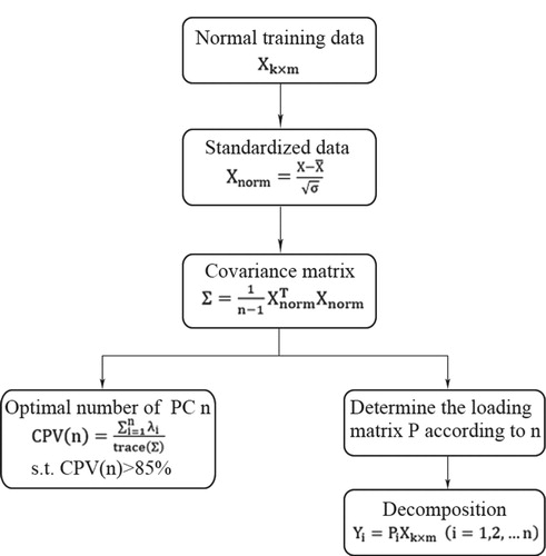
The basic steps of PCA analysis are the following steps:

1. Normalise the raw data set $X_{k\times m}$ (k is the feature number and m is the dimension) by the standard deviation: (1) $X_{norm}=\frac{X-\overline{X}}{\sqrt{\sigma }}$(1)

2. Calculate the covariance matrix ∑: (2) $\sum =\frac{1}{n-1}{X}_{norm}^T{X}_{norm}$(2)

3. Perform the singular value decomposition ∑ by (3) $\sum =V\mathrm{\Lambda }{V}^T$(3)

where $\mathrm{\Lambda }$ is a diagonal matrix that contains the eigenvalues (${\lambda }_i$) of the covariance matrix ∑ sorted in decreasing order (so₁ so₂ …  so_m) and the matrix $V$ are the eigenvectors of ∑.

1. Determine number n of principle components by cumulative percent variance. (4) $CPV=\frac{{\sum }_{i=1}^n{\lambda }_i}{trace(\sum )}$(4)

There are two ways to determine the number of principal elements, one is to select the eigenvalues greater than the value of one, and the other is the total variance contribution rate is greater than 85% (Kuhn 2007).

1. Determine the loading matrix $P$ according to the principle components ‘$n$’.

The PCA model divides the data matrix into two orthogonal complementary subspaces, including the principal component subspace (PCS) and the corresponding residual subspace (RS). Any vector can be decomposed into the sum of vectors composed of principal component subspaces and residual subspaces: (5) $\begin{array}{rl}X& =\hat{X}+\tilde{X}\end{array}$(5) (6) $\begin{array}{rl}\hat{X}& =P{P}^{T}X\in R_P\equiv \text{span}\{P\}\end{array}$(6) (7) $\begin{array}{rl}\tilde{X}& =(I-P{P}^T)X\in R_r\equiv \text{span}\{P{\}}^{\mathrm{\perp }}\end{array}$(7) where $\hat{X}$ is the PCS, it represents the correct direction of the measured vectors. $\tilde{X}$ represents the RS, it is the direction of faulty measurements. The two are mutually orthogonal. Therefore, we can establish the monitoring model of process monitoring in principal component space and residual space, in which the main element space reflects the measure of normal data change, RS mainly reflects the change of measure of the noise in the data.

2.2. Fault detection

The established PCA models, which using the historical data under normal operating condition, can be used to detect the dimensionality reduction of the sensor measurement data by subspace correlation. Statistics are used as fault indices, which will increase significantly to an abnormal level if sensor faults occur. There are two monitoring statistics methods: the Hotelling’s T²-statistic and Q-statistics or SPE (Alkaya and Eker 2011).

1. Q statistic

The full name of Q statistic is squared prediction error statistics (abbreviated as SPE). It can be seen from the name, the statistics reflects the change of sample data in its residual space, which is defined as follows: (8) $SPE=||X(I-P{P}^T)||<{\delta }_a^2$(8) the ${\delta }_a^2$ indicates the corresponding control limit when the confidence level is $\alpha$, and the control limit is calculated as follows: (9) ${\delta }_a^2={\theta }_1(1+\frac{c_a\sqrt{2{\theta }_2{h}_0^2}}{{\theta }_1}+\frac{{\theta }_2{h}_0(h_0-1)}{{\theta }_1^2}{)}^{\frac{1}{h_0}}$(9) where ${\theta }_i={\sum }_{i=n+1}^m{\lambda }_j^i,(i=1,2,3)$, $h_0=1-\frac{2{\theta }_1{\theta }_3}{3{\theta }_2^2}$; $\lambda$ is the covariance matrix eigenvalue of the matrix X, m is the dimension of the sample, and n is the number of the selected principal components. $c_a$ is the threshold of the standard normal distribution at the confidence level of $\alpha$.

Moreover, there is another control limit ${\delta }^2=g{\chi }_{\alpha }(h)$, where $g=\frac{{\theta }_2}{{\theta }_1}$,$h_1=\frac{{\theta }_1^2}{{\theta }_2}$,${\chi }_{\alpha }(h)$ is the critical value of the ${\chi }^2$ distribution with degrees of freedom as h and confidence level as $\alpha$. If the SPE exceeds the control limit, the correlation between the data was changed which means a fault has occurred.

1. Hotelling’s T² statistic

The Hotelling’s T² statistic reflects the change of the principal component space: (10) $T^2=XP{\mathrm{\Lambda }}^{-1}{P}^T{X}^T\le T_{\alpha }^2$(10) where $\mathrm{\Lambda }=diag\{{\lambda }_1,{\lambda }_2,\dots ,{\lambda }_n\}$, $T_{\alpha }^2$ represents the $T^2$ control limit with a confidence level of $\alpha$. Assuming that the normally running sample obeys a multivariate normal distribution, the control limit of the $T^2$ is computed as follows: (11) $T_{\alpha }^2=\frac{n(m-1)}{m-n}{F}_{\alpha }(n,m-n)$(11) where $F_{\alpha }(n,m-n)$ is a $F$ distribution with n and m-n degrees of freedom and confidence level of $\alpha$.

The PCA model judges if the $T^2$ and Q statistics exceed their corresponding control limits to determine whether the process is faulty or not. When the turbine is running in the normal condition, the $T^2$ and SPE of the master model are within the control limit, otherwise the $T^2$ and SPE statistics will exceed the control limit.

1. Hybrid indicator

Both $T^2$ and SPE statistics are used for the fault diagnosis of processes. As can be seen from the definition, the two spaces are orthogonal to each other, representing different aspects of the monitoring information, where the principal space contains the primary information of the samples, and the residual space contains mainly the noise information of the samples, so the $T^2$ control limit is usually larger than the SPE control limit. In the actual application process, in order to fully reflect the changes in the original data, we usually use the two together, while monitoring two different aspects of the industrial process.

Therefore, a hybrid indicator for fault detection is proposed, which is simpler and more convenient than using two indicators: (12) $\phi (x)=\frac{SPE(x)}{{\delta }_{\alpha }^2}+\frac{T^2(x)}{T_{\alpha }^2}=x^T\varphi x$(12) where (13) $\varphi =\frac{P{\mathrm{\Lambda }}^{-1}{P}^T}{T_{\alpha }^2}+\frac{I-P{P}^T}{Q_a^2}$(13) Notice that $\varphi$ is symmetric and positive definite.

The hybrid indicator is: (14) ${\xi }^2=g{\chi }_{\alpha }(h)$(14) where the coefficient g is given by (15) $g=\frac{\sum v_j{\lambda }_j^2}{\sum v_j{\lambda }_j^{}}=\frac{\text{trace}{(S\varphi )}^2}{\text{trace}(S\varphi )}$(15) and $h$ is given by (16) $h=\frac{(\sum v_j{\lambda }_j^{}{)}^2}{\sum v_j{\lambda }_j^2}=\frac{{[\text{trace}(S\varphi )]}^2}{\text{trace}{(S\varphi )}^2}$(16) ${\lambda }_j^{}$ is the jth eigenvalue of the matrix $S\varphi$ with a multitude $v_j$, where $S=\mathrm{cov}(X)$, If all of the eigenvalues are distinctive, then $v_j=1$. ${\chi }_{\alpha }$ is a $\chi$ distribution with a confidence level of $\alpha$. After $g$ and $h$ are calculated, the confidence limit of $\phi$ can be obtained. When $\phi (x)\le {\xi }^2$, we can think it in a normal working condition.

3. Experimental validation

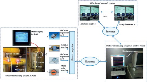
This experiment was made in a testing platform of steam turbine for marine application. The turbine system is an old one from power plant and used to generate electrical power. The platform is used to monitor the lubrication system under different conditions and evaluate its reliability. We deployed the oil online monitoring system on to the turbine machine lubricant system.

More than two thousand data are used in this study, which are the turbine oil monitoring parameters acquired from the experimental subject of steam turbine VG46 in a marine turbine reliability testing platform by the self-developed integrated online monitoring system. Here are three of the most important sensors. (i) ARGO-HYTOS LubCos H₂Oplus II Lubrication condition sensor records the following physical oil characteristics as well as its periodic change: Temperature, relative oil humidity and water activity, relative permittivity and conductivity of the fluid, respectively. As especially the conductivity and the relative permittivity show a strong connection to the temperature, next to the characteristic values at current temperature the sensor also sends the data at reference temperature. (ii) MEAS FPS2800B12C4 is an innovative fluid characteristic sensor which can directly and simultaneously measure the viscosity, density, dielectric constant and temperature of fluid. (iii) ARGO-HYTOS OPComII particle concentration monitoring sensor takes the sample fluid from one pipe to the inlet and enters the measuring space through a one-way valve. It can carry out second measurements and calculate iron filings. When the piston drained the sample fluid, it passed through the one-way valve in the other pipe. The plunger moves to the entrance when it is connected to the power supply. Piston movement and valve configuration result in pump movement to ensure that the oil sample is measured more than once. The measurement cycle takes about 80 s.

The three sensors are shown in Figure 2. The data acquisition module is shown in Figure 3 and the integrated online condition monitoring system is shown in Figure 4.

Figure 2. Three of the most important sensors.

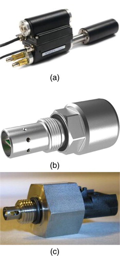
Figure 3. Sensors in the monitoring cabinet.

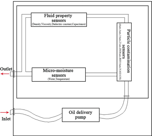
Figure 4. Overall design of the online condition monitoring system for lubricating oil.

Moreover, the data in Table 1 are a manifestation of the oil samples of the statistical change series of VG46 for nine months. The data have 15 indicators including power (x1), density (x2), viscosity (x3), dielectric constant (x4), temperature (x5), particle 4um (x6), particle 6um (x7), particle 14um (x8), particle 21um (x9), ISO6um (x10), ISO14um (x11), capacitance(x12), water (x13) and NAS1638 (x14). The vibration collected is a constant value, so we removed it.

Table 1. An example of data structure.

Power (Mw)	Density (g/cm³)	Viscosity (CST)	Dielectric constant	Temperature (°C)	4 um	6 um
333.3368	0.860	33.4620	2.185	38.3	140	31
14um	21um	ISO6um	ISO14um	Capacitance (pF)	Water (%)	NAS 1638
6	1	13	7	2.14	51.56	4

Empirically, there is a strong correlation between these parameters. Therefore, we use Python to analyse the correlation between the features, and Figure 5 is a correlation heatmap of the features obtained by Python.

Figure 5. Heatmap of the features correlation.

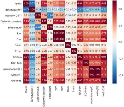
From the heatmap, we find that there is a great correlation between features. The PCA is used to reduce the dimensionality of the features consequently. The following experimental results obtained from PCA are analysed one by one.

The characteristic root and distribution of each principal component is shown in Figure 6 and the ratio of the characteristic root of each principal component and the proportion of each characteristic root is calculated, as shown in Table 2. From the last column in Table 2, we can see that the first 4 principal components of the root of the total proportion of the proportion of more than 85% (Kuhn 2007), therefore, taking the first 4 principal components to reflect the overall characteristics of the oil changes trend in the status can better represent the fourteen raw monitoring indicators.

Figure 6. Principal component scree plot.

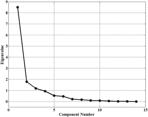
Table 2. Total variance explained.

	Initial eigenvalues			Extraction sums of squared loadings
Component	Total	% of variance	Cumulative %	Total	% of variance	Cumulative %
1	8.514	60.813	60.813	8.514	60.813	60.813
2	1.778	12.697	73.511	1.778	12.697	73.511
3	1.177	8.405	81.915	1.177	8.405	81.915
4	0.938	6.701	88.616	0.938	6.701	88.616
5	0.533	3.809	92.425
6	0.459	3.276	95.701
7	0.207	1.480	97.182
8	0.160	1.146	98.327
9	0.096	0.688	99.015
10	0.082	0.583	99.598
11	0.039	0.278	99.876
12	0.013	0.092	99.968
13	0.003	0.023	99.991
14	0.001	0.009	100.000

Meanwhile, the component matrix $P$ is also obtained, as shown in Table 3. Next, we constructed the fault monitoring system. The flow chart of fault monitoring is shown in Figure 7.

Figure 7. Flow chart of fault monitoring.

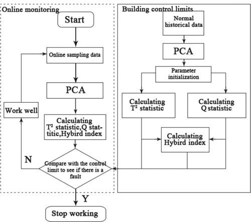
Table 3. Component matrix.

	Component
	1	2	3	4
Power	0.937	0.072	−0.024	−0.022
Density (g/cm^3)	−0.903	0.084	0.099	−0.004
viscosity(CST)	0.158	−0.939	0.183	−0.122
Dielectric constant	0.985	−0.065	−0.058	−0.002
Temperature (°C)	0.461	0.820	−0.220	0.112
4um	0.936	−0.195	−0.088	0.050
6um	0.956	−0.166	−0.075	0.037
14um	0.150	0.347	0.621	−0.624
21um	0.113	0.058	0.667	0.712
ISO6um	0.938	0.060	0.020	−0.063
ISO14um	0.667	0.123	0.438	−0.079
Capacitance (pF)	0.891	−0.003	−0.119	0.004
Water (%)	0.893	−0.017	−0.115	0.002
NAS1638	0.935	0.005	0.133	0.025

Take the confidence level $\alpha$ as 99%, which means that one alarm in every 100 data can typically be expected and the corresponding control limit is shown in Table 4.

Table 4. Monitoring index and its control limit.

Confidence level equals 99%
Monitoring index	$T^2$	Q (SPE)	Hybrid indicator
Values	18.096	3.615	1.702

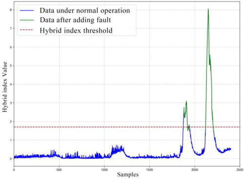
After doing the aforementioned work, we used the constructed control limits to test their performance. The working load of the steam turbine varies between 310 and 600 MW, but it mostly works below 550 MW. During the operation of the steam turbine, we raised its power to the maximum critical value which is close to 600 MW, and added one fault by stopping the oil filter at the same time after 06h30 and 11h05 on 6 April. This time point is the time point when the fault occurs. The corresponding serial numbers of the beginning of the fault are 1880 and 2120. For the purpose of facilitating the analysis, we put the two-sample sequence collected after adding fault together to plot. And the following three monitoring charts are obtained:

From Figures 8–10, because of the system delay, the three monitoring indexes begin to increase rapidly from the 1840th samples. They all responded well to the worsening trend after adding fault. In actual observation, 1880th to 1915th and 2125th to 2165th samples are considered to be collected under the condition of fault.

Figure 8. $T^2$ index monitoring trends.

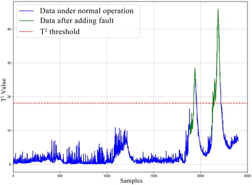
Figure 9. $Q$ index monitoring trends.

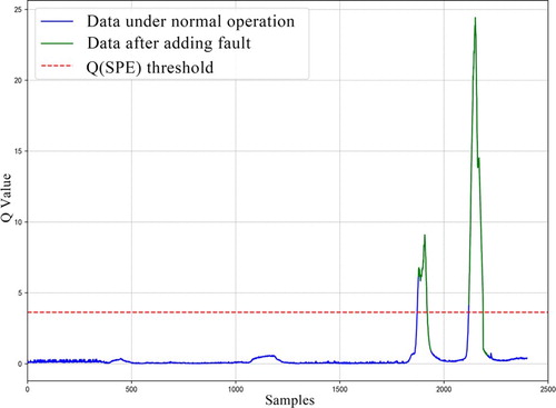
Figure 10. Hybrid indicator monitoring trends.

Quantitative analysis of the relationship between them, the false alarm rate of each index at the beginning and end of the fault is recorded respectively, and the results are shown in Table 5 and Figure 11.

Figure 11. False alarm rate of statistical indicators.

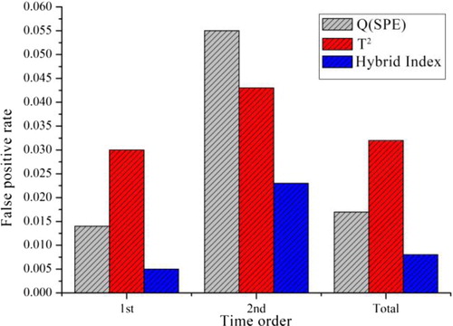
Table 5. False alarm rate of statistical indicators.

	Fault occurred 1st time	Fault stopped 1st time	False alarm rate 1st time	Fault occurred 2nd time	Fault stopped 2nd time	False alarm rate 2nd time	Total false alarm rate
Actual value	1880	1940	–	2120	2210	–	–
$T^2$ index	1925	1955	0.030	2131	2216	0.043	0.017
Q index	1872	1920	0.014	2119	2189	0.055	0.032
Hybrid indicator	1874	1943	0.005	2121	2208	0.023	0.008

As can be seen from Table 5 and Figure 11, whenever the fault shows up in the beginning or in the end on monitoring, hybrid indicator has greater advantages. When determining whether the fault occurs and ends, it ensures the accuracy, and also leaves the remaining margin at the same time. Thus the operator can adjust the working status of the turbine in a timely manner.

4. Conclusion

In this paper, for the shortage of the traditional PCA multivariate monitoring method, this paper uses a hybrid monitoring indicator of combined the traditional Hotelling’s T² and Q statistic for fault prediction, which not only avoids the simple use of single fault monitoring that may cause the fault to the diagnosis, but also simplifies the fault prediction model. A new data preprocessing technique and a new fault detection scheme designed for Hotelling’s T² and SPE and their hybrid indicator are presented, which are suitable for the detection of turbine lubrication system faults. The method in the paper can extract fault information and reduce the effect of noises and disturbances effectively on faults detection. Early warning can be provided to the operators through the proposed monitoring approach.

Disclosure statement

No potential conflict of interest was reported by the authors.

ORCID

Biao Hu http://orcid.org/0000-0002-1359-7403

Reza Malekian http://orcid.org/0000-0002-2763-8085

Zhixiong Li http://orcid.org/0000-0002-7265-0008

Additional information

Funding

This paper is sponsored by the grants from the National Natural Sciences Foundation of China (NSFC) [No. 51309185] and [No. 5197090691] .

References

- Ahmadi H, Mollazade K. 2009. A practical approach to electromotor fault diagnosis of imam khomaynei silo by vibration condition monitoring. Afr J Agric Res. 4(4):383–388.
- Alkaya A, Eker I. 2011. Variance sensitive adaptive threshold-based pca method for fault detection with experimental application. ISA Trans. 50(2):287–302. doi: 10.1016/j.isatra.2010.12.004
- Bakdi A, Kouadri A. 2017. A new adaptive PCA based thresholding scheme for fault detection in complex systems. Chemom. Intell. Lab. Syst. 162:83–93. doi: 10.1016/j.chemolab.2017.01.013
- Cheng J, Yang Y, Yang Y. 2012. A rotating machinery fault diagnosis method based on local mean decomposition. Digit Sig Process. 22(2):356–366. doi: 10.1016/j.dsp.2011.09.008
- Dunia R, Qin SJ, Edgar TF, Mcavoy TJ. 2010. Identification of faulty sensors using principal component analysis. AIChE J. 42(10):2797–2812. doi: 10.1002/aic.690421011
- Gharavian MH, Ganj FA, Ohadi AR, Bafroui HH. 2013. Comparison of fda-based and pca-based features in fault diagnosis of automobile gearboxes. Neurocomputing. 121(18):150–159. doi: 10.1016/j.neucom.2013.04.033
- Gresham RM. 2008. Machinery oil analysis-methods, automation & benefits: a guide for maintenance managers, supervisors & technicians, third edition. Tribol Lubr Technol. 65:1–61.
- Joe QS. 2010. Statistical process monitoring: basics and beyond. J Chemom. 17(8–9):480–502.
- Katnam KB, Comer AJ, Roy D, Silva LFM, Young TM. 2015. Composite repair in wind turbine blades: an overview. J Adhes. 91(1–2):113–139. doi: 10.1080/00218464.2014.900449
- Kuhn D. 2007. Reasoning about multiple variables: control of variables is not the only challenge. Sci Educ. 91(5):710–726. doi: 10.1002/sce.20214
- Loutas TH, Roulias D, Pauly E, Kostopoulos V. 2011. The combined use of vibration, acoustic emission and oil debris on-line monitoring towards a more effective condition monitoring of rotating machinery. Mech Syst Sig Processing. 25(4):1339–1352. doi: 10.1016/j.ymssp.2010.11.007
- Peng Z, Kessissoglou NJ, Cox M. 2005. A study of the effect of contaminant particles in lubricants using wear debris and vibration condition monitoring techniques. Wear. 258(11–12):1651–1662. doi: 10.1016/j.wear.2004.11.020
- Roylance BJ, Williams JA, Dwyer-Joyce R. 2000. Wear debris and associated wear phenomena – fundamental research and practice. Proc Inst Mech Eng Part J J Eng Tribol. 214(1):79–105. doi: 10.1243/1350650001543025
- Sun X, Marquez HJ, Chen T, Riaz M. 2005. An improved pca method with application to boiler leak detection. ISA Trans. 44(3):379–397. doi: 10.1016/S0019-0578(07)60211-0
- Xu XJ, Yan XP, Sheng CX. 2016. Non-destructive online condition monitoring and trend prediction of lubricating oil in a steam turbine. Fail Diagn. 58(1):1–4.
- Zhang PL, Xu C, Ren GQ, Fu JP, Li B. 2010. Prediction of wear condition of internal combustion engine based on multi-dimensional time series model. Lubr Sealing. 35(6):37–40. Chinese.
- Zhao JG, Chen HS, Liu XF, Huang HW, Jiang JJ. 2011. Research on the technology of on-line monitoring and self-maintenance of oil liquid state. Hydraul Pneumatic. 3:32–34. Chinese.