A numerical study on flow field and maneuvering derivatives of KVLCC2 model at drift condition

ABSTRACT

This paper investigates the flow field around the KRISO Very Large Crude Carrier (KVLCC2) model at different drift angle using the RANS method in combination with the Re-Normalization Group (RNG) $k-\epsilon$ and Shear Stress Transport (SST) $k-\omega$ turbulence models. The hydrodynamic forces and yaw moment acting on the KVLCC2 model are calculated under the different turbulence models and drift angles, and the numerical results are compared with previous experimental results. The accuracy of the numerical results is found to be acceptable, especially under the SST $k-\omega$ turbulence model. Three different mesh conditions are employed to perform the verification and validation based on the methodology and procedures suggested by ITTC. The surface pressure distribution, vorticity distribution, and surface flow features around the hull are observed and analysed. The maneuvering derivatives are calculated based on numerical results to create the mathematic model of ship maneuvering motions in the marine simulator and predict the ship maneuvering motions.

1. Introduction

In recent years, an increasing number of very large crude carriers (VLCCs) have been built by ship owners in an attempt to reduce the costs of transporting crude oil around the world. Compared with other ships, it is somewhat difficult to maneuver VLCCs (Wu et al. 2005). Hence, maneuverability is a key component in the performance of VLCC designs. The ‘temporary standard of ship maneuverability’ and ‘standard for ship maneuverability’ are promulgated by the International Maritime Organization (IMO), but these standards cannot ensure the absolute navigation safety of VLCCs. For this purpose, the KVLCC2 hull is used as a benchmark model tanker by the ITTC Maneuvering Technical Committee in comparative studies of ship maneuverability, and it is essential to study the maneuverability and vorticity flow field around the hull of VLCCs. The model test in the tank is widely used to study the ship’s maneuverability. In the test process, the technology of particle image velocimetry (PIV) can be employed to monitor the physical information of the disturbed flow field and visualise the flow field around the ship (Wang et al. 2017). The test process is complex and the distribution information of the flow field around the ship obtained from the test is limited. Compared with traditional methods, computational fluid dynamics (CFD) method can provide more detailed information of vorticity flow around the ship and propeller plane by way of various visualisation methods. Stern et al. (2015) give an overview of modelling, numerical methods, and high-performance computing for naval architecture and ocean engineering by CFD method. CFD has been an effective method for studying the ship maneuverability and its vorticity flow field.

In recent decades, a series of numerical studies on KVLCC2 have been carried out by way of different CFD codes and turbulence models. Most research used the RANS method to study the forces and moments involved in planar motion mechanism (PMM) maneuvers. Turnock et al. (2008) investigated the global forces and moments acting on the KVLCC2 hull form undergoing straight line, drift, and pure sway PMM tests. Yasukawa and Yoshimura (2015) introduced a MMG standard method. Maneuvering simulations were carried out for KVLCC2 model and full scale ship for validation of the method. Van Hoydonck et al. (2019) performed research on ship-bank interaction effects in which viscous flow solvers were used to predict the hydrodynamic forces and moments on the ship. He et al. (2016) utilised the commercial StarCCM+ CFD software to carry out oblique resistance and PMM simulations for the MOERI KVLCC2, and obtained the linear maneuvering derivatives of the pure sway and pure yaw motions. Abbas and Kornev (2016) performed the computations of integral forces, surface pressure distribution and the wake behind the KVLCC2 tanker under simple manoeuvring (drift angles 6° and 12°) and complex manoeuvring (drift angle and yaw rate of 0.2, 0.4 and 0.6) conditions. The results were compared with experimental results. Park et al. (2015) carried out uncertainty analysis for added resistance experiment of KVLCC2 ship. Pereira et al. (2017) presented the quantification of numerical and modelling errors for the solution of the flow around the KVLCC2 tanker at model-scale Reynolds number. Yang et al. (2019) performed a numerical study on the hydrodynamic performance of the semi-spade rudder and KP458 propeller of the KVLCC2 model tanker. Fureby et al. (2016) investigated the flow around the KVLCC2 model tanker hull at 0°, 12° and 30° drift using classical Reynolds Averaged Navier–Stokes (RANS) models from two different proprietary codes, hybrid RANS-LES models from one of these proprietary codes, and Large Eddy Simulation (LES) models from a third semi-proprietary code. Feng et al. (2015) conducted a numerical simulation of the viscous flow around a KVLCC2 model appended with a rudder moving at different drift angle by solving the RANS equations in conjunction with a RNG k-ε turbulence model. The motions and added resistance of KVLCC2 at Froude numbers of 0.142 and 0.25 with free and fixed surges in short and long head waves have been predicted using unsteady RANS and validated against experimental fluid dynamics (EFD) (Sadat-Hosseini et al. 2013). For KVLCC2, different experimental data were obtained for 0°, 6°, and 12° drift angle (Kume et al 2006) or for different drift angles, water depths, and basin wall effects (Wang et al. 2009; Toxopeus et al. 2013). Xing et al. (2012) examined the flow past the KVLCC2 model using detached eddy simulations at drift angles of 0°, 12°, and 30°. The influence of ship model size on the maneuvering hydrodynamic coefficients has also been investigated, and the hydrodynamic forces and yaw moment on the KVLCC2 model have been predicted for a static drift and a pure sway test and validated against benchmark model scale test data (Jin et al. 2016). For KVLCC2M, and the similar KVLCC2 configurations, the unsteady viscous flow in both deep and shallow water has been simulated, and the hydrodynamic forces, surface pressure distribution, and wake field have been determined by solving the unsteady RANS equations in combination with the k-ω shear-stress transport (SST) turbulence model. The overset mesh technology can be used in simulations to avoid any mesh distortion at large drift angle (Meng and Wan 2016). However, relatively little research has considered the vorticity flow around the vessel, which is closely related to resistance and noise.

In the present study, the flow field around KVLCC2 is simulated in oblique motion at drift angles of 0°, 3°, 6°, 9° and 12° using the RANS method in order to comparing them with experimental results from a towing tanker (Kume et al. 2006). Three different sets of mesh (coarse, medium and fine) are adopted to perform the verification and validation. The RNG $k-\epsilon$ and SST $k-\omega$ turbulence models are employed to study the effect of turbulence models on the numerical simulations. The lateral force and yaw moment are calculated under different drift angles and turbulence models. The numerical results are compared against experimental results. The surface pressure and vorticity distribution around the hull are observed and analysed. The maneuvering derivatives are calculated based on the numerical results. It is an attempt to predict the ship maneuvering motions in the marine simulator by way of CFD technology.

2. Mathematical model

2.1. RNG $k-\epsilon$ turbulence model

The RNG $k-\epsilon$ model is derived from the instantaneous Navier–Stokes equations using a mathematical technique called ‘renormalization group’ methods (Yakhot and Orzag 1986). Compared with the standard $k-\epsilon$ model, the RNG form includes an additional term that improves the accuracy for rapidly strained flows in its $\epsilon$ equation and considers the effect of swirl on turbulence to improve the accuracy for swirling flows. An analytical formula for turbulent Prandtl numbers is also provided, as well as an analytically derived differential formula for effective viscosity that accounts for low Reynolds number effects. The transport equations for the RNG $k-\epsilon$ model are expressed as (1) $\begin{array}{rl}\frac{\mathrm{\partial }(\rho k)}{\mathrm{\partial }t}+\frac{\mathrm{\partial }(\rho k{u}_i)}{\mathrm{\partial }{x}_i}& =\frac{\mathrm{\partial }}{\mathrm{\partial }{x}_j}[a_k{\mu }_{eff}\frac{\mathrm{\partial }k}{\mathrm{\partial }{x}_j}]+G_k-\rho \epsilon \end{array}$(1) (2) $\begin{array}{rl}\frac{\mathrm{\partial }(\rho \epsilon )}{\mathrm{\partial }t}+\frac{\mathrm{\partial }(\rho \epsilon u_i)}{\mathrm{\partial }{x}_i}& =\frac{\mathrm{\partial }}{\mathrm{\partial }{x}_j}[a_{\epsilon }{\mu }_{eff}\frac{\mathrm{\partial }\epsilon }{\mathrm{\partial }{x}_j}]\\ & +\frac{C_{1\epsilon }^{\ast }\epsilon }{k}{G}_k-C_{2\epsilon }\rho \frac{{\epsilon }^2}{k}\end{array}$(2) where k is the turbulent kinetic energy, $\epsilon$ is the dissipation rate, ${\mu }_{eff}=\mu +{\mu }_t$, ${\mu }_t=\rho C_{\mu }(k^2/\epsilon )$, $C_{\mu }=0.0845$, $a_k=a_{\epsilon }=1.39$, $C_{1\epsilon }^{}=1.42$, $C_{2\epsilon }=1.68$, $\beta =0.012$, ${\eta }_0=4.377$, $C_{1\epsilon }^{\ast }=C_{1\epsilon }-(\eta (1-\eta /{\eta }_0)/1+\beta {\eta }^3)$, and $\eta =(2E_{ij}\cdot E_{ij}{)}^{1/2}(k/\epsilon )$.

2.2. SST $k-\omega$ turbulence model

The SST $k-\omega$ turbulence model (Menter 1994) is a two equation eddy viscosity model. It is the model of choice in the sub layer of the boundary region. It does not involve damping functions and allows simple Dirichlet boundary conditions to be specified. The SST formulation also switches to a $k-\epsilon$ behaviour in the free-stream, and thereby avoids the common $k-\omega$ problem of being too sensitive to the free-stream turbulence properties at the inlet. The SST $k-\omega$ model can overestimate the turbulence levels in regions with large normal strain, such as stagnation regions and regions with strong acceleration. However, this tendency is much less pronounced than with a normal $k-\epsilon$ model. The SST $k-\omega$ turbulence model is expressed as (3) $\begin{array}{rl}\frac{\mathrm{\partial }k}{\mathrm{\partial }t}+u_i\frac{\mathrm{\partial }k}{\mathrm{\partial }{x}_i}& =\frac{\mathrm{\partial }}{\mathrm{\partial }{x}_j}[(\nu +{\sigma }_k{\nu }_t)\frac{\mathrm{\partial }k}{\mathrm{\partial }{x}_j}]+{\tilde{P}}_k-{\beta }^{\ast }k\omega +S_k\end{array}$(3) (4) $\begin{array}{rl}\frac{\mathrm{\partial }\omega }{\mathrm{\partial }t}+u_i\frac{\mathrm{\partial }\omega }{\mathrm{\partial }{x}_i}& =\frac{\mathrm{\partial }}{\mathrm{\partial }{x}_j}[(\nu +{\sigma }_k{\nu }_t)\frac{\mathrm{\partial }\omega }{\mathrm{\partial }{x}_j}]+a{S}^2\\ & -\beta {\omega }^2+2(1-F_1){\sigma }_{\omega 2}\frac{1}{\omega }\frac{\mathrm{\partial }k}{\mathrm{\partial }{x}_j}\frac{\mathrm{\partial }\omega }{\mathrm{\partial }{x}_j}+S_{\omega }\end{array}$(4) Where k is the turbulent kinetic energy, ω is the turbulence specific dissipation rate, ${\sigma }_k=\frac{1}{F_1/{\sigma }_{k1}+(1-F_1)/{\sigma }_{k2}},{\nu }_t=\frac{a_{1}k}{max(a_1\omega ,\mathrm{\Omega }{F}_2)}$ $\begin{array}{rl}{\tilde{P}}_{\kappa }& =min[{\nu }_t\frac{\mathrm{\partial }{u}_i}{\mathrm{\partial }{x}_j}(\frac{\mathrm{\partial }{u}_i}{\mathrm{\partial }{x}_j}+\frac{\mathrm{\partial }{u}_j}{\mathrm{\partial }{x}_i}),10{\beta }^{\ast }\rho k\omega ],\\ {\sigma }_{\omega }& =\frac{1}{F_1/{\sigma }_{\omega 1}+(1-F_1)/{\sigma }_{\omega 2}}\end{array}$The blending functions $F_1$, $F_2$ can be described as $F_1=\tan ({\mathrm{\Phi }}_1^4)$, $F_2=\tan ({\mathrm{\Phi }}_2^2)$, $a_1=0.555$, $a_2=0.44$, ${\beta }_1=0.075$, ${\mathrm{\Phi }}_1=min[max(\frac{\sqrt{k}}{{\beta }^{\ast }\omega y},\frac{500\nu }{y^2\omega }),\frac{4\rho {\sigma }_{\omega 2}k}{C{D}_{k\omega }{y}^2}]$, $C{D}_{k\omega }=max[2\rho {\sigma }_{\omega 2}\frac{1}{\omega }\frac{\mathrm{\partial }k}{\mathrm{\partial }{x}_j}\frac{\mathrm{\partial }\omega }{\mathrm{\partial }{x}_j},{10}^{-10}]$, ${\beta }_2=0.0828$, ${\mathrm{\Phi }}_2=max[\frac{2\sqrt{k}}{{\beta }^{\ast }\omega y},\frac{500\nu }{y^2\omega }]$, ${\sigma }_{k1}=0.85$, ${\sigma }_{k2}=1$, ${\sigma }_{\omega 1}=0.5$, and ${\sigma }_{\omega 2}=0.856$.

3. Benchmark model and computation design

3.1. Benchmark model

The KVLCC2 model is selected as the test model in this study. This is the second variant of the MOERI tanker, with more U-shaped stern frame lines, and represents a typical 300,000 ton oil tanker. In recent years, the KVLCC2 hull form has been selected as the benchmark test case for a series of workshops investigating ship hydrodynamics and maneuverability. These workshops supplied a large amount of experimental and numerical data that can be used to validate numerical results (Kume et al. 2006). The test model moves with a speed U = 0.994 m/s in calm water at drift angles of 0°, 3°, 6°, 9° and 12°.

The Froude number and Reynolds number are defined as (5) $\begin{array}{rl}{F}_r& =\frac{U}{\sqrt{gL}}\end{array}$(5) (6) $\begin{array}{rl}{R}_e& =\frac{UL}{\nu }\end{array}$(6) Where $U$ is the ship velocity, $L$ is the ship length, $g$ is acceleration due to gravity, and $\nu$ is the kinematic viscosity.

We consider a Froude number of 0.142 and Reynolds number of 3.945 × 10⁶ in computations using the ANSYS FLUENT software solver. The specifics of the KVLCC2 hull form are presented in Figure 1. The main parameters of the full and model scale KVLCC2 are listed in Table 1.

Figure 1. The KVLCC2 hull form with the main particulars.

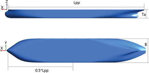
Table 1. Main particulars of KVLCC2 in full and model scale.

Description	Symbol	Full scale	Model scale	Unit
Length between perpendiculars	LPP	320.0	4.9700	m
Breadth of waterline at designed draft	Bw1	58.0	0.9008	m
Depth molded	D	30.0	0.4659	m
Draught	T	20.8	0.3231	m
Displacement volume molded	–	312,622	1.1712	m^3
Wetted surface area bare hull	Swa	27,194	6.5597	m^2
Block coefficient	Cb	0.8098	0.8098	–
Midship section coefficient	Cm	0.9980	0.9980	–
Center of buoyancy forward of midship	LCB	3.48	3.48	%Lpp
Length-breadth ratio	L/B	5.517	5.517	–
Breadth-Draught ratio	B/T	2.788	2.788	–
Length-Draught ratio	L/T	15.385	15.385	–

3.2. Numerical set-up and mesh generation

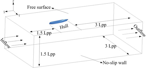
The geometry and details of the boundaries are shown in Figure 2. The right-handed Cartesian coordinate system is used to fix the computational domain and the KVLCC2 hull. The origin is located at the intersection of the stern with the design water-plane and the ship centre plane. The x-axis runs along the direction of longitude at the mid-section and points to the bow, the z-axis lies vertical to the water-plane, and the y-axis runs along the mid-ship section and points to the port side. According to Equation (5), the inlet velocity is set to a low velocity U = 0.994 m/s by Froude number of 0.142. The velocity inlet is used for inlet condition. The out-flow outlet is used for outlet condition. The no-slip wall boundary condition is imposed on the bottom and sides of computational domain and the hull surface. The influence of wave-making can be neglected due to the small Froude number. So the symmetric condition is set for the undisturbed free surface (Tian et al. 2010).

Figure 2. Computational domain and boundary conditions.

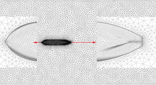
A hybrid mesh is generated using a top-down robust method by ICEM software. The mesh is refined around the bow, stern, and bilge. The curves around bow or stern with a high curvature are refined. The boundary layer affects the distribution of the pressure near the hull surface, so the thickness of the boundary layer must conform to the turbulence model, that is, the distance from the hull surface to the cells in the first layer of the mesh must be reasonable for the turbulence model used. The y⁺ value is set to 52 for the boundary layer around the hull surface. The total number of cells in the whole computational domain is approximately 0.7 million. The mesh around the hull surface and the division of the computational domain are shown in Figures 3 and 4, respectively.

Figure 3. Ship hull surface meshes.

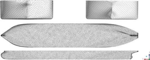
Figure 4. Mesh divisions of computational domain and boundary layer.

4. Numerical results and discussion

Numerical simulations of the flow past the KVLCC2 model are conducted with the prescribed oblique motion at drift angles of 0°, 3°, 6°, 9° and 12°. Two turbulence models are used in the numerical simulations. The hydrodynamic forces X, Y and moment N are obtained at each drift angle and for both turbulence models. To compare them with the experimental results from a towing tanker, these quantities are expressed by the dimensionless coefficients (Wang et al. 2009) C_X, C_Y, and C_N, which can be calculated as (7a) $\begin{array}{rl}{C}_X& =\frac{X}{\frac{1}{2}\rho U^{2}Ld}\end{array}$(7a) (7b) $\begin{array}{rl}{C}_Y& =\frac{Y}{\frac{1}{2}\rho U^{2}Ld}\end{array}$(7b) (7c) $\begin{array}{rl}{C}_N& =\frac{N}{\frac{1}{2}\rho U^{2}Ld}\end{array}$(7c)

Where X and Y are the hydrodynamic forces, and N is the moment, and $\rho$ is the water density, and U is the velocity, and L is the ship length, and d is the ship draft.

4.1. Verification and validation

Numerical computation is carried out with the SST $k-\omega$ turbulence model at different drift angles. Uncertainty analysis is performed based on the methodology and procedures suggested by ITTC . Three different sets of mesh (coarse, medium and fine) are adopted in the verification and validation process. The refinement ration of fine to medium (medium to coarse) mesh is $\sqrt{2}$. Mesh quantity, hydrodynamic forces and moment coefficient at drift angle of 6° are listed in Table 2. At the medium mesh resolution, the computational data are stable and very similar to the data obtained under the fine mesh condition. That is, the computational results are relatively insensitive to the mesh resolution. The solutions (0 < R_G<1) exhibit the monotonic convergence condition for three different meshes in Table 3. The validation uncertainty for C_X, C_Y and C_N are 6.8%D, 12.5%D and 7.4%D respectively, where D is experimental data. The absolute value of comparison error E for C_X, C_Y and C_N are 4.5%D, 10.3%D and 6.4%D respectively, which are smaller than the validation uncertainty U_V. The validation is successful at the present U_V level. On the basis of these results, the following analysis of the flow field and calculation of maneuvering derivatives are performed using the computational data obtained under the medium mesh condition.

Table 2. Hydrodynamic force and moment coefficient (SST $k-\omega$) with different mesh quantity at drift 6°.

Mesh	Quantity	$C_X$(6°)	$C_Y$(6°)	$C_N$(6°)
Coarse(3)	372,935	−0.01926	0.02189	0.01607
Medium(2)	705,593	−0.01867	0.02277	0.01491
Fine(1)	1,372,623	−0.01852	0.02296	0.01482

Table 3. Verification and validation for hydrodynamic force and moment coefficient (SST $k-\omega$) at drift 6°.

Parameter	ε21	ε32	RG	PG	UV(%D)	|E|(%D)	D(Exp.)
CX	−0.00015	−0.00059	0.254	3.953	6.8	4.5	−0.01771
CY	−0.00019	−0.00088	0.216	4.425	12.5	10.3	0.0256
CN	0.00009	0.00116	0.078	7.379	7.4	6.4	0.01392

4.2. Hydrodynamic forces and moment

The numerical results are validated by comparing them with experimental results from a towing tanker. Data for drag X and coefficient C_X are listed in Table 4. A comparison of the drag coefficient under different turbulence models is shown in Figure 5. The numerical results for the drag coefficient C_X are in good agreement with the experimental results. Compared with the numerical results under the RNG $k-\epsilon$ turbulence model, the SST $k-\omega$ turbulence model is closer to the experimental results, with a maximum deviation of 8.7%. Data for lift Y and coefficient C_Y are listed in Table 5. A comparison of the lift coefficient under different turbulence models is shown in Figure 6. The numerical results for the lift coefficient C_Y under the different turbulence models exhibit a similar tendency as the experimental results. Data for moment N and coefficient C_N are listed in Table 6. The moment coefficient under different turbulence models is compared in Figure 7. The numerical results for the moment coefficient C_N are in good agreement with the experimental results. The numerical results are closer to the experimental results under the SST $k-\omega$ turbulence model. The deviation increases with the drift angle, reaching 7.6% at a drift angle of 12°.

Figure 5. The drag coefficients under different turbulence model and drift angles.

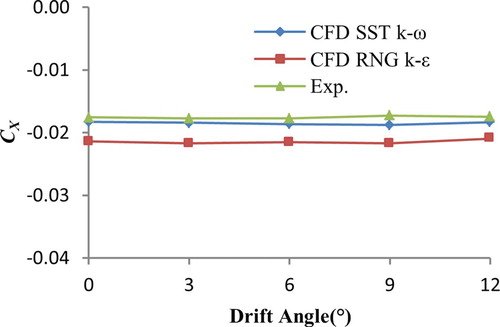
Figure 6. The lift coefficients under different turbulence model and drift angles.

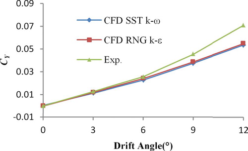
Figure 7. The moment coefficients under different turbulence model and drift angles.

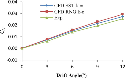
Table 4. Data for the drag X and coefficient$C_X$.

Drift	X	X	$C_X$	$C_X$	$C_X$
Angle	(CFD SST $k-\omega$)	(CFD RNG $k-\epsilon$)	(CFD SST $k-\omega$)	(CFD RNG $k-\epsilon$)	(Exp.)
0	−14.51325	−16.97344	−0.01830	−0.02140	−0.01756
3	−14.58745	−17.19769	−0.01839	−0.02169	−0.01776
6	−14.80823	−17.07280	−0.01867	−0.02153	−0.01771
9	−14.90506	−17.18169	−0.01879	−0.02167	−0.01729
12	−14.54437	−16.61814	−0.01834	−0.02095	−0.01750

Table 5. Data for the lift Y and coefficient $C_Y$.

Drift	Y	Y	$C_Y$	$C_Y$	$C_Y$
Angle	(CFD SST $k-\omega$)	(CFD RNG $k-\epsilon$)	(CFD SST $k-\omega$)	(CFD RNG $k-\epsilon$)	(Exp.)
0	0.39418	−0.16462	0.00050	−0.00021	−0.00004
3	8.90033	9.36576	0.01122	0.01181	0.01263
6	18.05769	19.06710	0.02277	0.02404	0.02560
9	29.74826	30.69911	0.03751	0.03871	0.04553
12	42.45993	43.31154	0.05354	0.05461	0.07082

Table 6. Data for the moment N and coefficient $C_N$.

Drift	Moment	Moment	$C_N$	$C_N$	$C_N$
Angle	(CFD SST $k-\omega$)	(CFD RNG $k-\epsilon$)	(CFD SST $k-\omega$)	(CFD RNG $k-\epsilon$)	(Exp.)
0	0.86389	0.14171	0.00022	0.00004	−0.00006
3	29.07491	30.93208	0.00738	0.00785	0.00612
6	58.75699	62.35089	0.01491	0.01582	0.01392
9	84.33274	90.28896	0.02140	0.02291	0.01940
12	107.64118	115.52808	0.02731	0.02931	0.02539

4.3. Surface pressure distributions

Figures 8 and 9 compare the surface pressure distribution between the experimental and numerical results at 6° and 12° drift angles, respectively. The surface pressure is expressed in the dimensionless coefficient (8) $C_p=\frac{P}{\frac{1}{2}\rho U^2}$(8) Where $P$ is the surface pressure of the hull, and $\rho$ is the water density, and U is the ship velocity.

Figure 8. Distribution of surface pressure at $\beta ={\text{6}}^{\circ }$.

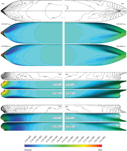
Figure 9. Distribution of surface pressure at $\beta ={12}^{\circ }$.

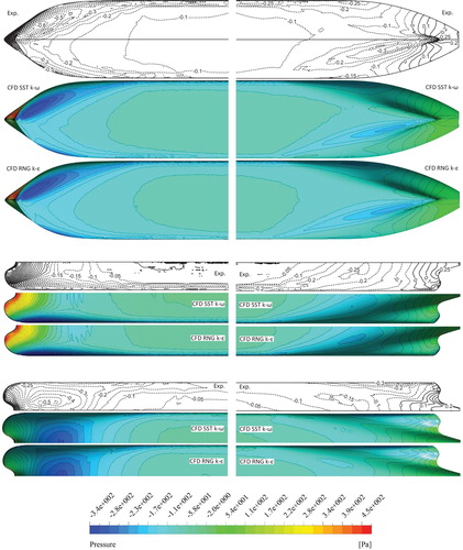
By comparing the numerical results for the surface pressure distribution under different turbulence models with experimental results, it is apparent that the numerical results are in good agreement with the experimental results, and that the SST $k-\omega$ turbulence model is closer to the experimental output. Figures 8 and 9 illustrate that there are two obvious low-pressure regions, one on the port side around the bow and one on the starboard side around the stern. The pressure distributions of both sides around the middle of the hull are nearly same with each other. The flow around the large curvature of the hull accelerates to produce the low-pressure regions. The pressure difference of the bow and stern produces a yaw moment, which turns the hull to the starboard side. From the figures, it can be seen that the pressure difference around the bow is greater than that around the stern, so the total lateral force points to the starboard side. As the drift angle increases, the pressure difference around the bow increases faster than that of the stern, so the lateral force increases with the drift angle.

4.4. Time-averaged vorticity flow

The vorticity structures are identified by the Q-criterion (Hunt et al. 1988), which is based on the second invariant of the velocity gradient tensor. However, the Q-criterion cannot be used to visualise the orientation of the detected vortex. To overcome this disadvantage, the flow is visualised using iso-surfaces of the dimensionless Q-criterion (Degani et al. 1990, Kamkar et al. 2010) according to the helicity (9) $H_n=\frac{v\cdot \omega }{|v||\omega |}$(9) Where $v$ is the velocity and $w$ is the vorticity vector. The Q-value is defined as (10) $Q=\frac{1}{2}({||W||}^2-{||D||}^2)$(10) Where $W$ and $D$ are the rotation tensors and rate-of-strain, respectively.

The Figures 10 and 11 illustrate the vorticity distribution around the hull under different turbulence models and drift angles. The figures present visualisations of Q-criterion, coloured by velocity, from the bilge. It can be seen that the vorticity distributions predicted under the RNG $k-\epsilon$ and SST $k-\omega$ turbulence model are similar in general, with minor differences. However, the simulation with the SST $k-\omega$ turbulence model can present more detailed vorticity distributions than the RNG $k-\epsilon$ turbulence model. The fore-body bilge vortex can be observed obviously in the simulation with the SST $k-\omega$ turbulence model. The Figures 5 and 7 also present that the drag and moment coefficients (C_X and C_N) calculated based on the SST $k-\omega$ turbulence model are closer to the experimental results. The low-Reynolds number effects, compressibility, and shear flow spreading are considered in the standard $k-\omega$ turbulence model. The SST $k-\omega$ turbulence model is designed to be one in the near-wall region, which activates the standard $k-\omega$ model, and zero away from the surface, which activates the transformed $k-\epsilon$ model. So, the results of hydrodynamic force and vorticity distribution indicate that the SST $k-\omega$ turbulence model is more suitable for the simulation of the flow field around the ship with a certain drift angle.

Figure 10. Representation of the vorticity by means of the Q criteria at Q = 0.02, with the RNG $k-\epsilon$ turbulence model.

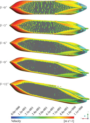
Figure 11. Representation of the vorticity by means of the Q criteria at Q = 0.02, with the SST $k-\omega$ turbulence model.

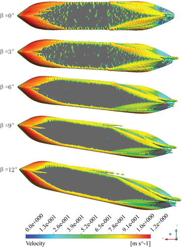
The simulation in Figures 10 and 11 captures the basic flow structure which includes fore-body bilge vortex, fore-body side vortex, aft-body bilge vortex, and aft-body side vortex at different drift angle. At 0° drift, the predictions show that a pair of bilge vortices develop around the bow, extend toward the sides of the hull around the mid-ship section, and then participate in forming aft-body vortices. The aft-body vortices distribute symmetrically due to the flow over the tapered part of stern. The aft-body bilge vortex is not observed around the stern due to the 0° drift.

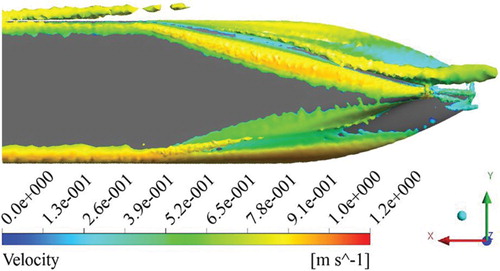
As the drift angle increases, the flow and vorticity distribution around the hull become more complicated. At 12° drift, the fore-body bilge vortex, fore-body side vortex, aft-body bilge vortex, and aft-body side vortex can be clearly observed in the figures. The fore-body bilge vortex, fore-body side vortex, aft-body bilge vortex, and aft-body side vortex extend to the windward side of the hull. The fore-body bilge vortex and fore-body side vortex extend farther along with the increase of drift angle. The aft-body vortices are combined into the aft-body side vortex and aft-body bilge vortex. The strength of the aft-body side vortex and aft-body bilge vortex enhance along with the increase of drift angle. Compared with the prediction under the RNG $k-\epsilon$ turbulence model, the fore-bilge vortex is more obvious in the SST $k-\omega$ case. The ship stern vorticity is shown in Figure 12.

Figure 12. Representation of the ship stern vorticity by means of the Q criteria at Q = 0.02, with the SST $k-\omega$ turbulence model ($\beta ={12}^{\circ }$).

4.5. Surface flow features

The flow-field topology on or very near the hull can be examined by deducing certain information about the complex 3D flow features. Surface features based on the topology can substantially affect the behaviour of the off-surface flow field. The skin friction defines a continuous vector field on the hull surface, and curves tangent to the skin friction vector are referred to as skin friction lines or limited streamlines. Figure 13 presents views of the mean and time-averaged limited streamlines from underneath the hull at various drift angle when using the SST $k-\omega$ turbulence model.

Figure 13. Bottom view of mean and time-averaged limited streamlines at different drift angle with the SST $k-\omega$ turbulence model.

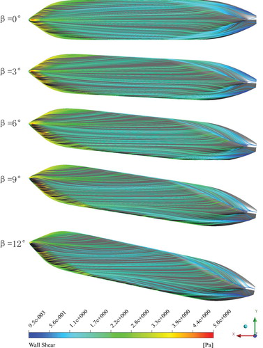
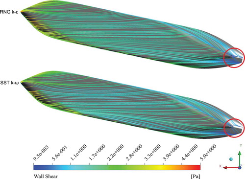
At 0° drift, the limited streamlines generally follow the hull curvature over the fore-body, run parallel to the mid-body section, and taper towards the stern. As the drift angle increases, the mean and time-averaged surface flows become considerably more complicated. At the same time, the surface flow spirals, initiating the aft-body side vortex. Note that the limited streamlines differ according to whether the RNG $k-\epsilon$ turbulence model or the SST $k-\omega$ turbulence model is used, as seen in Figure 14. Compared with the RNG $k-\epsilon$ turbulence model, the hook shape can be predicted well under the SST $k-\omega$ turbulence model and the limited streamlines become more complex at the stern.

Figure 14. Bottom view of mean and time-averaged limited streamlines at $\beta ={12}^{\circ }$ with the RNG $k-\epsilon$ turbulence model and SST $k-\omega$ turbulence model.

5. Calculation of maneuvering derivatives

Marine simulators play an important role in marine training projects. Figure 15 shows a marine simulator developed by our research group. The mathematical model of ship maneuvering motions is a key component in the marine simulator. The numerical results presented in this paper are used to improve the mathematical model of ship maneuvering motions in the marine simulator.

Figure 15. Marine simulator based on the numerical results presented in the previous section.

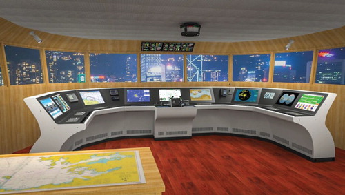
The numerical CFD results are used to derive the maneuvering derivatives, and these are compared with those given by MOERI experimental data. The maneuvering derivatives from the CFD data help to improve the accuracy of mathematical models of ship maneuvering motions, and enable the ship maneuvering motions to be predicted.

When the ship moves obliquely at a certain drift angle β, the velocity components u and v in the body-fixed coordinate system can be expressed as (11a) $\begin{array}{rl}u& =U\cos \beta \end{array}$(11a) (11b) $\begin{array}{rl}v& =-U\sin \beta \end{array}$(11b) The lateral force Y and moment N have been calculated at various drift angle in the numerical simulation. Thus, $Y-v$ and $N-v$ curves can be plotted. Considering the port-and-starboard symmetry, the mathematical model relating Y, N, and v can be expressed as (12a) $\begin{array}{rl}Y& =Y_0+Y_{v}v+\frac{1}{6}{Y}_{vvv}{v}^3\end{array}$(12a) (12b) $\begin{array}{rl}N& =N_0+N_{v}v+\frac{1}{2}{N}_{vvv}{v}^3\end{array}$(12b) Where $Y_v$, $Y_{vvv}$, $N_v$, $N_{vvv}$ are the maneuvering hydrodynamic derivatives, and $Y_0$, $N_0$ are the lateral force and moment, respectively, at the initial steady state of forward motion. Dividing Equation (12a) by $(1/2)\rho L^2{U}^2$ and dividing Equation (12b) by $(1/2)\rho L^3{U}^2$, where $\rho$ is the mass density of water, L is the ship length, and U is the ship speed. The dimensionless form of Equations (13a) and (13b) can be expressed as (13a) $\begin{array}{rl}{Y}^{\mathrm{\prime }}& =Y_0^{\mathrm{\prime }}+Y_v^{\mathrm{\prime }}{v}^{\mathrm{\prime }}+\frac{1}{6}{Y}_{vvv}^{\mathrm{\prime }}{v}^{\mathrm{\prime }3}\end{array}$(13a) (13b) $\begin{array}{rl}{N}^{\mathrm{\prime }}& =N^{\mathrm{\prime }}+N_v^{\mathrm{\prime }}{v}^{\mathrm{\prime }}+\frac{1}{2}{N}_{vvv}^{\mathrm{\prime }}{v}^{\mathrm{\prime }3}\end{array}$(13b) The dimensionless maneuvering derivatives can be obtained using regression formulae, and the regression curves are shown in Figures 16 and 17. The linear derivatives $Y_v^{\mathrm{\prime }}$, $N_v^{\mathrm{\prime }}$ derived from MOERI experimental data and CFD data are presented in Table 7. The results are in reasonably good agreement.

Figure 16. Regression curves of maneuvering derivative $Y_v^{\mathrm{\prime }}$.

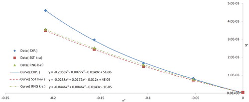
Figure 17. Regression curves of maneuvering derivative $N_v^{\mathrm{\prime }}$.

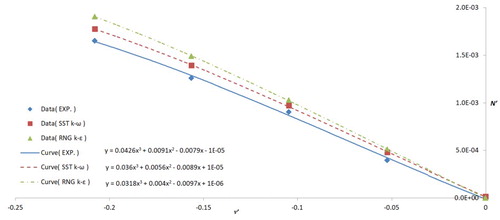
Table 7. Calculation of maneuvering derivatives.

Derivatives	$Y_v^{\mathrm{\prime }}$	$N_v^{\mathrm{\prime }}$
MOERI EXP.	−0.0149	−0.0079
CFD SST $k-\omega$	−0.0120	−0.0089
CFD RNG $k-\epsilon$	−0.0143	−0.0097

6. Conclusion

This paper investigates the flow around the KVLCC2 model at different drift angles using the RANS method in combination with the RNG $k-\epsilon$ and SST $k-\omega$ turbulence models. Three different mesh conditions are employed to perform the verification and validation based on the methodology and procedures suggested by ITTC. The absolute value of comparison error E for C_X, C_Y and C_N are 4.5%D, 10.3%D and 6.4%D respectively, which are smaller than the validation uncertainty U_V. The validation is successful at the present U_V level. The hydrodynamic forces and yaw moment acting on the KVLCC2 model are calculated under the different turbulence models and drift angles, and the numerical results are compared with experimental results. The deviation between numerical and experimental results begins to increase along with the increase of drift angle. Compared with the RNG $k-\epsilon$ turbulence model, the numerical results with SST $k-\omega$ turbulence model are closer to the experimental results.

The surface pressure distribution, vorticity distribution, and surface flow features around the hull are observed and analysed. By comparing the surface pressure distribution with experimental results, it is apparent that the SST $k-\omega$ turbulence model is closer to the experimental output. The simulation captures the basic flow structure which includes fore-body bilge vortex, fore-body side vortex, aft-body bilge vortex, and aft-body side vortex at different drift angle. The fore-body bilge vortex and fore-body side vortex extend farther along with the increase of drift angle. Compared with the prediction under the RNG $k-\epsilon$ turbulence model, the details of vortex is more obvious in the SST $k-\omega$ case.

At last, the maneuvering derivatives are calculated based on numerical results to create the mathematic model of ship maneuvering motions in the marine simulator and predict the ship maneuvering motions. This method will try to promote the practicality of CFD technology.

Disclosure statement

No potential conflict of interest was reported by the authors.

ORCID

Xiao Yang http://orcid.org/0000-0002-9573-8782

Yong Yin http://orcid.org/0000-0002-2947-5275

Additional information

Funding

The current work was supported by Natural Science Foundation of Liaoning Province [No. 20170540085 & No. 2019-ZD-0166]; and the Fundamental Research Funds for the Central Universities of China [No. 3132018306]; and the educational reform project of Dalian Maritime University [No. 2017Y05 & No. 2018Y09].

References

- Abbas N, Kornev N. 2016. Validation of hybrid URANS/LES methods for determination of forces and wake parameters of KVLCC2 tanker at manoeuvring conditions. Ship Technol Res. 63(2):96–109. doi: 10.1080/09377255.2016.1157275
- Degani D, Seginer A, Levy Y. 1990. Graphical visualization of vortical flows by means of helicity. AIAA J. 28(8):1347–1352. doi: 10.2514/3.25224
- Feng SB, Zou ZJ, Zou L. 2015. Numerical calculation of hydrodynamic forces on a KVLCC2 hull-rudder system in oblique motion. J Shanghai Jiaotong Univ. 49(4):470–474.
- Fureby C, Toxopeus SL, Johansson M, Tormalm M, Petterson K. 2016. A computational study of the flow around the KVLCC2 model hull at straight ahead conditions and at drift. Ocean Eng. 118:1–16. doi: 10.1016/j.oceaneng.2016.03.029
- He S, Kellett P, Yuan ZM, Incecik A, Turan O, Boulougouris E. 2016. Manoeuvring prediction based on CFD generated derivatives. J Hydrodyn Ser B. 28(2):284–292. doi: 10.1016/S1001-6058(16)60630-3
- Hunt JCR, Wray AA, Moin P. 1988. Eddies, stream, and convergence zones in turbulent flows. Center for Turbulence Research Report. CTR–S88.
- Jin YT, Duffy J, Chai SH, Chin C, Bose N. 2016. URANS study of scale effects on hydrodynamic manoeuvring coefficients of KVLCC2. Ocean Eng. 118:93–106. doi: 10.1016/j.oceaneng.2016.03.022
- Kamkar SJ, Jameson A, Wissink AM, Sankaran V. 2010. Feature-driven cartesian adaptive mesh refinement in the helios code. Paper presented at: 48th AIAA Aerospace Sciences Meeting Including the New Horizons Forum and Aerospace Exposition. p. 2010–2171.
- Kume K, Hasegawa J, Tsukada Y, Fujisawa J, Fukasawa R, Hinatsu M. 2006. Measurements of hydrodynamic forces, surface pressure, and wake for obliquely towed tanker model and uncertainty analysis for CFD validation. J Mar Sci Technol. 11(2):65–75. doi: 10.1007/s00773-005-0209-y
- Meng Q-J, Wan D-C. 2016. Numerical simulations of viscous flow around the obliquely towed KVLCC2M model in deep and shallow water. J Hydrodyn Ser B. 28(3):506–518. doi: 10.1016/S1001-6058(16)60655-8
- Menter FR. 1994. Two-equation eddy-viscosity turbulence models for engineering applications. AIAA J. 32(8):1598–1605. doi: 10.2514/3.12149
- Park D-M, Lee J, Kim Y. 2015. Uncertainty analysis for added resistance experiment of KVLCC2 ship. Ocean Eng. 95:143–156. doi: 10.1016/j.oceaneng.2014.12.007
- Pereira FS, Eça L, Vaz G. 2017. Verification and validation exercises for the flow around the KVLCC2 tanker at model and full-scale Reynolds numbers. Ocean Eng. 129:133–148. doi: 10.1016/j.oceaneng.2016.11.005
- Sadat-Hosseini H, Wu P-C, Carrica PM, Kim H, Toda Y, Stern F. 2013. CFD verification and validation of added resistance and motions of KVLCC2 with fixed and free surge in short and long head waves. Ocean Eng. 59:240–273. doi: 10.1016/j.oceaneng.2012.12.016
- Stern F, Wang ZY, Yang JM, Sadat-Hosseini H, Mousaviraad M, Bhushan S, Diez M, Sung-Hwan Y, Wu P-C, Yeon SM, et al. 2015. Recent progress in cfd for naval architecture and ocean engineering. J Hydrodyn Ser B. 27(1):1–23. doi: 10.1016/S1001-6058(15)60452-8
- Tian XM, Zou ZJ, Wang HM. 2010. Computation of the viscous flow and hydrodynamic forces on a KVLCC2 model in oblique motion. J Ship Mech. 14(8):834–840.
- Toxopeus SL, Simonsen CD, Guilmineau E, Visonneau M, Xing T, Stern F. 2013. Investigation of water depth and basin wall effects on KVLCC2 in manoeuvring motion using viscous-flow calculations. J Mar Sci Technol. 18(4):471–496. doi: 10.1007/s00773-013-0221-6
- Turnock SR, Phillips AB, Furlong M. 2008. URANS simulations of static drift and dynamic manoeuvres of the KVLCC2 tanker. Paper presented at: Proceedings of the workshop on verification and validation of ship manoeuvring simulation methods (SIMMAN 2008). p. 13–17.
- Van Hoydonck W, Toxopeuse S, Eloot K, Bhawsinka K, Queutey P, Visonneau M. 2019. Bank effects for KVLCC2. J Mar Sci Technol. 24(1):174–199. doi: 10.1007/s00773-018-0545-3
- Wang XQ, Liu HX, Ma S, Guo C. 2017. Investigation of the hydrodynamic model test of forced rolling for a barge using PIV. Chin J Ship Res. 12(2):49–56.
- Wang H-M, Zou Z-J, Tian X-M. 2009. Computation of the viscous hydrodynamic forces on a KVLCC2 model moving obliquely in shallow water. J Shanghai Jiaotong Univ. 14(2):241–244. doi: 10.1007/s12204-009-0241-x
- Wu XH, Liu ZY, Shi SD, et al. 2005. Ship maneuverability. Beijing: National Defence Industry press.
- Xing T, Bhushan S, Stern F. 2012. Vortical and turbulent structures for KVLCC2 at drift angle 0, 12, and 30 degrees. Ocean Eng. 55:23–43. doi: 10.1016/j.oceaneng.2012.07.026
- Yakhot V, Orzag SA. 1986. Renormalization group analysis of turbulence. I. Basic theory. J Sci Comput. 1(1):3–51. doi: 10.1007/BF01061452
- Yang X, Yin Y, Lian JJ. 2019. Numerical study on the hydrodynamic performance of the semi-spade rudder and propeller. Adv. Mech. Eng. 11(1):1–18.
- Yasukawa H, Yoshimura Y. 2015. Introduction of MMG standard method for ship maneuvering predictions. J Mar Sci Technol. 20(1):37–52. doi: 10.1007/s00773-014-0293-y